CONSTRAINING H₀ FROM CHANDRA OBSERVATIONS OF Q0957+561

Abstract

We report the detection of the lens cluster of the gravitational lens (GL) system Q0957+561 from a deep observation with the Advanced CCD Imaging Spectrometer on-board the Chandra X-ray Observatory. Intracluster X-ray emission is found to be centered 4${}^{\prime\prime}\!\!.$3${}_{-1.3}^{+1.3}$ east and 3${}^{\prime\prime}\!\!.$5${}_{-0.6}^{+1.2}$ north of image B, nearer than previous estimates. Its spectrum can be modeled well with a thermal plasma model consistent with the emission originating from a cluster at a redshift of 0.36. Our best-fit estimates of the cluster temperature of T_e = 2.09${}_{-0.54}^{+0.83}$ keV (90% confidence) and mass distribution of the cluster are used to derive the convergence parameter $\kappa$, the ratio of the cluster surface mass density to the critical density required for lensing. We estimate the convergence parameter at the location of the lensed images A and B to be ${\kappa_{A}}$ = 0.22${}^{+0.14}_{-0.07}$ and ${\kappa_{B}}$ = 0.21${}^{+0.12}_{-0.07}$, respectively (90% confidence levels). The observed cluster center, mass distribution and convergence parameter $\kappa$ provide additional constraints to lens models of this system. Our new results break a mass-sheet degeneracy in GL models of this system and provide better constraints of $\sim$ 29% (90% confidence levels) on the Hubble constant. We also present results from the detection of the most distant X-ray jet (z = 1.41) detected to date. The jet extends approximately 8″ NE of image A and three knots are resolved along the X-ray jet with flux densities decreasing with distance from the core. The observed radio and optical flux densities of the knots are fitted well with a synchrotron model and the X-ray emission is modeled well with inverse Compton scattering of Cosmic Microwave Background photons by synchrotron-emitting electrons in the jet.

1. INTRODUCTION

In an earlier paper based on deep ROSAT observations, we had reported the 3 $\sigma$ detection of X-rays from the cluster of galaxies of the gravitational lens system Q0957+561 (Chartas et al. 1998). This cluster contributes to the lensing of a distant z = 1.41 radio loud quasar. The lensed quasar appears as two images separated by 6${}^{\prime\prime}\!\!.$17 and denoted as A (north) and B (south). An accurate determination of the mass distribution of the cluster is essential in reducing the uncertainty of the Hubble constant as derived from the application of Refsdal’s lensing method (Refsdal, 1964a,1964b). Due to the limited spatial and spectral resolution and low signal-to-noise ratio of the previous X-ray observations, only weak constraints could be placed on the cluster properties. In particular, we obtained estimates for the convergence parameter, $\kappa$, the ratio of the projected two-dimensional (2D) surface mass density of the cluster to the critical surface mass density of the lens cluster. We found $\kappa$ to range between 0.07 and 0.21, when assuming that the cluster center was located 24″ away from image B, a separation based on optical observations of the galaxy members of the cluster (Angonin-Willaime et al. 1994). Other methods for estimating the convergence parameter $\kappa$ rely on weak-lensing of background galaxies (Fischer et al. 1997), measurements of the velocity dispersion of the lens galaxy G1 (Falco et al., 1997; Tonry & Franx 1999; Romanowsky & Kochanek 1999) and measurements of the velocity dispersion of the lens cluster (Garrett, Walsh, & Carswell 1992, Angonin-Willaime, Soucail, & Vanderriest 1994). The present constraints on $\kappa$ are quite poor and have probably underestimated the systematic errors due to the uncertainty of the location of the cluster center and of the mass profile. Barkana et al. (1999) found a strong dependence of $\kappa$ on the assumed cluster mass profile and on the distance of the cluster center from the lens galaxy.

A measurement of the convergence parameter $\kappa$ at the location of the lensed images with respect to the cluster center is needed to break the Hubble constant mass-sheet degeneracy (Falco et al. 1985). More direct methods of determining the location of the center of mass of the cluster are provided by measurements of the intracluster medium emission in the X-ray band, the weak lensing method, and optical measurements of the member galaxies. X-ray measurements with ROSAT did not provide any useful constraints on the location of the cluster center. The weak lensing method, which determines the mass distribution of the lens cluster from the gravitational distortion of the images of background galaxies, yields a center of mass of the cluster to be located $\sim$ 18″ east and 13″ north of G1, with a 1$\sigma$ uncertainty of about 15″. Angonin-Willaime et al. (1994) derived a center for the cluster at 13${}^{\prime\prime}\!\!.$7 west, 19${}^{\prime\prime}\!\!.$6 south of image B by proportionally weighting galaxies by their R band luminosity. This method was found to be very sensitive to the number of galaxies included in the calculation. For example, Garrett et al. (1992) using a subset of the galaxies had found the cluster center at 3${}^{\prime\prime}\!\!.$5 west and 1${}^{\prime\prime}\!\!.$2 north of G1. Another method for estimating the cluster center is based on the “best-fit” values for the lens models that describe this system. In a recent analysis Chae et al. (1999) model the cluster contribution by a power-law sphere with an extended core. They found a distance between the cluster center and the G1 galaxy of 9^′′${}_{-4}^{+4}$ and a position angle $\theta$ (North through East) of $\sim$ 52^∘. In an independent analysis Barkana et al. (1999) model the cluster as a singular isothermal sphere and allow the center position and velocity dispersion of the cluster to be free parameters. They found a value for the distance of the cluster center from the G1 galaxy of 13${}^{\prime\prime}\!\!.$7 east, 6${}^{\prime\prime}\!\!.$9 north and a value for the velocity dispersion of 439 km s^-1. The large systematic differences between independent estimates of the center position of the cluster obtained through modeling imply that the mass distribution of the lens is not accounted for correctly in these models. A recent discovery of the lensed images of the host galaxy of the quasar Q0957+561 by Keeton et al. (2000) has provided tighter constraints on the global structure of the lensing potential. Gravitational-lens (GL) models of Q0957+561 developed prior to the discovery of the host galaxy failed to reproduce the correct shape for the host galaxy arcs and therefore any constraints they provide on the value of the center location of the cluster are unreliable. Lens models by Keeton et al. (2000) that incorporate the constraints provided by the host galaxy arcs imply that the cluster potential is approximately centered on G1.

In this paper we present results from the recent observation of the GL system Q0957+561 with the Chandra X-ray Observatory. Section 2 contains a description of the observation and the data reduction. In section 3 we perform a detailed spatial analysis of the X-ray image of the lens cluster and present a more direct measurement of the location of the cluster center and the cluster core radius. In section 3 we also briefly describe the detection of an X-ray jet corresponding to the radio jet from image A. The spectral analyses of the lens cluster, lensed images, and X-ray jet are presented in section 4. We revisit the determination of the convergence parameter, $\kappa$, in section 5. In section 6 we discuss the implications of the Chandra constraints on the Hubble constant and conclude with a summary of the results obtained from the Chandra observation. We use $H_{0}$ = 75 km s^-1 Mpc^-1, $q_{0}$ = 0.5, and $\Lambda$ = 0, unless mentioned otherwise. At the redshifts of 0.36(lens) and 1.41(quasar) an angular size of 1″ corresponds to length scales of $\sim$ 4.1 kpc and $\sim$ 5.7 kpc, respectively.

2. OBSERVATIONS AND ANALYSIS

Q0957+561 was observed with the ACIS instrument (Garmire et al. 2001, in preparation) onboard the Chandra X-ray Observatory in 2000 April 4 for 47,660s. The data were collected on the back-illuminated S3 CCD of ACIS. The instrument was operated in sub-array mode where a restricted region with 254 of 1024 rows of the chip collects data to reduce the frame-time from the nominal 3.24 s(full-frame) to 0.741 s. The telescope pointing was set approximately 1 arcmin off axis. We used the sub-array mode and off-axis pointing to reduce the probability of multiple X-rays landing within a few CCD pixels during the same CCD frame readout. This effect, commonly referred to as pile-up, may lead to spectral and spatial distortions and loss of detected events. The detected count rates for images A and B are 0.21 counts s^-1 and 0.16 counts s^-1, with respective estimated pile-up fractions of about 11% and 7% for the 0.741 s frame-time. We applied the data processing techniques recommended by the Chandra X-ray Center (CXC) which include removal of hot pixels and non-X-ray events. The standard CXC software pipelines randomize the event positions by $\pm$ 0${}^{\prime\prime}\!\!.$246 (1 ACIS pixel = 0${}^{\prime\prime}\!\!.$492), in each spatial coordinate. This randomization is done to avoid aliasing effects noticeable in observations with exposure times less than $\sim$ 2 ks. Since the exposure time for the Chandra observation of Q0957+561 is considerably longer than 2 ks, we reprocessed the data with the CXC software tool ACISPROCESSEVENTS without randomizing the event positions. This reprocessing led to an improvement of the 50 percent encircled energy radius from 0${}^{\prime\prime}\!\!.$40 to 0${}^{\prime\prime}\!\!.$35. The CCD read-out streaks of the bright images A and B of Q0957+561 are removed in the spatial and spectral analysis. These streaks are produced from events that are recorded on the CCD during the transfer of charge into the CCD frame-store region. The background level was fairly constant throughout the observation with a mean value of 2.2 $\times$ 10^-6 events s^-1 arcsec^-2 in the 0.3-7 keV band.

3. SPATIAL ANALYSIS; NEW X-RAY COMPONENTS IDENTIFIED

3.1. The Lens Cluster

In Figure 1 we show the Chandra image of the GL system Q0957+561. To enhance the presence of soft extended X-ray emission, the image was filtered to include only photons with energies ranging between 0.5 and 3.0 keV. This choice of energy range is supported by the analysis of the extracted spectrum of the cluster (see section 4.1) which indicates that the cluster spectrum is very soft with most of the detected counts lying below 3 keV. The image has been binned with a bin size of 0${}^{\prime\prime}\!\!.$5 and smoothed with the software tool CSMOOTH developed by Ebeling et al. (2000) and provided by the Chandra X-ray Center (CXC). CSMOOTH smoothes a two-dimensional image with a circular Gaussian kernel of varying radius. Extended X-ray emission with a radius of $\sim$ 30″, encompassing the quasar images, is clearly visible in Figure 1. The extended emission appears to be centered slightly northeast of image B. This is seen if one takes the midpoint of the two outer contour levels of the X-ray emission shown in Figure 1. The midpoint is slightly to the east of image B.

To constrain the morphology of the soft extended emission we performed a 2D fit to the X-ray data using the model described below. The spatial model has the following three components: extended cluster emission, unresolved emission from the quasar images and background emission.

(a) To describe the cluster brightness profile, we use a $\beta$ model

$${\centering f(r)=A[1+(\frac{r}{r_{c}})^{2}]^{-3{\beta}+\frac{1}{2}}\@add@centering}$$ (1)

where,

$$r(x,y)~{} = ~{}\frac{\sqrt{{x^{\prime}}^{2}(1-{\epsilon})^{2}+{y^{\prime}}^{2}}}{1-{\epsilon}}$$

$$x^{\prime}~{} = ~{}(x-x_{\rm 0})\cos({\theta})+(y-y_{\rm 0})\sin({\theta})$$

$$y^{\prime}~{} = ~{}(y-y_{\rm 0})\cos({\theta})-(x-x_{\rm 0})\sin({\theta})\,,$$

$\epsilon$ is the ellipticity of the model defined here as $\epsilon=1-q$; $q$ is the axis ratio; $\theta$ is defined as the angle between the major axis and west, and is measured west to north; $x_{\rm 0},y_{\rm 0}$ are the positions of the cluster center; and $\beta$ is the ratio of kinetic energy per unit mass in galaxies to kinetic energy per unit mass in gas.

(b) To model the lensed quasar images, we use simulated point spread functions (PSF’s). The centroids of the model PSF’s are fixed to the observed image centroids. The relative normalization of the PSFs is the flux ratio of the lensed images as determined from annular regions of inner and outer radii of 0${}^{\prime\prime}\!\!.$5 and 2″, respectively, centered on the images. These annuli were chosen to avoid the slightly piled-up cores of the images. The model PSFs appropriate for this observation were created employing the simulation tool MARX v3 (Wise et al. 1997) with an input spectrum derived from the best-fit Chandra spectrum of the lensed images. Specifically, we used an absorbed power law with a column density of N_H = 0.82 $\times$ 10²⁰ cm^-2 (Dickey & Lockman, 1990) and photon indices of $\Gamma$ = 2.08 and 1.94 for images A and B respectively (see section 4.2). Here-after the term best-fit is used to describe a result obtained by fitting a model to our data using an optimization technique to find the local fit-statistic minimum. The Levenberg-Marquardt optimization method is used for the spectral analysis, the Powell method is used for the spatial analysis of the cluster and the downhill simplex method is used by the fitting tool LYNX (section 4.2).

(c) Finally in our model, we include a uniform background of 0.01 events per pixel obtained from a background region at the same distance from the aim point as the cluster.

In determining the cluster properties, we omitted a 10″ radius region centered on the midpoint between the quasar images to avoid biasing the fit due to residuals in modeling the cores of the PSFs. For the annulus from 8″ to 40″ centered on the midpoint of the quasar images, we binned the image in 1″ pixels and smoothed this with a Gaussian ($\sigma=3{\arcsec}$) prior to performing the spatial fitting. The fits were performed with the CXC software package SHERPA. To evaluate the sensitivity of the results to the choice of assumptions made for sizes of spatial windows and bin sizes of the data, we performed the spatial analysis over a wide range of input model parameters. Specifically, we binned the X-ray data with bin sizes varying between 1″ and 2″. The annulus region used to model the cluster was varied with an inner radius ranging between 10″ and 14″ and an outer radius ranging between 30″ and 40″. The errors quoted for the spatial model parameters represent the maximum uncertainties obtained from all spatial fits. Results for our spatial fits are presented in Table 1. We find the center of the mass of the lens cluster to be located at ${\Delta}{\alpha}$ = 4${}^{\prime\prime}\!\!.$3${}_{-1.3}^{+1.3}$ east, ${\Delta}{\delta}$ = 3${}^{\prime\prime}\!\!.$5${}_{-0.6}^{+1.2}$ north of the core of image B. The fits indicate that the smoothed mass distribution of the cluster is close to spherical with an ellipticity ${\epsilon}=0.19_{-0.08}^{+0.06}$. The best-fit values for $\beta$ and the core radius of the cluster are $\beta$ = 0.47${}_{-0.06}^{+0.06}$ and r₀ = 15${}^{\prime\prime}\!\!.$4${}_{-3.5}^{+3.5}$ (62.5 kpc), respectively. Our values for $\beta$ and $r_{0}$, within the uncertainties, fall on the trend line of $\beta$ versus $r_{0}$ obtained previously for a suite of galaxy clusters (Jones & Forman 1999).

3.2. The X-ray Jet of Image A

We notice a faint feature in the Chandra image extending northeast of image A that is aligned with the radio jet and appears to have a jet-like morphology. The X-ray jet is significant at the 4 $\sigma$ level. At a redshift of 1.41 this is the most distant X-ray jet detected to date. An overlay between this X-ray jet feature and a 3.6 cm radio map of the jet in image A (radio data from Harvanek et al. 1997) is shown in Figure 2. The X-ray and radio jet morphologies appear to be somewhat similar. A comparison between the radio and X-ray jet profiles along the jet ridge line is shown in Figure 3. The X-ray jet extends NE about 8″ from the core of image A with bright knots at 2${}^{\prime\prime}\!\!.$3, 4″ and 6″ (here-after also referred to as knots A, B and C, respectively) from the core. Each of these knots coincides within 0${}^{\prime\prime}\!\!.$5 with radio knots at similar locations. The intensity of the X-ray knots appears to decay as a function of distance from the core in contrast to the radio knots which become brighter at larger distances from the core. One possible interpretation of the former is that the jet flow is decelerating and the brightness change is due to aging of the higher energy electron population of the jet. The increase in the radio brightness along the jet may be due to an increase of the magnetic field strength. A similar anti-correlation between radio and X-ray profiles was recently reported in 3C273 (Sambruna et al. 2001; Marshall et al. 2001). Lens models for Q0957+561 predict a small magnification gradient along the jet. We estimate that the magnifications for the knots B and C are 1.9 and 1.6, respectively. Therefore, the magnification gradient does not greatly change the X-ray and radio brightness profiles. In section 4.3 we briefly discuss possible mechanisms that may explain the origin of the X-ray jet emission and present the spectral energy distribution for knots B and C.

4. SPECTRAL ANALYSIS

4.1. A Cool Lens Cluster

The spectrum for the cluster of galaxies was extracted from a 40″-radius circle centered on the X-ray determined cluster center. Beyond this radius, cluster emission is not detected above the background. Three-arcsecond-radius circles centered on images A and B were excluded. Emission from the X-ray jet was also excluded by omitting a rectangle 2${}^{\prime\prime}\!\!.$5 by 7″. However, even beyond the 3″ radius, mirror scattering of the bright lensed images produces a significant contamination of the cluster spectrum, particularly at hard energies. We estimate the spectrum of the contamination produced by images A and B to the cluster spectrum by performing simulations with the raytrace simulator tool MARX provided by the CXC. We simulate two point sources centered at the locations of images A and B with input spectra and normalizations derived from our spectral analysis of these images. We find a total of about $\sim$ 200 counts due to quasar emission ($\sim$ 0.8% of the total counts from images A and B) within the cluster extraction region. The CCD background and quasar contamination are subtracted from the cluster region resulting in the spectrum shown in Figure 4. A net total of about $\sim$ 600 X-ray events originate from the cluster. The data were fit with the spectral analysis tool XSPEC (Arnaud 1996). We model the cluster spectrum with a Raymond - Smith thermal plasma modified by absorption due to our Galaxy. The Galactic column density is fixed at the value of N_H = 0.82 $\times$ 10²⁰ cm^-2 for all spectral fits performed in our analysis. We assumed a typical value for the metal abundances in clusters of 30% solar (see, e.g., Henriksen 1985; Hughes et al. 1988; and Arnaud et al. 1987). Due to the relatively low signal-to-noise ratio of the cluster spectrum the metal abundances of the cluster cannot be constrained within useful limits. If we let the abundance be a free parameter we obtain a best-fit value for the abundance of A = 0.19${}_{-0.19}^{+0.54}$ (90% confidence level) and a best fit temperature of 2.1keV. We note that the choice of metal abundance (between 0 and 100% solar) has little effect on the temperature determinations. The abundance ratios used in the Raymond - Smith thermal plasma emission model are those of Anders & Grevesse (1989). Our best-fit model is shown in Figure 4. The uncertainty in the calibration of ACIS S3 below 0.5 keV contributes to the large residuals between 0.4 and 0.5 keV. We find a temperature for the cluster of T_e = 2.09${}_{-0.54}^{+0.83}$ keV at the 90% confidence level. The spectral line features between 0.7 and 0.9 keV (observed frame) correspond to a redshifted z= 0.36 complex of Fe L lines. Our spectral analysis thus confirms that the extended emission originates from the lens. The relatively low cluster temperature of $\sim$ 2 keV and our values of $\beta$ and the core radius from section 3.1, within their uncertainties, are consistent with the observed correlations between temperature, $\beta$ and core radius obtained previously for a large sample of clusters of galaxies (Jones & Forman 1999). We estimate that $\sim$ 3% of the counts originating from cluster emission are excluded from our extracted spectrum due to the regions used in our analysis. Correcting for this effect we find a 2 - 10 keV cluster luminosity of 4.7 $\times$ 10⁴² erg s^-1. Our estimated values for L_X and T_e are consistent with the empirical L_X - T_e correlation between cluster luminosity and temperature of, $T_{keV}$ = 0.13(+0.08,-0.07) $\times$ $L_{40}^{(0.351\pm 0.068)}$, where $L_{40}$ is the measured 0.5-4.5 keV luminosity in units of 10⁴⁰ erg s^-1 ($H_{0}$ = 50 km s^-1 Mpc^-1) (Jones & Forman 1999; Markevitch, 1998). Specifically, the L_X - T_e correlation yields a value of T_e $\sim$ 2 keV for our value of $L_{40}$ = 2.3 $\times$ 10³.

4.2. The Spectra of Images A and B

As mentioned in section 2, we expect the spectra of images A and B to be slightly piled-up. We used two independent methods to account for pile-up.

In the first method we extracted spectra from annuli centered on each image with inner and outer radii of 0${}^{\prime\prime}\!\!.$5 and 3″, respectively. Pile-up is significantly reduced beyond the 0${}^{\prime\prime}\!\!.$5 radius, in the wings of the PSFs. One of the drawbacks of the annulus method is that only $\sim$ 40% of the total quasar counts are considered in the spectral fit, thus, leading to larger uncertainties in the values of the estimated parameters. We corrected the ancillary files provided by the CXC to account for the energy dependence of X-ray scattering in the Chandra mirrors within the selected annuli. The energy dependent correction function was evaluated by performing raytrace simulations with the software tool MARX. We modeled the spectra with power-laws modified by absorption from our Galaxy. The fits are statistically acceptable ($\chi^{2}(\nu)=113(138)$ and $\chi^{2}(\nu)=109(105)$, for images A and B, where $\nu$ is the number of degrees of freedom) with best-fit values for the photon indices of images A and B of 2.06${}^{+0.04}_{-0.05}$ and 2.06${}^{+0.05}_{-0.05}$, respectively (90% confidence errors). The flux ratio B/A is 0.74 $\pm$ 0.02, consistent with the observed flux ratio in the radio band of 0.76 $\pm$ 0.03 (VLBI $\lambda$ 13cm, Falco et al. 1991) and 0.72 $\pm$ 0.04 (VLA $\lambda$ 6cm core, Conner et al. 1992). Previous measurements of the X-ray flux ratios of 0.3 $\pm$ 0.1 and 1.5 $\pm$ 0.2 made with EINSTEIN and ROSAT, respectively,(Chartas et al. 1998) differed significantly from this value, suggesting the presence of microlensing for those epochs.

For our second approach we used the forward fitting tool LYNX developed at PSU (Chartas et al. 2000). Spectra were extracted from circles centered on each image with radii of 3″. We found the photon indices for A and B to be 2.08 $\pm$ 0.03 and 1.94 $\pm$ 0.03 (90% confidence errors). The 0.5-10 keV X-ray fluxes of images A and B corrected for pile-up are 11.6 $\pm$ 0.9 $\times$ 10^-13 erg s^-1 cm^-2 and 8.8 $\pm$ 0.7 $\times$ 10^-13 erg s^-1 cm^-2. The errors in the estimates of the photon indices in both methods do not include systematic errors due to the uncertainties in the ACIS detector quantum efficiency and energy responce. We note that the “annulus” method uses detector response matrices provided by the CXC whereas LYNX links to a Monte Carlo simulator of ACIS developed by the ACIS instrument team (Townsley et al., in preparation). We do not detect any line features in their spectra. Combining the spectra of images A and B, we place a 95% confidence upper limit of $\sim$ 60 eV (observed-frame) on the equivalent width of an intrinsically narrow fluorescent Fe K${\alpha}$ line at 6.4 keV (2.66 keV observed-frame).

4.3. The Spectral Energy Distribution of the Jet

In Figure 5 we show the spectral energy distribution(SED) of the two brightest knots B and C of the jet. The radio flux density, $F_{\nu}$, at 3.6 cm for jet A was based on the value reported by Harvanek et al. (1997). The jet knots have not been detected in the optical band; we therefore placed upper limits on the optical flux density of the knots based on deep HST observations of this field performed by Bernstein & Fischer (1997). We find the 3$\sigma$ upper limit on ${\nu}F_{\nu}$ at 5500 Å to be 5.6 $\times$ 10^-16 erg s^-1 cm^-2. The X-ray spectrum was extracted from a 2.5″ by 7″ rectangle. The background was extracted from several similar rectangles located at the same distance from image A but at different azimuths. A net total of 50 $\pm$ 8 X-ray events were those ascribed to the jet. We modeled the spectrum with a power-law modified by absorption due to our Galaxy. We find a best-fit value for the photon index $\Gamma$ of 1.87 $\pm$ 0.6 (90% confidence errors) including systematic errors estimated from using different background regions. We find ${\nu}F_{\nu}$ at 1 keV for knots B and C of 8.9 $\pm$ 2.8 $\times$ 10^-16 and 2.7 $\pm$ 0.9 $\times$ 10^-16 erg s^-1 cm^-2, respectively (90% confidence errors). A simple synchrotron model with a single power law distribution is not consistent with the SED of the jet in Q0957A. Given the high redshift of the jet, the energy density of the Cosmic Microwave Background (CMB) is enhanced by a factor of $(1+z)^{4}=33.7$ over the local value. We therefore modeled the spectra of knots B and C with a CMB model, in which cosmic microwave photons are inverse Compton scattered by synchrotron-emitting electrons in the jet. The solid and dashed lines in Figure 5 are the fits of the CMB model to the SEDs of knots B and C, respectively. We are able to fit both knots well with very moderate Doppler beaming (see Figure 5). We conclude that a plausible mechanism to explain the X-ray emission is inverse Compton scattering of CMB photons. Such a mechanism was shown to be consistent with the peculiar SED of the jet in PKS 0637-752 (Tavecchio et al, 2000).

5. MASS DISTRIBUTION AND CONVERGENCE OF THE LENS CLUSTER

For isothermal and spherical clusters of galaxies the equation for hydrostatic equilibrium can be solved for the virial mass, $M_{grav}(<r)$, within a radius $r$,

$${M_{grav}(<r)}=-{{{kTr}\over{\mu m_{p}G}}{{d~{}ln~{}\rho}\over{d~{}ln~{}r}}}$$ (2)

where $k$ is Boltzmann’s constant, $\mu$$m_{p}$ is the mean molecular weight of the cluster gas, and $\rho(r)$ is the cluster gas density at $r$.

Assuming a $\beta$ model for the density profile of the hot gas (e.g., Jones & Forman 1984) we obtain the equation for the total mass of the lens within a radius $r$,

$${M_{grav}(<r)}={{{3\beta kT}\over{\mu m_{p}G}}{{r}\over{[1+({{r_{c}}\over{r}})^{2}]}}}{\ ,}$$ (3)

By incorporating the best-fit spatial and spectral parameters from our present analysis (see Tables 1 and 2) we find the total cluster mass within a radius of 1 $h_{75}$^-1 Mpc to be M_grav = 9.9${}_{-3.8}^{+1.9}$ $\times$ 10¹³ M_⊙. In Figure 6 we show the total cluster mass within a radius $r$ as a function of radius. The shaded region indicates the allowed values for the cluster mass including the uncertainities obtained from the spatial and spectral fits to the lens cluster (see Tables 1 and 2).

These mass estimates were used to evaluate the convergence parameter ${\kappa}(x)$,

$${\kappa(x)={{\Sigma(x)}\over{\Sigma_{cr}}}}\,$$

where ${\Sigma(x)}$ is the surface mass density of the lens cluster as a function of the cylindrical radius $x$ (Chartas et al. 1998) and $\Sigma_{cr}$ is the critical surface mass density (see, e.g., Schneider, Ehlers & Falco 1992), In Figure 7 we plot the convergence parameter $\kappa(x)$ as a function of distance from the cluster center. The thick solid line corresponds to the best-fit spatial and spectral parameters. The largest contributor to the uncertainty in our estimate of $\kappa(x)$ is the weak constraint on the temperature of the cluster. To illustrate this we have plotted the uncertainty in $\kappa(x)$ assuming 68% (dotted lines) and 90% (dashed lines) confidence intervals for the temperature. We also chose cluster limits ranging from 0.7$r_{500}$ and 1.4$r_{500}$, where $r_{500}$ is the radius in which the mean over-density is 500, and $r_{500}$ = 1.58(T_X/10 keV)^1/2 $h^{-1}_{75}$ Mpc $\sim$ 0.71 $h^{-1}_{75}$ Mpc (Mohr, Mathiesen, & Evrard, 1999). The uncertainity in $\kappa$ introduced by assuming the cluster limit to range between 0.7 and 1.4$r_{500}$ is only $\sim$ 2%. Our assumption of spherical symmetry of the mass distribution has little effect on the estimate of the convergence parameter. Calculations of the mass distribution of the nonsperical cluster of galaxies A2256 (axis ratio $\sim$ 1.6) by Fabricant et al. (1984) showed that radially integrated mass estimates were negligibly affected by including an oblate or prolate cluster geometry. At the best-fit location of images A and B with respect to the cluster center, we estimate the convergences assuming the 90% confidence range in cluster temperature and find ${\kappa_{A}}$ = 0.22${}^{+0.14}_{-0.07}$ and ${\kappa_{B}}$ = 0.21${}^{+0.12}_{-0.07}$, respectively. Our estimated range of uncertainty in $\kappa$ does not include possible systematic errors arising from the estimation of the the surface mass density of the galaxy cluster through the use of a hydrostatic, isothermal $\beta$ model. Evrard, Metzler & Navarro (1999) have performed simulations to investigate the accuracy of galaxy cluster mass estimates based on X-ray observations. They found that estimates based on the hydrostatic, isothermal $\beta$ model are unbiased estimates of the mass of relaxed clusters with standard deviations of less than 30%. Recent observations of clusters of galaxies with XMM-Newton indicate that the cluster temperature profiles are remarkably isothermal beyond the central cooling flow (e.g., Arnaud et al. 2001). We therefore expect that our estimated uncertainity in $\kappa$ is dominated by the large uncertainity in the estimated value of the cluster temperature and not systematic errors introduced from the use of the isothermal $\beta$ model.

6. DISCUSSION AND CONCLUDIONS

Detailed lens models of Q0957+561 include the cluster’s contribution to the lensing potential by expanding the potential of the cluster in a Taylor series and keeping terms of up to third order (Kochanek 1991, Bernstein & Fischer 1999, Keeton et al. 2000). The second order term of the expansion represents the shear from the cluster and can be expressed as ${\gamma}={{\kappa}\over{({1+{\beta_{rd}}^{2}})^{3/2}}}$ where, ${\beta_{rd}}=r_{c}/d_{c}$, $r_{c}$ is the cluster core radius and $d_{c}$ is the distance from the cluster to the galaxy G1 (see, Kochanek, 1991). Recent models of Q0957+561 that incorporate additional constraints from observed arcs produced by the lensing of the quasar host galaxy imply a cluster shear amplitude, $\gamma$, that is relatively small compared to the convergence parameter $\kappa$ (Keeton et al. 2000). Other observations of Q0957+561 also favor values of $\kappa$ $>>$ $\gamma$ (Fischer et al. 1997; Romanowsky & Kochanek 1999; Chartas et al. 1998). As pointed out by Keeton et al. (2000), one way of producing $\gamma$ $<<$ $\kappa$ is to have the distance from the center of the cluster to the center of the lens galaxy be: less than the core radius for a cluster with a singular isothermal ellipsoid potential, or: less than the “universal” scale length for a cluster potential that follows the dark matter profile of Navarro, Frenk, and White (1996). Measurements at that time, ie., the late 1990s, indicated that the cluster center was located several core radii away from the lens (Fischer et al. 1997; Angonin-Willaime et al. 1994) and therefore were not consistent with the large value of $\kappa$ relative to the amplitude of the shear.

The Chandra observation of the cluster resolves this apparent discrepancy. We find the distance between the center of mass of the cluster and the center of the lens galaxy G1 to be $d_{c}$ = 4${}^{\prime\prime}\!\!.$8 considerably smaller than suggested from previous estimates. The best-fit position angle (North through East) and core radius of the cluster are $\sim$ 59^∘ and 15${}^{\prime\prime}\!\!.$4${}^{+3.5}_{-3.5}$, respectively. The Chandra observations of Q0957+561 therefore indicate that the cluster center is located within a core radius of the lens galaxy G1. Using the values for $r_{c}$, $d_{c}$, and ${\kappa}$ provided by our analysis of the Chandra observation of Q0957+561 we find that the cluster shear amplitude is $\gamma$ = 0.01 $\pm$ 0.009 (90% confidence level), consistent with the recent model results of Keeton et al. (2000). The Chandra observation of Q0957+561 has eliminated several uncertainties introduced in our previous analysis of the ROSAT HRI data of this system. Specifically, the temperature, the core radius, and cluster shape are now determined more reliably. Previous estimates of $\kappa$ are unreliable due to the large distances between the center of the cluster and the galaxy G1 assumed in these analyses. To evaluate the implication of our estimate of $\kappa$ on the Hubble constant, we write $H_{0}$ = $H^{\prime}_{0}$(1 - $\overline{\kappa}$) = 100$h$ km s^-1 Mpc^-1 ,where we define the average convergence parameter of the cluster at the image locations as $\overline{\kappa}=({\kappa}_{A}+{\kappa_{B}})/2$. Due to the mass-sheet degeneracy problem, lens models provide only the model-dependent value $h$/(1 - $\overline{\kappa}$). Our present observation of the lens cluster results in a $\sim$ $\pm$ 14% uncertainty in the quantity (1 - $\overline{\kappa}$). The resulting uncertainty in $H_{0}$ is $\sim$ $\pm$ 29% , where we have assumed an uncertainty of $\sim$ $\pm$ 25% in $H^{\prime}_{0}$ based on the analysis of Keeton et al. (2000). We anticipate that the next generation of lens models for Q0957+561 may provide tighter constraints on $H^{\prime}_{0}$ when the constraints on the location, ellipticity and convergence of the cluster, based on the Chandra observations, are incorporated.

As described in section 5 the largest contributor to the present uncertainty in $\kappa$ obtained by the X-ray method is the temperature of the intracluster gas. Given that the cluster is located near the quasar images, we may optimize a future observation of Q0957 by moving the telescope aim point closer to the cluster center to improve the spatial resolution and reduce the contamination of the cluster by the bright images. This change will reduce the uncertainty of the estimates of the spectral and spatial parameter values for the cluster.

We would like to thank Daniel Harris and William Forman for helpful discussions. We acknowledge financial support by NASA grant NAS 8-38252 and support from the Smithsonian Institution.

TABLE 1
Results From Spatial Fits To Lens Cluster
$x_{0}$a	$y_{0}$a	$\beta$b	$r_{0}$c	${\epsilon}^{d}$
(″)	(″)		(″)
4.3${}_{-1.3}^{+1.3}$	3.5${}_{-0.6}^{+1.2}$	0.47${}_{-0.06}^{+0.06}$	15.4${}_{-3.5}^{+3.5}$	0.19${}_{-0.08}^{+0.06}$

NOTES-
The probability distributions for the best-fit model parameters $y_{0}$ and ${\epsilon}$ derived from our error analysis are not Gaussian and any value of $y_{0}$ and ${\epsilon}$ within the quoted errors should be considered to have similar likelihood. The errors quoted for the spatial model parameters, represent the maximum range of the parameter values obtained from the suite of spatial fits performed in our sensitivity analysis.
^a $x_{0}$ and $y_{0}$ are the separations ${\Delta}{\alpha}$ (a positive value indicates east of B) and ${\Delta}{\delta}$ (a positive value indicates north of B) of the center of the lens cluster from the core of image B.
^b $\beta$ is the ratio of kinetic energy per unit mass in galaxies to kinetic energy per unit mass in the gas. $\beta$ is determined from the fit to the surface brightness of the lens cluster.
^c $r_{0}$ is the core radius of the lens cluster.
^d ${\epsilon}$ is the ellipticity of the cluster defined as ${\epsilon}$ = 1 - $q$, where $q$ is the axis ratio.

TABLE 2
Values of Model Parameters Determined from fits to the Spectrum of the Lens Cluster
Model	NH	Te	FX	LX	$\chi^{2}_{\nu}({\nu})$
	cm-2	keV	erg s-1 cm-2	erg s-1
ABS + RS	0.82 $\times$ 1020	2.09${}_{-0.54}^{+0.83}$	1.1$\times$ 10-14	4.7 $\times$ 1042	1.3(43)

NOTES-
The spectra are described by a thermal Raymond - Smith model plus absorption due to cold material at solar abundances fixed to the Galactic value. The absorbed flux F_X and unabsorbed luminosity L_X of the lens cluster are estimated for the energy range between 2 and 10 keV. The reduced chi-squared is defined as $\chi^{2}_{\nu}$ = $\chi^{2}/{\nu}$, where ${\nu}$, the number of degrees of freedom, is given in parentheses.

References

Anders, E. & Grevesse, N. 1989, Geochimica et Cosmochimica Acta, 53, 197

Angonin-Willaimem M. C., Soucail, G., & Vanderriest, C. 1994, A&A, 291, 411

Arnaud, M., Neumann, D. M., Aghanim, N., Gastaud, R., Majerowicz, S., & Hughes, J. P., 2001, A&A, 365, L80

Arnaud, K., Johnstone, R., Fabian, A., Crawford, C., Nulsen, P., Shafer, R., and Mushotzky, R. 1987, MNRAS., 227, 241.

Arnaud, K. A. 1996, ASP Conf. Ser. 101: Astronomical Data Analysis Software and Systems V, ed. G. Jacoby & J. Barnes (San Francisco: ASP), 17

Barkana, R., Lehár, J., Falco, E. E., Grogin, N. A., Keeton, C. R., & Shapiro, I. I. 1999, ApJ, 523, 54

Bernstein, G. & Fischer, P. 1999, AJ, 118, 14

Blandford, R. D. & Narayan, R. ARA&A, 1992, 30, 311

Chae, K.-H. 1999, ApJ, 524, 582

Chartas, G., Chuss, D., Forman, W., Jones, C., & Shapiro, I. I. 1998, ApJ, 504, 661

Chartas, G., Worrall, D. M., Birkinshaw, M., Cresitello-Dittmar, M., Cui, W., Ghosh, K. K., Harris, D. E., Hooper, E. J., Jauncey, D. L., Kim, D. - W., Lovell, J., Mathur, S., Schwartz, D. A., Tingay, S. J., Virani, S. N., & Wilkes, B. J., 2000, ApJ, 542, 655

Conner, S. R., and Lehar, J., & Burke, B. F. 1992, ApJ, 387, L61

Dickey, J. M., & Lockman, F. J., 1990, Ann. Rev. Ast. Astr. 28, 215

Ebeling, H., White, D. A., Rangarajan F.V.N. 2000, MNRAS, submitted

Fabricant, D., Rybicki, G., & Gorenstein, P., 1984, ApJ, 286, 186

Falco, E. E., Gorenstein, M. V., & Shapiro, I. I. 1985, ApJ, 289, L1

Falco, E. E., Gorenstein, M. V., & Shapiro, I. I. 1991, ApJ, 372, 364

Falco, E. E., Shapiro, I. I., Moustakas, L. A., & Davis, M. 1997, ApJ, 484, 70

Fischer, P., Bernstein, G., Rhee, G., & Tyson, J. A. 1997, A&A, 113, 521

Garrett, M., Walsh, D., & Carswell, R. 1992, MNRAS 254, 27

Harvanek, M., Stocke, J. T., Morse, J. A., & Rhee, G. 1997, AJ, 114, 2240

Henriksen, M. 1985 Ph.D. thesis, University of Maryland.

Hughes, J., Yamashita, K., Okumura, Y., Tsunemi, H., and Matsuoka, M., 1988, ApJ, 327, 615.

Jones. C., & Forman, W. 1984, ApJ, 276, 38

Jones. C., & Forman, W. 1999, ApJ, 511, 65

Keeton, C. R., Falco, E. E., Impey, C. D., Kochanek, C. S., Lehár, J., McLeod, B. A., Rix, H.-W., Muñoz, J. A., & Peng, C. Y. 2000, ApJ, 542, 74

Kochanek, 1991, ApJ, 382, 58

Markevitch, M, 1998, ApJ, 504, 27

Marshall, H. L., Harris, D. E., Grimes, J. P., Drake, J. J., Fruscione, A., Juda, M., Kraft, R. P., Mathur, S., Murray, S. S., Ogle, P. M., Pease, D. O., Schwartz, D. A., Siemiginowska, A. L. Vrtilek, S. D., & Wargelin, B. J. 2001, ApJ, 549, L167

Mohr, J. J., Mathiesen, B. & Evrard, A. E., 1999, ApJ, 517, 627

Navarro, J. F., Frenk, C. S., & White, S. D. M. 1996, ApJ, 462, 563

Refsdal, S. 1964, MNRAS, 128, 295

Refsdal, S. 1964, MNRAS, 128, 307

Romanowsky, A. J., & Kochanek, C. S. 1999, ApJ, 516, 18

Sambruna, R., M., Urry, C., M., Tavecchio, F., Maraschi, L., Scarpa, R., Chartas, G. & Muxlow, T. 2001, ApJ, 549, L161

Schneider, P., Ehlers, J., & Falco, E. E., 1992, Gravitational Lensing (New York: Springer)

Tavecchio, F., Maraschi, L., Sambruna, R. M., Urry, C. M. 2000, 544, L23

Tonry, J., L., & Franx, M. 1999, ApJ, 515, 512

Townsley, L. K., Broos, P. S., Chartas, G., Moskalenko, E., Nousek, J. A., & Pavlov, G.G. in preparation

Wise, M. W., Davis, J. E., Huenemoerder, Houck, J. C., Dewey, D. Flanagan, K. A., and Baluta, C. 1997, The MARX 3.0 User Guide, CXC Internal Document available at http://space.mit.edu/ASC/MARX/

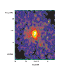
Figure 1.— An adaptively smoothed X-ray image of the gravitational lens system Q0957+561. To improve the signal-to-noise of the lens cluster we selected X-rays with energies ranging between 0.5 and 3 keV. The lens cluster is resolved and appears to be centered slightly northeast of image B. The contour levels are 0.1, 3.5$\times$ 10^-4, 3.5$\times$ 10^-5, 2.2$\times$ 10^-5, and 1.3$\times$ 10^-5 of the peak emission of image A. The white circles indicate the optical locations of the galaxies in the cluster at z = 0.36. Galaxy positions are taken from Angonin-Willaime et al. (1994). North is up east is left.

Figure 2.— An overlay of the VLA and Chandra images of Q0957+561. The contours represent the radio 3.6 cm VLA image of Q0957+561 provided courtesy of Harvanek et al. (1997). The X-ray and radio data are binned with a bin size of 0${}^{\prime\prime}\!\!.$048 on a side. For presentation purposes the X-ray data are smoothed with a circular Gaussian of radius $\sigma$ = 0${}^{\prime\prime}\!\!.$25 resulting in an effective resolution of $\sigma$ $\sim$ 0${}^{\prime\prime}\!\!.$33. The overlay clearly shows that the shape and angular structure of the X-ray and radio jets are similar. The radio contour levels are 0.11, 3.5$\times$ 10^-2, 1.1$\times$ 10^-2 and 3.5$\times$ 10^-3 of the peak emission of image A. The beam width is 0${}^{\prime\prime}\!\!.$24 $\times$ 0${}^{\prime\prime}\!\!.$17. The X-ray image contains photons with energies ranging between 0.5 and 10 keV. The brightness profiles of the X-ray and radio jets differ significantly as shown more clearly in Figure 3. North is up east is left.

Figure 3.— The radio and X-ray intensity profiles are plotted as a function of angular distance from the core of image A along the jet ridge line. The X-ray profile provides counts in 0${}^{\prime\prime}\!\!.$288 increments integrated $\pm$ 0${}^{\prime\prime}\!\!.$48 perpendicular to the jet ridge line and the radio profile provides the 3.6 cm flux density in 0${}^{\prime\prime}\!\!.$096 increments integrated $\pm$ 0${}^{\prime\prime}\!\!.$48 perpendicular to the jet ridge line. Radio counterparts within 0${}^{\prime\prime}\!\!.$5 of the X-ray bright knots located 4^′′ and 6^′′ from the core are clearly visible. Whereas the angular structure of the X-ray and radio jets are similar, the intensity distributions along the jet appear to be anti-correlated. In particular, the X-ray brightness decreases along the jet, whereas the radio flux density of the knots increases with distance from the core (see text for interpretation).

Figure 4.— (Top panel) The X-ray spectrum of the lens cluster along with the best-fit thermal Raymond-Smith model (see Table 2). The model is consistent with a plasma temperature of $\sim$ 2.1 keV. The detected spectral feature between 0.7 and 0.9 keV (observed-frame) correspond to a redshifted z = 0.36 complex of Fe L lines, confirming the detection of the lens cluster. The uncertainty in the calibration of ACIS S3 below 0.5 keV contributes to the large residuals between 0.4 and 0.5 keV. (Lower panel) Residuals in units of standard deviations with error bars of size 1$\sigma$.

Figure 5.— The spectral energy distributions (SEDs) of jet knots B (open circles) and C (filled circles). The radio flux densities were extracted from the radio $\lambda$3.6 cm VLA data kindly provided by Michael Harvanek of Apache Point Observatory. The optical upper limit (cross) is based on published results from a deep HST observation of the field (Bernstein & Fischer 1997). The values of ${\nu}F_{\nu}$ of the jet knots in the X-ray band are at least an order of magnitude above an extrapolation of the radio and optical data points, suggesting that the emission in the radio, optical and X-ray bands is not consistent with a single synchrotron model with a single power law distribution. The solid and dashed lines represent fits of the CMB model (see text) to the spectra of knots B and C, respectively. The CMB model, in which cosmic microwave photons are inverse Compton scattered by synchrotron-emitting electrons in the jet, has the following parameters. Knot B: The emission region is assumed to be spherical with a radius of $R$ = 1 $\times$ 10²³ cm, a magnetic field intensity of $B$ = 6 $\times$ 10^-5 G, and a Doppler factor of $\delta$ = 1.4. The electron distribution is assumed to be a power-law with extremes of $\gamma_{min}$ = 10 and $\gamma_{max}$ = 3 $\times$ 10⁵, a slope of n = 2.6, and a normalization of K = 6.4 $\times$ 10^-5 cm^-3. Knot C: The CMB model for knot C has the same parameters as knot B except K = 4 $\times$ 10^-4 cm^-3 and $\delta$ = 1.05.

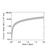
Figure 6.— The total mass of the lens cluster within a radius $r$. The dashed line corresponds to the best-fit spatial and spectral parameters. The shaded region indicates the allowable range of the cluster mass for the estimated uncertainties of the best-fit spatial and spectral parameters.

Figure 7.— The convergence parameter $\kappa$ of the lens cluster as a function of distance from the cluster center. The thick solid line corresponds to the best-fit spatial and spectral parameters. The largest contributor to the uncertainty in the present measurement of $\kappa(x)$ is the weak constraint on the temperature of the cluster. To illustrate this weakness we have plotted the uncertainty in $\kappa(x)$ assuming 68% (dotted lines) and 90% (dashed lines) confidence intervals for the temperature. We also chose cluster limits ranging from 0.7$r_{500}$ and 1.4$r_{500}$, where $r_{500}$ is the radius in which the mean over-density is 500, and $r_{500}$ = 1.58 $h^{-1}_{75}$ Mpc (T_X/10 keV)^1/2 $\sim$ 0.71 $h^{-1}_{75}$ Mpc (Mohr, Mathiesen, & Evrard, 1999). The solid vertical lines indicate the distances of images A and B from the cluster center.