Dynamics of the solar tachocline I: an incompressible study

Abstract

Gough & McIntyre have suggested that the dynamics of the solar tachocline are dominated by the advection-diffusion balance between the differential rotation, a large-scale primordial field and baroclinicly driven meridional motions. This paper presents the first part of a study of the tachocline, in which a model of the rotation profile below the convection zone is constructed along the lines suggested by Gough & McIntyre and solved numerically. In this first part, a reduced model of the tachocline is derived in which the effects of compressibility and energy transport on the system are neglected; the meridional motions are driven instead by Ekman-Hartmann pumping. Through this simplification, the interaction of the fluid flow and the magnetic field can be isolated and is studied through nonlinear numerical analysis for various field strengths and diffusivities. It is shown that there exists only a narrow range of magnetic field strengths for which the system can achieve a nearly uniform rotation. The results are discussed with respect to observations and to the limitations of this initial approach. A following paper combines the effects of realistic baroclinic driving and stratification with a model that follows closely the lines of work of Gough & McIntyre.

1 Introduction

The solar tachocline is a thin shear layer located at the top of the radiative zone. It performs the dynamical transition between the differentially rotating convection zone and the nearly uniformly rotating radiative zone (Brown et al., 1989). In a non-rotating fluid, the interface between a convective and a non-convective region is intrinsically complex, and supports dynamical phenomena such as overshoot and gravity-wave generation. Including a background rotation increases the complexity of the system by driving meridional motions at the interface (Mestel, 1953) and by changing the characteristics of convective motions and overshooting plumes, both leading in particular to non-vanishing anisotropic stresses and differential rotation. Finally, the combination of strong shear and anisotropic small-scale motion has been shown to lead sometimes to the enhancement of any seed magnetic field, and to intermittent (or eventually quasi-periodic) magnetic phenomena which could be related to the observed 11-yr magnetic cycle. The position of the tachocline in this unique dynamical interface makes it one of the most complex, and as a result, one of the most interesting regions of the sun.

In recent years, the tachocline has been one of the principal targets of helioseismic observations of the angular rotation profile of the sun. The determination of the thickness of the tachocline is essential to understanding its dynamics. Assuming a variation profile for the angular velocity across the tachocline, throughout the radiative interior and the convection zone, artificial frequency splittings can be reconstructed which are then fitted to the observations. The most recent estimate of the thickness of the tachocline $\Delta$ using this method is the following: $\Delta=(0.039\pm 0.013){\rm R}_{\odot}$ (Charbonneau et al.,1999). An independent method is proposed by Elliott & Gough (1999): they suggest that the discrepancy between the observed sound-speed profile and that obtained from Standard Solar Models could be related to a chemical composition anomaly caused by the mixing of helium within the tachocline layer. By including an additional mixing layer below the convection zone, and comparing the predicted sound speed of this new model to the observations, they calibrate the thickness of the tachocline to be approximately 0.02 ${\rm R}_{\odot}$, assuming the tachocline to be strictly spherical. If the tachocline is thinner but aspherical, this estimate is a measure of the asphericity. Note that observations of light-elements abundances at the surface also suggest that mixing below the convection zone is confined to a shallow layer (e.g. Brun, Turck-Chièze & Zahn, 1999).

It has also been suggested that helioseismic observations could be used to determine the latitudinal structure of the tachocline, in particular whether the width and position of the tachocline vary with latitude. Independent analyses by Gough & Kosovichev (1995) and Charbonneau et al. (1999) suggest that the base of the convection zone and the tachocline (respectively) may be prolate. Charbonneau et al. (1999) also report that no significant variation in the tachocline thickness can be deduced from the observations. Finally, the most recent observational results on the structure of the tachocline concern its dynamical aspect: Howe et al. (2000) suggest that a large-scale oscillation may be taking place across the tachocline with a period of about 1.3 yr, although these results are contested (Basu & Antia, 2001). If assumed to be related to Alfvénic torsional oscillations, this observation could be evidence for the presence of a magnetic field threading the tachocline with a radial component of about 500 G (Gough, 2000).

Owing to the complexity of the dynamics of this region, only a handful of models of the tachocline have been proposed so far. Spiegel & Zahn (1992) pointed out that the shear across the tachocline must be associated with significant thermal fluctuations through a thermal-wind balance. These temperature fluctuations drive meridional motions and propagate the shear deeper and deeper into the radiative zone. In order to avoid this radiative spreading, Spiegel & Zahn proposed an anisotropic turbulence stress-model to suppress the latitudinal shear within a short vertical lengthscale, the strong stratification of the radiative zone providing a natural explanation for the anisotropy of the small-scale flow. However, it was later argued that such a model cannot adequately describe the tachocline (Gough, 1997, Gough & McIntyre, 1998). Broadly speaking, the strong restriction of turbulent motions to spherical shells by the background stratification in the radiative zone leads to Reynolds stresses that transport not angular momentum but potential vorticity (see Garaud, 2001a, for instance). These Reynolds stresses would therefore drive the system away from rather than towards uniform rotation. Moreover, Spiegel & Zahn’s model of the tachocline assumes that the tachocline is turbulent; it is not clear whether this is indeed the case. The tachocline is likely to be stable (Charbonneau, Dikpati & Gilman, 1999) or marginally stable (Garaud, 2001a) to hydrodynamical linear shear instabilities. However, by assuming the existence of a relatively strong toroidal field, it was shown that MHD 2-D instabilities exist (Dikpati & Gilman, 1999) and can have a significant influence on the redistribution of angular momentum (Cally, 2001).

One of the most natural models for the solar interior rotation, and in particular the quenching of the shear, is to assume the existence of a large-scale primordial field in the radiative zone. Indeed, as the magnetic diffusion timescale in the radiative zone is much larger than the rotation timescale, Ferraro’s isorotation law (1937) ensures that the angular velocity is constant on field lines. Mestel & Weiss (1987) suggested that large-scale fields of amplitude as low as $10^{-3}-10^{-2}$G should be capable of suppressing most of the rotational shear deep in the solar radiative interior. Simulations performed by Rüdiger & Kitchatinov (1997) and MacGregor & Charbonneau (1999) looked at the interaction between a large-scale field with a fixed poloidal component and a purely azimuthal flow. These seemed to confirm this estimate, and indeed managed to reproduce the confinement of the shear to a thin tachocline. However, as it was pointed out by Gough & McIntyre (1998), the very low magnetic diffusivity of the radiative zone enables a strong nonlinear coupling between the thermally driven meridional flows described by Spiegel & Zahn and the large-scale interior field. This interaction is essential to the dynamics of the tachocline. Starting from this idea, Gough & McIntyre (1998) presented the first model of the tachocline to take into account self-consistently the nonlinear interaction between thermally driven meridional flows and a large-scale magnetic field. The complexity of the resulting model, however, precluded the derivation of a complete solution.

It is the purpose of this work to create a model of the tachocline which encompasses gradually more realistic physics, to reproduce eventually the idea proposed by Gough & McIntyre. Only this type of gradual approach can provide an adequate procedure to isolate different dynamical phenomena and to study them individually before combining them into one complex system. In this first paper, the compressibility of the fluid is neglected (as well as the background stratification and the energy transport), in order to study specifically the nonlinear interaction between the magnetic field and the fluid motions. As a result, meridional motions must be driven artificially. This can be done through Ekman-Hartmann pumping on the boundary representing the interface with the convection zone, which has the main advantage of providing a well-known, controlled flow pattern. This idea is discussed in detail in Section 6.3. Subsequent work will study the effects of stratification as well as advective and diffusive heat transport on the system, which can then provide a realistic quantitative description of a thermally driven flow and ultimately of the tachocline.

The initial model studied in this first paper, is presented in Section  2: the assumptions and boundary conditions are discussed and applied to the system, and the numerical procedure for the solution of the governing equations is outlined. In Section 3, the numerical procedure is tested by studying a non-magnetic case. The simulations are compared to the well-known Proudman-Stewartson solution for an incompressible fluid between two concentric rotating spheres (Proudman, 1956, and Stewartson, 1966). The results of the simulations in the magnetic case are presented in Section 4. It is shown that the effects of angular-momentum advection and poloidal-field advection by the meridional flow are essential to the dynamics of the system, thereby emphasizing the importance of correctly taking both into account in realistic models of the tachocline. In particular it is shown that, contrary to common expectations, increasing the amplitude of the magnetic field does not necessarily reduce the amount of shear in the radiative zone. Instead, the simulations presented in Section 4 reveal the existence of three typical regimes, with low-, high- and intermediate-field-strength; only the intermediate regime is able to reproduce the qualitative features of the tachocline. Section 5 presents two boundary-layer analyses which apply locally to different field configurations; the analytical solutions are compared to the numerical simulations. Finally, the simulations are analysed and discussed in Section 6 with respect to previous work and to observations.

2 The model

The principal aim of this study is to try to reproduce the observed rotation profile of the sun in the region below the convection zone, and in particular

1. the sharp transition (within a thin shear layer of thickness no larger than 4 % of the solar radius) between the latitudinal shear observed at the base of the convection zone and the uniform rotation of the radiative interior.

2. the value of the interior angular velocity $\Omega_{\rm c}$ (observed to be about 93% of the surface equatorial angular velocity $\Omega_{\rm eq}$).

Moreover, the model should also aim to reproduce the confinement of the material mixing to the region of the tachocline, as suggested by helioseismic measurements (Elliott & Gough, 1999) and surface light-elements abundances (Brun, Turck-Chièze & Zahn, 1999).

2.1 The assumptions

The model presented in this paper essentially follows the idea proposed by Gough & McIntyre (1998) by assuming the existence of a large-scale primordial field in the radiative zone and looking at its nonlinear interaction with fluid motions (both azimuthal and meridional) near the bottom of the convection zone in particular. In order to do so, nonlinear MHD equations are solved, in a first instance assuming that the fluid is incompressible (this paper) and in subsequent papers in an anelastic approximation of a compressible fluid. This gradual increase in the complexity of the phenomena studied allows the independent study of the nonlinear interaction of the field and the meridional flow on the one hand, and the effects of heat transport and stratification on the other hand. The principal shortfall of the incompressibility assumption is that the mechanisms driving the meridional motions as described by Spiegel & Zahn (1992) are absent from this first model; instead, they are replaced by a judicious choice of boundary conditions which lead to Ekman-Hartmann pumping of a qualitatively similar flow (see Section 6.3).

Two principal simplifications are performed on the system to reduce it to a numerically tractable problem: it is assumed that the system is axisymmetric and is in a steady state. Axisymmetry is a wholly unjustified, albeit standard assumption, which allows a drastic simplification of the MHD equations. The steady-state assumption, on the other hand, is reasonably well justified provided all dynamical timescales (for the rotation and the meridional circulation) are much shorter than the stellar-evolution timescale (which ensures that the background stratification does not vary during the fluid motion), the magnetic-braking timescale (which ensures that the external torques exerted on the system are small), or the magnetic-diffusion timescale (which ensures that the amplitude of the interior field does not vary significantly during the fluid turnover time).

In the following, it will always be assumed that the tachocline lies completely in the stably stratified radiative zone, which agrees reasonably well with observations (Charbonneau et al. 1999). It will also be assumed that the rotation profile in the convection zone is independent of the tachocline dynamics so that the convection zone can be taken as a boundary condition of the model. Finally, it will be assumed that the region studied is located sufficiently far below the region of influence of the solar dynamo (Garaud, 1999) to avoid complications linked with the unsteady character of the dynamo field. As a result of this assumption, the region studied is also likely to be located below the overshoot region.

Within this framework, the system studied is limited to the radiative zone, in a region located between two concentric spherical boundaries, the outer one near the base of the convection zone $r_{\rm out}=r_{\rm c}$, where $r_{\rm c}=0.7{\rm R_{\odot}}$, the inner one at a radius $r_{\rm in}=0.35r_{\rm c}$. The inner core (occupying $r<r_{\rm in}$) is cut out of the region of the simulation to avoid singularities at the origin; the position of the inner boundary should not have a significant influence on the results. The numerical value of $r_{\rm in}$ is chosen in such way as to facilitate the comparison of these simulations with the work of Dormy, Cardin & Jault (1998), who solved a similar system of equations and boundary conditions for geophysical applications.

2.2 The equations

If the fluid motions are assumed to be axisymmetric and incompressible, the MHD equations in a frame rotating with angular velocity $\mbox{\boldmath$\Omega$}_{\rm c}=\Omega_{\rm c}{\hat{\mbox{\boldmath$e$}}_{z}}$ are the following:

$$2\rho\mbox{\boldmath$\Omega$}_{\rm c}\times\mbox{\boldmath$u$}+{\mathbf{\nabla}}p+\rho\mbox{\boldmath$g$}_{\rm h}-\mbox{\boldmath$j$}\times\mbox{\boldmath$B$}-\rho\nu{\mathbf{\nabla}}^{2}\mbox{\boldmath$u$} = 0\mbox{ ,}$$

$${\mathbf{\nabla}\times}(\mbox{\boldmath$u$}\times\mbox{\boldmath$B$})+\eta{\mathbf{\nabla}}^{2}\mbox{\boldmath$B$} = 0\mbox{ ,}$$

$${\mathbf{\nabla}\cdot}\mbox{\boldmath$u$} = 0\mbox{ ,}$$

$${\mathbf{\nabla}\cdot}\mbox{\boldmath$B$} = 0\mbox{ .}$$ (1)

where the nonlinear terms in the meridional circulation $(\mbox{\boldmath$u$}\cdot{\mathbf{\nabla}})\mbox{\boldmath$u$}$ are neglected (it is verified a posteriori that this is a good approximation – see Section 6.3), and $\mbox{\boldmath$g$}_{\rm h}=g_{\rm h}(r){\hat{\mbox{\boldmath$e$}}_{r}}$ is the gravitational acceleration associated with the hydrostatic background. The angular velocity $\Omega_{\rm c}=2.84\times 10^{-6}$ s^-1 is chosen to take the observed interior angular velocity of the sun; $B$ is the magnetic field (with components ($B_{r},B_{\theta},B_{\phi}$)), $j$ is the electric current, and $u$ is the circulation which has components $(u_{r},u_{\theta},u_{\phi})$. In order to derive these equations, the density $\rho$ is assumed to be constant ($\rho_{0}=1$g cm^-3) everywhere, as is the kinematic viscosity $\nu$ and the magnetic diffusivity $\eta$. This approximation is made to simplify the numerical procedure slightly, but can easily be removed. Since, as it will be shown later, the typical values of the viscosity and magnetic diffusivity used in the simulations are several orders of magnitude larger than in the sun, it seems pointless to try and represent accurately the variation of these quantities in this first analysis.

Using the following new system of units:

$$\left[r\right]=r_{\rm c}\mbox{ , }\left[t\right]=1/\Omega_{\rm c}\mbox{ , }\left[B\right]=B_{0}\mbox{ , }[u]=r_{\rm c}\Omega_{\rm c}\mbox{ ,}$$ (2)

where $B_{0}$ is the typical strength of the radial field in the interior, the equations become:

$$2{\hat{\mbox{\boldmath$e$}}_{z}}\times\mbox{\boldmath$u$} = -{\mathbf{\nabla}}p-\mbox{\boldmath$g$}_{\rm h}+\Lambda\mbox{\boldmath$j$}\times\mbox{\boldmath$B$}+E_{\nu}{\mathbf{\nabla}}^{2}\mbox{\boldmath$u$}\mbox{ ,}$$

$${\mathbf{\nabla}\times}(\mbox{\boldmath$u$}\times\mbox{\boldmath$B$}) = -E_{\eta}{\mathbf{\nabla}}^{2}\mbox{\boldmath$B$}\mbox{ ,}$$ (3)

with

$$\Lambda=\frac{B_{0}^{2}}{\rho_{0}\Omega_{\rm c}^{2}r_{\rm c}^{2}}\mbox{, }E_{\nu}=\frac{\nu}{\Omega_{\rm c}r_{\rm c}^{2}}\mbox{ and }E_{\eta}=\frac{\eta}{\Omega_{\rm c}r_{\rm c}^{2}}\mbox{ ,}$$ (4)

where all the quantities are now dimensionless and ${\hat{\mbox{\boldmath$e$}}_{z}}$ is the unit vector parallel to the rotation axis. The Ekman numbers $E_{\nu}$ and $E_{\eta}$ represent the ratios of the rotation timescale to the diffusive timescales, and the Elsasser number $\Lambda$ is the ratio of the typical amplitude of the Lorentz force to that of the Coriolis force. The system is solved for $(u_{r},u_{\theta},u_{\phi})$ and $(B_{r},B_{\theta},B_{\phi})$ by solving the azimuthal component of the momentum equation, the azimuthal component of the vorticity equation, the integrated induction equation and the azimuthal component of the induction equation, together with the mass conservation equation and the solenoidal condition; those equations are

$$2({\hat{\mbox{\boldmath$e$}}_{z}}\times\mbox{\boldmath$u$})_{\phi} = \Lambda(\mbox{\boldmath$j$}\times\mbox{\boldmath$B$})_{\phi}+E_{\nu}({\mathbf{\nabla}}^{2}\mbox{\boldmath$u$})_{\phi}\mbox{ ,}$$

$$2\left[{\mathbf{\nabla}\times}({\hat{\mbox{\boldmath$e$}}_{z}}\times\mbox{\boldmath$u$})\right]_{\phi} = \Lambda\left[{\mathbf{\nabla}\times}(\mbox{\boldmath$j$}\times\mbox{\boldmath$B$})\right]_{\phi}+E_{\nu}({\mathbf{\nabla}}^{2}\mn@boldsymbol{\omega})_{\phi}\mbox{ ,}$$

$$u_{r}B_{\theta}-u_{\theta}B_{r} = E_{\eta}j_{\phi}\mbox{ ,}$$

$$\left[{\mathbf{\nabla}\times}(\mbox{\boldmath$u$}\times\mbox{\boldmath$B$})\right]_{\phi} = -E_{\eta}({\mathbf{\nabla}}^{2}\mbox{\boldmath$B$})_{\phi}\mbox{ ,}$$

$${\mathbf{\nabla}\cdot}\mbox{\boldmath$u$} = 0\mbox{ ,}$$

$${\mathbf{\nabla}\cdot}\mbox{\boldmath$B$} = 0\mbox{ ,}$$ (5)

where $\mn@boldsymbol{\omega}={\mathbf{\nabla}\times}\mbox{\boldmath$u$}$ is the vorticity.

2.3 The boundary conditions

In this first analysis, the boundary conditions chosen for the system are the simplest possible ones that still guarantee the existence of a solution; as a result, they are not necessarily the most accurate representation of the dynamics of the sun (and in particular of the interface of the tachocline with the convection zone). The effects of the boundary conditions on the system, and possible improvements, are discussed in Section 6.3

Figure 1: Boundary conditions.

The boundary conditions are summarized in Fig. 1; the MHD equations presented in equations (5) are solved in a region located between two spherical boundaries, impermeable and no-slip boundaries so that the radial and the latitudinal components of the circulation vanish on the boundaries, and the azimuthal component of the circulation is given by the rotation of the boundaries. As a result, the angular-velocity perturbation is $\tilde{\Omega}=\Omega_{\rm in}-\Omega_{\rm c}$ on the inner boundary where $\Omega_{\rm in}$ is an eigenvalue of the problem (see below) and $\tilde{\Omega}=\Omega_{\rm cz}(\theta)-\Omega_{\rm c}$ on the outer boundary, where

$$\Omega_{\rm cz}(\theta)=\Omega_{\rm eq}(1-a_{2}\mbox{ }{\rm cos}^{2}\theta-a_{4}\mbox{ }{\rm cos}^{4}\theta)$$ (6)

and $\Omega_{\rm eq}=1.07\Omega_{\rm c}$, $a_{2}=a_{4}=0.15$ (according to the observations presented by Schou et al. (1998)). On the equatorial plane, symmetry arguments determine the behaviour of the solutions: $u_{\theta}=0$, $B_{r}=0$, $\partial\tilde{\Omega}/\partial\theta=0$ and $B_{\phi}=0$. On the poles, regularity conditions impose $u_{\theta}=0$, $B_{\theta}=0$, $\partial\tilde{\Omega}/\partial\theta=0$ and $B_{\phi}=0$. The bounding spheres are assumed to be imperfectly conducting and the region outside $[r_{\rm in},r_{\rm out}]$ supports no fluid motion, which implies that the field in that region satisfies ${\mathbf{\nabla}}^{2}\mbox{\boldmath$B$}=0$, with conditions that $\mbox{\boldmath$B$}\rightarrow 0$ at infinity, and that the field structure becomes purely dipolar as $r\rightarrow 0$. The amplitude of the radial component of the field near the poles is fixed such that $B_{r}(r_{\rm in},\theta=0)=B_{0}$. This uniquely determines the boundary conditions for the magnetic field, as a relation between $B_{r}$ and $B_{\theta}$ on the one hand, and between $B_{\phi}$ and $\partial B_{\phi}/\partial r$ on the other hand. As a result of these conditions, when the system is not rotating, the solution for the magnetic field is a purely poloidal dipolar structure with a field strength varying as $1/r^{3}$. When the system is rotating, these boundary conditions drive a meridional flow through Ekman-Hartmann pumping. This flow is used to mimic the baroclinicly driven flow predicted to occur in the tachocline (Spiegel & Zahn, 1992, Gough & McIntyre, 1998), in order to study its interaction with the imposed magnetic field. The principal caveat of this approach is that the typical velocities of the meridional flow scales with $E_{\nu}$ and $E_{\eta}$ as an Ekman-Hartmann flow rather than as a thermally driven flow (i.e. with $u_{\theta}\sim r_{\rm c}\tilde{\Omega}$ and $u_{r}\sim\delta_{\rm EH}\tilde{\Omega}$ where $\delta_{\rm EH}$ is the Ekman-Hartmann boundary-layer thickness). This discrepancy should influence quantitative predictions of the model only whilst leaving qualitative results unaffected.

One of the main aims of this study is to be able to predict the angular velocity of the interior. In order to do so, the angular velocity of the inner core $\Omega_{\rm in}$ is treated as an eigenvalue of the problem, and an additional boundary condition is imposed on the system accordingly, namely that no net torque is applied to the region interior to $r=r_{\rm in}$ (this is a necessary condition to guarantee a steady state). This condition, which determines uniquely the value of $\Omega_{\rm in}$, is equivalent to requiring that the integral of the angular-momentum flux through the boundary vanishes:

$$\int_{0}^{\pi/2}\left(\rho\nu r^{2}\mbox{ }{\rm sin}^{2}\theta\frac{\partial\Omega}{\partial r}+r\mbox{ }{\rm sin}\theta B_{r}B_{\phi}\right)\mbox{ }{\rm sin}\theta{\rm d}\theta=0\mbox{ .}$$ (7)

One can notice through this expression the main justification for choosing conducting boundary conditions: when the region below $r_{\rm in}$ is insulating, the radial component of the current (and thereby the toroidal field) must vanish on the boundary; in that case the angular-momentum flux through the boundary would be purely viscous. Since viscous stresses are normally thought to be negligible in the sun, such a model would be a poor representation of the dynamical structure of the radiative zone.

2.4 Numerical method

The system of equations (5) and the boundary conditions presented in Section 2.3 constitute a well-posed partial differential equations system with one eigenvalue. The numerical method chosen for the solution of this system is the following:

1. to write the system of equations with respect to a spherical polar coordinate system, respecting the symmetry of the problem as well as the regularity conditions on the poles,

2. to expand the latitudinal dependence of the equations into Fourier modes of $\theta$, or equivalently Chebishev polynomials $T_{n}(\mbox{ }{\rm cos}\theta)$,

3. to solve the resulting ODEs and algebraic equations with respect to the independent variable $r$ using a Newton-Raphson relaxation method.

A more detailed description of the numerical procedure can be found in the work by Garaud (2001b).

Manual mesh-stretching is preferred over automatic mesh-point allocation, as the latter was found to have low performance for boundary-layer thicknesses order of $10^{-6}(r_{\rm out}-r_{\rm in})$ or less. This low performance is probably due to the fact that as many Fourier modes are used, the allocation algorithms that were tried cannot choose adequately according the most relevant function against which the mesh should be stretched. When stretching the mesh manually (according to the width and positions of the boundary layers determined in Section 5), a minimum of a hundred points is allocated to each of the boundary layers. Typically, another 200-400 points are allocated to the interval outside the boundary layers, depending on the simulations.

3 Results in the non-magnetic case

As a first step towards the resolution of the model presented above, a simplified system is solved in which the magnetic field is ignored. The hydrodynamics of a fluid between two concentric impermeable rotating spheres is a relatively well-studied problem, both analytically (since Proudman, 1956) and numerically (see for instance Dormy, Cardin & Jault, 1998); these previous studies can be compared with the results of the non-magnetic numerical solutions obtained with the numerical procedure presented in Section 2.4 to test its accuracy and performance.

3.1 Numerical results

As a example, the solution to the non-magnetic subset of equations (5) with an Ekman number $E_{\nu}=8\times 10^{-6}$ is presented in Fig. 2. When no magnetic field is present, for low enough Ekman number, fluid motion is dominated by Coriolis forces everywhere except in two boundary layers near the spherical boundaries, and in a shear layer at the tangent cylinder. In the bulk of the fluid, angular velocity is more-or-less constant on cylinders: indeed, when viscosity is negligible, the fluid dynamics equations for the incompressible fluid reduce to

$$(\mbox{\boldmath$\Omega$}_{\rm c}\times\mbox{\boldmath$u$})_{\rm\phi}=0\mbox{ ,}$$ (8)

which implies that $u$ must be parallel to the rotation axis, and

$$\left({\mathbf{\nabla}\times}(\mbox{\boldmath$\Omega$}_{\rm c}\times\mbox{\boldmath$u$})\right)_{\rm\phi}=0\mbox{ ,}$$ (9)

which implies that the angular velocity must be independent of $z$ where $z$ is the cylindrical coordinate that runs parallel to the rotation axis (Proudman, 1916, Taylor, 1921). Viscous effects are necessary in the boundary layers to ensure the smooth transition between the rotation profile in the bulk of the fluid and that imposed at the boundaries.

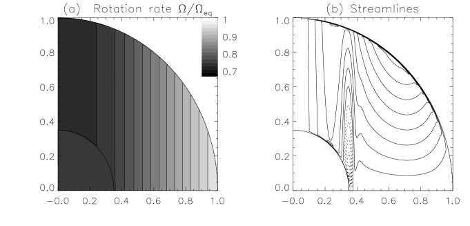
Figure 2: Rotation profile and streamlines in the non-magnetic case for $E_{\nu}=8\times 10^{-6}$. The streamlines are line-coded so that clockwise motions are represented by dotted lines and anti-clockwise motions are represented by solid lines. The interior angular velocity in this simulation is $\Omega_{\rm in}=0.75\Omega_{\rm eq}$.

3.2 Comparison with analytical asymptotic analysis

This structure was first studied by Proudman (1956) and Stewartson (1966), in the case where $E_{\nu}$ is asymptotically small. It is possible to show (see the Appendix) that in this limit the interior angular velocity is uniquely determined by the size of the gap between the two spheres; its value can be predicted analytically, and is given by the following equation:

$$\frac{\Omega_{\rm in}}{\Omega_{\rm eq}}=\frac{\int_{0}^{\pi/2}F(\theta)D(\mbox{ }{\rm sin}\theta){\rm d}\theta}{\int_{0}^{\pi/2}F(\theta){\rm d}\theta}\mbox{ ,}$$ (10)

where

$$F(\theta)=\frac{\mbox{ }{\rm sin}^{3}\theta\mbox{ }{\rm cos}\theta}{\mbox{ }{\rm cos}^{1/2}\theta+\left(1-\mbox{ }{\rm sin}^{2}\theta r_{\rm in}^{2}/r_{\rm out}^{2}\right)^{1/4}}$$ (11)

and

$$D(s)=1-a_{2}\left(1-(s^{2}/r_{\rm out}^{2})\right)-a_{4}\left(1-(s^{2}/r_{\rm out}^{2})\right)^{2}\mbox{ .}$$ (12)

The variation of the calculated value of the interior anguar velocity as a function of the width of the gap $\delta=r_{\rm out}-r_{\rm in}$ is presented in Fig  3.

Figure 3: Analytical prediction for the interior angular velocity as a function of gap width $\delta$, and results of simulations for $\delta=0.5$ and $\delta=0.65$ for values of the Ekman number as shown.

It can be seen that the simulations, represented by the black squares, fit well the analytical predictions provided that the Ekman number is small enough (i.e. below $10^{-6}$). It is also interesting to note, as an aside, that for gap width of about 3% of the radiative zone’s radius (which corresponds to the width of the solar tachocline), the interior angular velocity is 93% of the equatorial velocity, which is very close to the value observed. It is not clear whether this interesting match is a mere fortuitous coincidence or the result of some more subtle physical processes.

Another way of comparing the results of the simulations to analytical predictions is through the construction of the Ekman spiral, which is a parametric representation of the azimuthal velocity against the latitudinal velocity as a function of radius, at a fixed co-latitude $\theta$. Fig. 4 compares the results of the asymptotic solution and the true numerical solution for a slightly different simulation, in which the angular-velocity profile imposed on the outer boundary is chosen to be constant with value $\Omega_{\rm out}=\Omega_{\rm c}+10^{-5}$, and the angular velocity of the inner core is simply $\Omega_{\rm in}=\Omega_{\rm c}$ (the no-torque condition is dropped).

Figure 4: Predicted and calculated Ekman spirals. The analytical prediction in shown as a continuous line, whereas the simulations are shown as squares for $E_{\nu}=10^{-4}$ or triangles for $E_{\nu}=6.5\times 10^{-6}$. The inset shows an enlargement of the central area.

Note how the fit of the asymptotic analytical prediction to the numerical solution is valid only provided the Ekman number is small enough. For larger Ekman numbers, viscosity plays a non-negligible role in the dynamics of the fluid outside the boundary layers, invalidating Proudman’s asymptotic analysis. This result has been obtained already by Dormy, Cardin & Jault (1998) who studied the non-magnetic case extensively. The good agreement between the analytical asymptotic solutions and the simulations validates the numerical procedure.

4 Results in the magnetic case

The influence of the magnetic field on the fluid depends essentially on two parameters: the field strength and the magnetic diffusivity. In this section, three regimes are presented for varying Elsasser number at fixed $(E_{\nu},E_{\eta})$. The Elsasser number is then fixed, and in Section 4.2 the dependence of the solution on the magnetic Ekman number is presented.

4.1 Varying the field strength

In these first simulations, only the Elsasser number $\Lambda$ is varied. Note that the definition of $\Lambda$ defined in equation (4) uses the value of the amplitude of the radial component of the magnetic field on the inner boundary. Accordingly, it should normally be defined using the true value of the density at $r=r_{\rm in}$, which in reality is of order of $\rho_{\rm in}=20$ g cm^-3 rather than the chosen uniform value of $\rho_{0}=1$ g cm^-3. As a result of the uniform-density approximation, the values of $\Lambda$ chosen in this work should be interpreted with care and regarded as rough indications rather than precise values. Note also that as the “initial” magnetic field varies as $1/r^{3}$, the typical local Elsasser number near the surface is about 500 times lower than $\Lambda$.

The values of the viscous and magnetic Ekman numbers chosen for these simulations are identical: $E_{\nu}=E_{\eta}=2.5\times 10^{-4}$. This value was chosen for convinience, as it is then easy to obtain solutions for any value of the magnetic field strength.

4.1.1 Low-field case, $\Lambda=1/25$

This first simulation is shown in Fig. 5, which presents the result in the case of a low Elsasser number ($\Lambda=1/25$). This corresponds to $B_{0}=0.25$ T. The local Elsasser number near the surface is of order of $7\times 10^{-5}$.

The structure of the interior angular velocity is dominated by Coriolis forces, and the angular-velocity profile is close to Proudman (cylindrical) rotation, except maybe near the inner core where the influence of a magnetic field can be seen through the slight deviation in the angular-velocity contour lines. Because of the additional Lorentz forces in the momentum equation, the circulation is no more limited to cylindrical surfaces and takes a rather different pattern, with two cells that burrow deeply into the radiative zone. As expected from standard Ekman-Hartmann pumping (see Acheson & Hide, 1973), the typical value of the latitudinal component of the flow near the top boundary is of order of $r\tilde{\Omega}$, i.e. $u_{\theta}\sim 1.5\times 10^{-2}$ in units of $r_{\rm c}\Omega_{\rm c}$. The advection of the poloidal field by the circulation can be seen in Fig. 5(d) where the field lines are dragged equatorwards in the interior and polewards near the top boundary by a strong anticlockwise polar cell. The shear persists throughout the fluid region, and as a result, leads to the winding up of the poloidal field into a relatively strong toroidal field. Typical values of the toroidal field are of order of one tenth of the value of the poloidal field near the core. This structure shows little resemblance with the observations, failing in particular to impose uniform rotation within the fluid region.

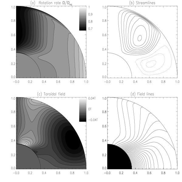
Figure 5: Simulation results for $\Lambda=1/25$, $E_{\nu}=2.5\times 10^{-4}$, and $E_{\eta}=2.5\times 10^{-4}$. Same line-style coding as in Fig. 2 for the streamlines.

4.1.2 High-field case, $\Lambda=25$

The second simulation is shown in Fig. 6, which presents the result in the case of a high Elsasser number. This corresponds to $B_{0}=6.5$ T. The local Elsasser number near the surface is typically of order of $4.5\times 10^{-2}$.

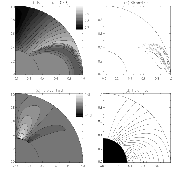
Figure 6: Simulation results for $\Lambda=25$, $E_{\nu}=2.5\times 10^{-4}$, and $E_{\eta}=2.5\times 10^{-4}$. Same line-style coding as in Fig. 2 for the streamlines.

In the strong-field case, (see Fig. 6), the system is essentially dominated by the Lorentz forces everywhere but in diffusive boundary layers. The magnetic field is hardly affected by the circulation, and keeps essentially its dipolar structure everywhere within the fluid region. As a result of Ferraro’s isorotation law, the constant angular-velocity contours follow closely the magnetic field lines. Magnetic connection with the inner core is strong, and a large region within the outermost closed field line near is forced to rotate nearly uniformly with angular velocity $\Omega_{\rm in}$. The matching of this uniformly rotating region to the polar regions and to the outer boundary occurs through a diffusive internal shear layer of thickness $\delta_{\parallel}$

$$\delta_{\parallel}=\left(\frac{E_{\nu}E_{\eta}}{\Lambda_{\rm loc}}\right)^{1/4}\mbox{ ,}$$ (13)

where $\Lambda_{\rm loc}$ is a local Elsasser number, defined with the local value of the typical amplitude of the field instead of $B_{0}$. A more detailed study of this shear layer is outlined in Section 5.2, and presented by Kleeorin et al. (1997), Dormy, Cardin & Jault (1998) and Dormy, Cardin & Soward (2001).

In the polar regions, the field lines are anchored into the differentially rotating convection zone and the latitudinal shear is transmitted to the radiative zone through Ferraro isorotation. The matching of the rotation profile in the polar regions with the outer boundary and the inner core is ensured by the existence of a diffusive Ekman-Hartmann layer with thickness $\delta_{\perp}$ such that

$$\delta_{\perp}=\left(\frac{E_{\nu}E_{\eta}}{\Lambda_{\rm loc}}\right)^{1/2}\mbox{ .}$$ (14)

This boundary layer is discussed in detail in Section 5.1.

The circulation is essentially limited to equatorial regions, with one strong principal cell following the internal shear layer, and weak secondary ones. Again, typical flow velocities along the shear layer are of the order of $r\tilde{\Omega}$ whereas velocities across the layer are of the order of $\delta_{\parallel}\tilde{\Omega}$. This flow is however too slow to have any significant effect on the field. In that case, linear asymptotic analysis can be performed on the system, as shown by Kleeorin et al. (1997). The toroidal field is mostly limited to regions of shear (near the poles) with a very small amplitude in the co-rotating regions. It is worth mentioning that in this case, because the inner regions rotate almost uniformly, relaxing the rigidity condition within $r=r_{\rm in}$ is likely to have little effect on the solution.

4.1.3 Intermediate-field case, $\Lambda=1$

This third simulation is shown in Fig. 8, which presents the result in the case of an intermediate value of the Elsasser number. This corresponds to $B_{0}=1.3$ T. The local Elsasser number near the surface is typically of order of $2\times 10^{-3}$.

The intermediate-field case reveals the emergence of two distinct regions: in the interior the system is dominated by the magnetic field, and is in a state close to uniform rotation, with a large region rotating with angular velocity $\Omega_{\rm in}$ (except in a narrow latitude band around the polar regions). Most of the shear is confined to a thin layer, the “tachocline”; however, within that shear layer and especially near the equator, the system can be observed to follow cylindrical rotation, showing that the system is dominated by Coriolis forces rather than Lorentz forces.

The following phenomenon is happening. A two-cell circulation with upwelling in mid-latitudes is driven by Ekman-Hartmann pumping near the outer boundary, as before. However, in this case the typical circulation velocity ($u_{\theta}\sim r\tilde{\Omega}$) is sufficiently high compared to the Lorentz stresses to advect the magnetic field in a direction parallel to the outer boundary in most latitudes, except near the equator, where it is advected downwards, and near the poles, where the flow is parallel to the field. As a result of this advection process, the amplitude of the radial field on the boundary is everywhere reduced, which confines the field to the radiative zone and diminishes the magnetic connection between the interior field and the imposed latitudinal shear. This can be observed particularly well in Fig. 7, which shows that the radial component of the field is close to zero in the “tachocline” region.

Figure 7: Radial component of the magnetic field as a function of the normalized radius at colatitude $\theta=\pi/3$, for the simulation presented in Section 4.1.3 (i.e. with the parameter values $E_{\nu}=2.5\times 10^{-4}$, $E_{\eta}=2.5\times 10^{-4}$ and $\Lambda=1$) (dotted line), and in Section 4.2 (i.e. with the parameter values $E_{\nu}=6.25\times 10^{-5}$, $E_{\eta}=6.25\times 10^{-5}$ and $\Lambda=1$) (solid line). The dashed line represents the same quantity for a non-rotating system, where the magnetic field solution is a dipolar field decaying as $r^{-3}$.

Moreover the downwards advection of the field in the equatorial regions reduces the value of the local Elsasser number (proportional to the square of the amplitude of the field), which explains the emergence of the cylindrical rotation in that area. Flux conservation implies that the magnetic field strength is correspondingly increased in regions just below. This magnetic field evacuation by the circulation can also be seen in Fig. 10 which shows the square of the amplitude of the magnetic field on the equator as a function of radius. The plot shows particularly well the two regions:

1. in the core, the field is hardly perturbed by the differential rotation imposed on the top, and varies with $r^{-3}$ just as the field would were the system not rotating (as represented by the dashed line).

2. the advection of the field by the circulation can easily be seen near the surface: just below the convection zone, the amplitude of the field is significantly smaller than the initial dipolar field, and slightly lower down the amplitude is correspondingly higher, as required by flux conservation.

Note that the two regions are separated by a magnetic diffusion layer. Additional simulations for different viscous and magnetic Ekman numbers suggest that the thickness of the layer is, as expected, of order of $\delta_{\parallel}$.

Conversely, the magnetic field keeps the circulation from burrowing deep into the radiative zone and confines it to a shallow region. This confinement can be seen in Fig. 8 but is represented best in Fig. 11, which shows the latitudinal component of the velocity as a function of radius. Note how the circulation is heavily suppressed below $r=0.9r_{\rm c}$. Finally, one can see that the polar regions, which are unaffected by the circulation, propagate the slow polar rotation at all radii into the radiative zone, as in the high-field case.

Figure 8: Simulation results for $\Lambda=1$, $E_{\nu}=2.5\times 10^{-4}$, and $E_{\eta}=2.5\times 10^{-4}$. Same line-style coding as in Fig. 2 for the streamlines.

Figure 9: Simulation results for $\Lambda=1$, $E_{\nu}=6.25\times 10^{-5}$, and $E_{\eta}=6.25\times 10^{-5}$. Same line-style coding as in Fig. 2 for the streamlines.

4.2 Varying the magnetic diffusivity

The amplitude of the magnetic field is now set to be that of the intermediate field strength, $B_{0}=1.3T$. When the magnetic diffusivity is decreased by a factor of four, as it is shown in Fig. 9, advection of the magnetic field by the circulation becomes more important compared to diffusion. This has several consequences:

1. the fluid is closer to being a perfect fluid, driving the the system closer to isorotation. A larger volume of fluid in the interior is rotating nearly uniformly with the interior angular velocity and the slow rotating polar regions are confined within a smaller latitude band;

2. the field confinement and the reduction of magnetic stresses is more efficient, as can be seen in Fig. 7 and Fig. 9.

3. as can be seen in Fig. 9 and Fig. 10 the magnetic evacuation in the surface equatorial regions is also greater, and occurs more abruptly as expected. The typical width of the transition layer between the magnetically dominated interior and the magnetic free tachocline seems to vary as $(E_{\nu}E_{\eta})^{1/4}$, confirming that it is a simple magnetic diffusion layer of the type analysed in Section 5.2;

4. as a result, the circulation is confined within a smaller volume by the magnetic field (see Fig. 9 and Fig. 11).

Figure 10: Normalized square of the amplitude of the magnetic field on the equator as a function of normalized radius for the simulation presented in Section 4.1.3 (i.e. with the parameter values $E_{\nu}=2.5\times 10^{-4}$, $E_{\eta}=2.5\times 10^{-4}$ and $\Lambda=1$) (dotted line), and Section 4.2 (i.e. with the parameter values $E_{\nu}=6.25\times 10^{-5}$, $E_{\eta}=6.25\times 10^{-5}$ and $\Lambda=1$) (solid line). The dashed line represents the same quantity for a non-rotating system, where the magnetic field solution is a dipolar field decaying as $r^{-3}$.

Figure 11: Latitudinal component of the velocity as a function of the normalized radius at colatitude $\theta=\pi/3$, in units of the azimuthal velocity $r_{\rm c}\Omega_{\rm c}$, for the simulation presented in Section 4.1.3 (i.e. with the parameter values $E_{\nu}=2.5\times 10^{-4}$, $E_{\eta}=2.5\times 10^{-4}$ and $\Lambda=1$) (dotted line), and in Section 4.2 (i.e. with the parameter values $E_{\nu}=6.25\times 10^{-5}$, $E_{\eta}=6.25\times 10^{-5}$ and $\Lambda=1$) (solid line).

As mentioned previously, quantitative results of the model cannot provide any serious predictions of the observations (because the inadequate driving mechanism used for the circulation, because of the assumption of incompressibility and uniform density, and because of the gross discrepancy between the real solar diffusivities and the ones used in these simulations). Nonetheless, the calculated interior angular velocity provides an interesting point of comparison between different solutions corresponding to different parameters, and reflects on the various dynamical processes occuring in the radiative zone. Figure 12 shows the predicted ratio of interior to equatorial angular velocities as a function of the Ekman number in the intermediate-field case and high-field case as a function of magnetic Ekman number. Again, the viscous Ekman number is chosen to have the same value as the magnetic Ekman number.

Figure 12: Interior angular velocity as a function of the Ekman number $E=E_{\eta}=E_{\nu}$ for the low field case (triangles), intermediate field case (stars) and the high field case (squares) .

The main reason for the initial decrease in $\Omega_{\rm in}$ with decreasing Ekman number is the following: for this range of magnetic Ekman numbers, the polar regions are hardly affected by the shear expulsion, and rotate with a low angular velocity more or less at all radii. A slowly rotating region, connected to the core via magnetic stresses, necessarily imposes its slow rotation to the inner core, with a stronger connection for lower Ekman number. However, as the Ekman number is decreased past a certain threshold, shear expulsion from the core slowly starts affecting the polar regions and the inner core velocity increases again towards the observed values. Note that the value of the interior angular velocity in the extremely diffusive case is of $96\%$ of the equatorial angular velocity, a value which was predicted by Gough (1985).

5 Comparison with asymptotic analytical analysis

This section focuses on presenting two asymptotic solutions near the spherical boundaries, in the case where the magnetic field is mostly perpendicular to the boundary (which occurs near the poles on the inner boundary) and in the case where the magnetic field is mostly parallel to the boundary (which occurs on the outer boundary near the equator). The boundary layer solutions are then compared with the numerical solutions.

5.1 Analysis of the boundary layer in the polar regions

5.1.1 Analytical derivation of the boundary layer solution

When the magnetic field is mostly perpendicular to the boundary, an Ekman-Hartmann boundary layer develops (see the review by Acheson & Hide (1973)). A derivation of the boundary layer analysis is now repeated for the sake of clarity. Assuming that the magnetic field is essentially perpendicular to the boundary with constant amplitude $B_{0}$, one can write

$$\mbox{\boldmath$B$}=B_{0}{\hat{\mbox{\boldmath$e$}}_{r}}\mbox{ .}$$ (15)

Calling $x=r-r_{\rm in}$, the simplified system of MHD equations in the boundary layer on the inner sphere is

$$2\mu\frac{\partial\psi}{\partial x} = \Lambda\frac{\partial S}{\partial x}+E_{\nu}\frac{\partial^{2}L}{\partial x^{2}}$$

$$-\frac{1}{r_{\rm in}}\frac{\partial\psi}{\partial x} = E_{\eta}\frac{\partial b}{\partial x}$$

$$-2\mu\frac{\partial L}{\partial x} = r_{\rm in}\Lambda\frac{\partial^{2}b}{\partial x^{2}}+E_{\nu}\frac{\partial^{4}\psi}{\partial x^{4}}$$

$$\frac{\partial L}{\partial x} = -E_{\eta}\frac{\partial^{2}S}{\partial x^{2}}\mbox{ ,}$$ (16)

where $\psi$ is the stream function of the fluid flow, such that

$$\mbox{ }{\rm sin}\theta u_{\rm\theta}=\frac{1}{r}\frac{\partial\psi}{\partial r}\mbox{ , }u_{r}=\frac{1}{r^{2}}\frac{\partial\psi}{\partial\mu}\mbox{ ,}$$ (17)

and

$$L=r\mbox{ }{\rm sin}\theta u_{\phi}\mbox{ , }S=r\mbox{ }{\rm sin}\theta B_{\phi}\mbox{ and }b=\mbox{ }{\rm sin}\theta B_{\theta}\mbox{ .}$$ (18)

Grouping these equations yields

$$-4\mu^{2}E_{\eta}^{2}F=\left(\Lambda-E_{\nu}E_{\eta}\frac{\partial^{2}}{\partial x^{2}}\right)^{2}F\mbox{ ,}$$ (19)

where $F$ represents $\frac{\partial^{2}S}{\partial r^{2}}$, $\frac{\partial^{2}b}{\partial r^{2}}$, $\frac{\partial^{2}\psi}{\partial r^{2}}$ or $\frac{\partial L}{\partial r}$. Looking for a solution of the kind $F\propto e^{\gamma_{\perp}x}$ yields

$$-4\mu^{2}E_{\eta}^{2}=\left(\Lambda-E_{\nu}E_{\eta}\gamma_{\perp}^{2}\right)^{2}\mbox{ ,}$$ (20)

and in turn, that $\gamma_{\perp}=\pm(\beta\pm i\alpha)$ where

$$\beta =\left(\frac{\Lambda+\sqrt{\Lambda^{2}+4\mu^{2}E_{\eta}^{2}}}{2E_{\nu}E_{\eta}}\right)^{1/2}\simeq\left(\frac{\Lambda}{E_{\nu}E_{\eta}}\right)^{1/2}\mbox{ , }$$

$$\alpha =\left(\frac{-\Lambda+\sqrt{\Lambda^{2}+4\mu^{2}E_{\eta}^{2}}}{2E_{\nu}E_{\eta}}\right)^{1/2}\ll\beta\mbox{ .}$$ (21)

for small enough $E_{\nu}$ and $E_{\eta}$. The solutions, which must be bounded, can then be written out as

$$Q\simeq Q_{c}e^{-\beta x}+Q_{0}\mbox{ ,}$$ (22)

where $Q$ is either of the quantities $S$, $b$, $L$ or $\psi$, and $Q_{c}$ and $Q_{0}$ are integration constants. Note that the boundary layer thickness $\delta_{\perp}=1/\beta$ is, as expected, the same as the one obtained by MacGregor & Charbonneau (1999) in their open-field calculations.

5.1.2 Comparison with the numerical solutions

In order to compare rigorously the simulations to the analytical solutions derived above, the matching of the solutions obtained in the boundary layer to those in the bulk of the fluid should be performed. However, the solution in the bulk of the fluid, in particular in the polar regions, is dominated by geometric effects (as the latitudinal derivatives are not necessarily negligible) and diffusive effects (as the Ekman numbers used in the simulations are not small enough to justify neglecting the diffusive terms); as a result, it is beyond to scope of this analysis to derive an analytical solution for the solutions in the bulk of the fluid, and therefore attempt such a matching. However, it is still possible to check the qualitative behaviour of the solutions in the boundary layer. Fig. 13 shows the angular momentum function $L$ as a function of the scaled variable $\xi=\beta x=\beta(r-r_{\rm in})$, for three different values of the Ekman numbers. Although the boundary conditions and asymptotic conditions are different for each case, this plots illustrates that the angular momentum function $L$ indeed behaves as $e^{\beta x}$ within the boundary layer (i.e. for values of $\xi$ below unity).

Figure 13: Variation with the scaled variable $\xi$ of the angular momentum function $L$ at fixed co-latitude $\theta=\pi/12$ and fixed Elsasser number $\Lambda=1$, for three different values of the Ekman numbers: $E_{\nu}=E_{\eta}=10^{-3}$ (solid line), $E_{\nu}=E_{\eta}=2.5\times 10^{-4}$ (dashed line) and $E_{\nu}=E_{\eta}=6.25\times 10^{-5}$ (dotted line).

5.2 Analysis of the boundary layer in the equatorial region

5.2.1 Analytical derivation of the boundary layer solution

Near the equator, the asymptotic analysis described in Section 5.1 breaks down, as the magnetic field is advected by the circulation into a a direction parallel to the surface. Another type of boundary layer appears, which is analysed in this section.

Assuming little variation in the latitudinal direction, the magnetic field is approximated by $\mbox{\boldmath$B$}\approx B_{0}{\hat{\mbox{\boldmath$e$}}_{\theta}}$; also, as only the region near the equator is considered, one can set $\mu\approx 0$ in the following analysis. In that case, and in the boundary layer only, the MHD equations can be simplified to

$$\Lambda\frac{B_{0}}{r_{\rm out}}\frac{\partial S}{\partial\mu} = E_{\nu}L^{\prime\prime}$$

$$\frac{B_{0}}{r_{\rm out}}\frac{\partial L}{\partial\mu} = E_{\eta}S^{\prime\prime}\mbox{ ,}$$ (23)

where the primes denote differentiation with respect to $r$. These two equations entirely determine the variation of $L$ and $S$ near the boundary, and can be combined into

$$\frac{\partial^{2}Q}{\partial\mu^{2}}=r_{\rm out}^{2}\frac{E_{\nu}E_{\eta}}{\Lambda B_{0}^{2}}\frac{\partial^{4}Q}{\partial\zeta^{4}}\mbox{ ,}$$ (24)

where $Q$ is either $L$ or $S$, and where the boundary layer coordinate $\zeta=r_{\rm out}-r$ was introduced. On the boundary, the latitudinal variation of $L$ is given by the boundary conditions, so that

$$\frac{\partial^{2}L}{\partial\mu^{2}}\approx-2(a_{2}+1)\Omega_{\rm eq}\approx-2(a_{2}+1)L\mbox{ .}$$ (25)

So finally, the governing boundary layer equation is

$$-2(a_{2}+1)L=r_{\rm out}^{2}\frac{E_{\nu}E_{\eta}}{\Lambda B_{0}^{2}}\frac{\partial^{4}L}{\partial\zeta^{4}}\mbox{ ,}$$ (26)

and similarly for $S$. The solutions which are bounded as $\zeta\rightarrow\infty$ are

$$L=L_{c}(\mu)e^{\gamma_{\parallel}\zeta}\mbox{ }{\rm cos}(\gamma_{\parallel}\zeta)+L_{s}(\mu)e^{\gamma_{\parallel}\zeta}\mbox{ }{\rm sin}(\gamma_{\parallel}\zeta)\mbox{ ,}$$ (27)

and similarly for $S$, with

$$\gamma_{\parallel}=\left(\frac{\Lambda B^{2}_{0}}{2(a_{2}+1)r_{\rm out}^{2}E_{\eta}E_{\nu}}\right)^{1/4}\propto\left(\frac{\Lambda_{\rm loc}}{E_{\eta}E_{\nu}}\right)^{1/4}\mbox{ .}$$ (28)

Note that in the work of Rüdiger & Kitchatinov (1997), the poloidal field is entirely confined within the radiative zone and, as a result, is everywhere parallel to the surface near the boundary. This type of boundary analysis therefore applies also to their results, with the following modification: as their latitudinal field varies as $(1-\zeta)^{q-1}$ near the boundary, it can be shown that the thickness of the magnetic diffusion layer scales as $\gamma_{\parallel}\propto\left(\Lambda_{\rm loc}/E_{\eta}E_{\nu}\right)^{1/(2+2q)}$. The case presented here is recovered with $q=1$.

5.2.2 Comparison with the numerical solutions near the equator

Fig. 14 presents the variation of $(L-L_{\rm in})/(L_{\rm eq}-L_{\rm in})$ on the equator as a function of normalized radius, both for the numerical solution and for the “analytical prediction” given by

$$\frac{L-L_{\rm in}}{L_{\rm eq}-L_{\rm in}}\approx e^{\gamma_{\parallel}(r-r_{\rm out})}\mbox{ ,}$$ (29)

where $L_{\rm in}=r_{\rm in}^{2}\Omega_{\rm in}$. This simulation corresponds to the parameters $E_{\eta}=E_{\nu}=6.25\times 10^{-5}$ and $\Lambda=1$. If higher Ekman numbers are chosen, the asymptotic analysis does not satisfyingly reproduce the solution. One can see that the general shape of the solution is well represented by the exponentially decaying solution with boundary layer width $\delta_{\parallel}=1/\gamma_{\parallel}$.

Figure 14: Variation with normalized radius of $(L-L_{\rm c})/(L_{\rm eq}-L_{\rm c})$ on the equator. The solid line is deduced from the numerical solution presented in Section 4.2 and the dotted line is the exponential solution described in equation (29)

The purpose of this section was to determine an asymptotic solution to the equations in the boundary layers near the inner and outer boundaries. This analysis has been used to optimize the mesh-points allocation procedure, as well as to check the behaviour of the numerical solution in the boundaries.

6 Discussion of the results

6.1 Summary of the results and comparison with previous work

Section 4 studied the interaction of a large-scale magnetic field with fluid motions in the radiative zone when a shear is imposed through magnetic and viscous stresses by the convection zone. Three regimes were studied, which depend on the intensity of the magnetic field. It was shown, by varying the magnetic field strength for a given set of diffusion parameters ($E_{\nu},E_{\eta})$, that there exists only a narrow range of parameters $\Lambda$ that leads to a supression of the shear in the bulk of the radiative zone. When the system is dominated by Coriolis forces $(\Lambda\ll 1)$, the shear extends well into the radiative zone through the Proudman constraint. Moreover, two large circulation cells are driven by Ekman-Hartmann pumping on the boundary, and largely mix the radiative zone. In the opposite situation ($\Lambda\gg 1$) the system is dominated by Lorentz forces, and the effects of meridional motion are negligible. In that case, the magnetic field remains essentially dipolar and the latitudinal shear imposed by the convection zone extends along the field lines into the radiative interior. This system was studied in detail by Kleeorin et al. (1997) and Dormy, Cardin & Jault, (1998), who showed the existence of an internal shear layer along the outermost closed field line “associated with the recirculation of electric currents induced in the Hartmann layer as the internal Stewartson layer is associated with the recirculation of meridional flows generated within the Ekman layers”. The thickness of this internal layer is of order of $\delta_{\parallel}$ (Dormy, Jault & Soward, 2001). Note that in this strong-field case it is clear that the internal rotation profile depends entirely on the structure of the imposed field. This can be deduced from the comparative work of MacGregor & Charbonneau (1999), who show how an open-field structure, where the field lines are anchored in the convection zone, results in a differentially rotating radiative zone, whereas in a confined-field structure the shear can be confined to a thin tachocline.

Finally, for $\Lambda\simeq 1$, it is observed that shear exclusion indeed takes place. In that case, meridional motions significantly distort the poloidal field structure, to confine it gradually to the radiative interior as it was initially suggested by Gough & McIntyre (1998). This confinement results in the reduction of the magnetic stresses connecting the radiative interior to the differentially rotating convection zone, and to the expulsion of the shear by the interior field to a thin shear layer, as in the simulations first presented by Rüdiger & Kitchatinov (1997). However, there exists a fundamental difference between the shear layer (tachocline) thickness and position predicted from the Rüdiger & Kitchatinov and MacGregor & Charbonneau (1999) simulations and the ones presented here. In their model for the confined field, as the field structure is prescribed to the system and the meridional flows are neglected, the position of the magnetic diffusion layer is at the boundary and its width is exactly proportional to $\delta_{\parallel}(B_{0})$, where $B_{0}$ is the imposed value of the latitudinal field at the boundary. In the simulations presented here, it is shown that the meridional motions can affect significantly the strength and the geometry of the field near the top of the radiative zone through advection processes, which controls the position and thickness of the magnetic diffusion layer. This phenomenon is intrinsically linked with the nonlinear interaction of the field and the flow and can be studied only through the resolution of the nonlinear MHD equations. The influence of the flow on the field depends also on the strength and on the geometry of the flow, which in turn are intrinsically related to the mechanism which drives the flow. These comments naturally build up to the model proposed by Gough & McIntyre (1998).

One of the principal features of the Gough & McIntyre model is their suggestion that the magnetic diffusion layer could be situated below a virtually magnetic-free tachocline (by magnetic-free, they refer more to a system where the influence of the magnetic field in the dynamical equilibrium is negligible than to a system that has no magnetic field at all). This structure would result from the almost complete confinement of the magnetic field within the radiative zone by the meridional motions (except perhaps in a localized upwelling region in mid-latitudes). Although the simulations above cannot reproduce quantitatively the dynamical balance proposed by Gough & McIntyre (as the circulation in this paper is artificially driven by Ekman-Hartmann pumping instead of thermal imbalance), these qualitative features can easily be identified in Fig. 7 and Fig. 10 . The system seems indeed to lead naturally to a magnetically dominated interior and a rotationally dominated tachocline separated by a magnetic diffusion layer of a thickness that is observed to vary as $\delta_{\parallel}$.

6.2 Comparison with observations

The next step of this analysis consists in comparing the numerical simulations with the observations. In this comparison process, it is essential to keep in mind two essential discrepancies between the model and the real sun: the driving mechanism for the meridional flow in these simulations is artificial, so that the typical flow velocities may be erroneous, and the typical Ekman numbers of the simulations are several orders of magnitude larger than in the sun. In the region of the tachocline, assuming that the flow is not turbulent, the magnetic and viscous diffusion coefficients are of order of $\nu=10$cm²s^-1 and $\eta=2\times 10^{3}$cm²s^-1, which implies that

$$E_{\nu}\simeq 10^{-15}\mbox{ and }E_{\eta}\simeq 2\times 10^{-13}\mbox{ .}$$ (30)

The main consequence of these discrepancies is that although the principal features of the interaction between fluid motions and large-scale fields in the sun can be studied through this method, it cannot provide reliable quantitative estimates.

Despite this obvious shortfall, some aspects of the observations can be reproduced in the simulations.

1. For sufficiently low magnetic diffusivity, a large region of the radiative zone is forced to rotate uniformly with the angular velocity of the core; such a uniform angular-velocity profile in the radiative interior is indicated clearly by the observations. The simulations suggest that polar regions seem to rotate with a low angular velocity down to a latitude of about $50^{\circ}$ for $E_{\nu}=E_{\eta}=2.5\times 10^{-4}$, and down to latitudes of about $60^{\circ}$ for $E_{\nu}=E_{\eta}=6.25\times 10^{-5}$: the polar shear is gradually confined to higher and higher latitudes as the magnetic Ekman number is reduced. Helioseismic inversions still have too low a resolution to provide any reliable observations of the polar regions; this numerical model however predicts more slowly rotating fluid in the polar regions deep within the radiative zone, which is a natural feature of the dipolar field configuration (Rüdiger & Kitchatinov 1997, Gough & McIntyre 1998, MacGregor & Charbonneau 1999). Since the most likely configuration for a fossil field is dipolar, this polar feature is a robust prediction of this family of models.

2. A thin boundary layer appears in which most of the shear is contained, particularly in the equatorial regions. The thickness of this shear layer is much larger than the observed thickness of the tachocline, a discrepancy which is again simply related to the high diffusivities adopted here. It is interesting to note, however, that the position of the magnetic diffusion layer predicted by the simulations is deeper in the equatorial regions than at higher latitudes (which is due to the downward advection of the field near the equator); this could be related to observations of the prolateness of the tachocline (Charbonneau et al, 1999).

3. A two-cell meridional circulation is driven below the convection zone by Ekman-Hartmann pumping; this circulation is confined by the large-scale poloidal field to the tachocline region. This result validates the analysis of the sound-speed profile performed by Elliott & Gough (1999) and also relates to the upper limits in the depth of the tachocline mixing suggested by observations of the abundances of light elements in the convection zone (Brun, Turck-Chièze & Zahn (1999)). Again, the simulated depth of penetration of the circulation is much larger than suggested by the observations, a discrepancy which is due to the large diffusivities used for the numerical analysis, and to the assumption of incompressibility: comparison between high- and low-diffusivity cases indeed show a significant reduction of the mixed-layer depth for lower Ekman numbers, and when the background stratification is taken into account, it is observed to impede radial motions dramatically(see subsequent work).

Finally, as mentioned in Section 4.2, a useful point of comparison between different theoretical models and between models and the observations is the value of the interior angular velocity $\Omega_{\rm in}$. Gough (1985) showed that for an incompressible tachocline controlled by viscous effects, $\Omega_{\rm in}=0.96\Omega_{\rm eq}$. MacGregor & Charbonneau (1999) presented simulations in a confined field configuration which show a virtually uniform rotation profile for the radiative zone with $\Omega_{\rm in}=0.97\Omega_{\rm eq}$. The discrepancy with the observed value ($\Omega_{\rm c}=0.93\Omega_{\rm eq}$) is significant, and comparison with the Gough & McIntyre model shows that either meridional motions and the effects of heat transport and stratification are dominant in the dynamics of the tachocline, or that such a class of models cannot reproduce the observations and that very different dynamics are in play (as in the turbulent stress model proposed by Spiegel & Zahn, 1992, or the nonlinear development of MHD instabilities presented by Cally, 2001). The prediction for the angular velocity presented in Fig. 12 are not conclusive when comparing them with observations, as any discrepancy could be attributed to the large diffusivities used in the simulations.

6.3 Discussion of the model

The ultimate aim of this work is to develop a self-consistent dynamical model of the tachocline which can be used to explain the large range of observations available. In order to do so, the idea proposed by Gough & McIntyre is gradually implemented into a numerically solvable nonlinear MHD model. Although previous work on those lines (Rüdiger & Kitchatinov, 1997, MacGregor & Charbonneau, 1999) has already investigated some of the aspects of the interaction of a large-scale field and differential rotation, two essential ingredients to the model remained to be studied carefully:

1. the nonlinear interaction of a meridional circulation and the imposed magnetic field

2. the baroclinic driving of meridional motions and the effects of compressibility and stratification.

This first paper focuses on the first point only by artificially driving a meridional flow with Ekman-Hartmann pumping on the boundaries. It is found that this artificial system reproduces qualitatively (but not quantitatively) most of the aspects of the Gough & McIntyre model, and of the observations. The good qualitative agreement with the Gough & McIntyre model is perhaps surprising, but is simply due to the qualitative similarities between the Ekman-Hartmann flow and the baroclinicly driven flow, in particular with respect to the two-cell structure with upwelling in mid-latitudes. In both cases, the quadrupolar structure of the flow is linked with the transition in mid-latitudes from a negative radial shear to a positive radial shear. When Ekman-Hartmann layers are present on the outer boundary, they naturally drive poleward motions at high latitudes and equatorward motions at low latitudes, with a return flow upwelling in mid-latitudes. In the sun, thermal-wind balance across the tachocline is shown to lead to temperature fluctuations with a minimum in mid-latitudes, which also results in an upwelling in this region (Spiegel & Zahn, 1992).

Another important point concerns one of the principal assumptions of this numerical model: the linearization of the problem with respect to the advection of momentum by the meridional flow. In order to verify that $(\mbox{\boldmath$u$}\cdot{\mathbf{\nabla}})\mbox{\boldmath$u$}$ can indeed be neglected, it is compared in Fig. 15 to the linear term $2{\hat{\mbox{\boldmath$e$}}_{z}}\times\mbox{\boldmath$u$}$ as well as the Lorentz force $\mbox{\boldmath$j$}\times\mbox{\boldmath$B$}$, for the simulation presented in Section 4.2 and in Fig. 9. As assumed, the nonlinear advection term is everywhere much smaller than the Coriolis term, except perhaps in the Ekman-Hartmann layers near $r=r_{\rm in}$ where both Coriolis and advection term vanish (the system is then dominated by the magneto-viscous balance). It is therefore justified to neglect it. A similar comparison can be performed (see Fig. 15) between the vorticity advection term ${\mathbf{\nabla}\times}(\mbox{\boldmath$u$}\cdot{\mathbf{\nabla}}\mbox{\boldmath$u$})$, the background vorticity advection term $2{\mathbf{\nabla}\times}({\hat{\mbox{\boldmath$e$}}_{z}}\times\mbox{\boldmath$u$})$ and the Lorentz stresses ${\mathbf{\nabla}\times}(\mbox{\boldmath$j$}\times\mbox{\boldmath$B$})$; the conclusion is the same.

Figure 15: Lower panel: comparison between the advection term, the Coriolis force and the Lorentz force at co-latitude $\theta=60^{\circ}$ in units of $r_{\rm c}\Omega_{\rm c}^{2}$, for the simulations presented in Section 4.2. Upper panel: comparison between the vorticity advection term, the background vorticity advection and the magnetic stresses at co-latitude $\theta=60^{\circ}$ in units of $\Omega_{\rm c}^{2}$.

Finally, a few more points must also be raised.

1. As mentioned previously, the diffusivities used in the simulations are far higher than in the sun. The principal effect of high diffusivities is to reduce the interconnection between the field and the flow which can significantly change the balance of forces within the fluid region. This discrepancy is forced by numerical solvability and can be reduced at great cpu expense only.

2. The boundary conditions on the magnetic field are found to have significant influence on the problem (MacGregor & Charbonneau 1999). Although the systematic study of the effects of boundary conditions on the system has not been discussed in this paper, it is illustrated, for example, in the comparison between this work and the results of Dormy, Cardin & Jault (1998) who study (in a geophysical application) the effects of an insulating outer boundary; as a result, the structure of the toroidal field in the interior is altered significantly.

3. The boundary conditions near the top boundary (which is the base of the convection zone) poorly represent the dynamical interaction between the flow and field in the tachocline and the convection zone: the convection zone, and to some extent the overshoot region below, is the seat of fully developed turbulence. It does not behave as an impermeable wall to the circulation in the tachocline, or as a uniformly conducting medium to the magnetic field. Moreover, it is for example widely believed that the interface of the tachocline and the convection zone is the seat of the solar dynamo, which is a non-steady magnetic structure oscillating with a 22 yr period. How can this structure be matched with the assumed steady, nearly dipolar field of the interior? The problem was avoided in this work by assuming that the upper boundary of the tachocline lies safely below the region of influence of the dynamo (see Garaud, 1999) and the overshoot region, but this is clearly an over-simplification.

4. This also raises one of the major issues of the dynamics of the tachocline: to what extent can a steady model represent the system? Firstly, how can the interior field be represented by a steady field when part of it diffuses, or is advected away into the convection zone? In the Gough & McIntyre model, the diffusion of the magnetic field out of the radiative zone is impeded by the confining action of the circulation on the poloidal field, which supports the steady-state assumption. However, the upwelling region discussed by Gough & McIntyre (and observed in Fig. 8) drags the poloidal magnetic field into the convection zone, where it could occasionally reconnect. This phenomenon is intrinsically non-steady, although possibly quasi-periodic (as no magnetic flux is lost through reconnection). Secondly, the hydrodynamical stability of the solution to various instabilities (and in particular to non-axisymmetric perturbations) should be assessed. It was shown by Garaud (2001a) that two-dimensional hydrodynamical instabilities are unlikely to be strong enough to have a significant effect on angular-momentum redistribution in the tachocline. However, the stability of the shear flow tends to be upset by the presence of a magnetic field, as suggested by Gilman & Fox (1997), Dikpati & Gilman (1999) and more recently by Cally (2001). In a stratified fluid, the buoyancy of toroidal flux tubes may lead to a magneto-convective instability. Finally, Alfvén waves can propagate along the magnetic field and lead to the presence of either “localized” oscillations, or global torsional oscillations. The combined effect of these instabilities and waves on the flow may be important in redistributing angular momentum within the radiative zone and across the tachocline. This has not been taken into account in this model.

In future work each of these problems must be addressed. The gradual convergence of the system towards lower and lower diffusivities is “merely” a computational challenge, which can in principle be solved. There is hope that for low enough diffusivities the system reaches an asymptotic state which is more-or-less independent of the Ekman parameters. Asymptotic analyses, following the steps of Kleeorin et al. (1998) for instance, may provide a way of by-passing boundary layers in the flow by providing jump-conditions across the layers. This would greatly help reducing some of the numerical difficulties. However, looking at the importance of geometric or nonlinear effects in the system, it is unlikely that an asymptotic analysis could provide a full solution of the problem. The problem of the representation of the dynamical interaction of the tachocline and the convection zone through adequate boundary conditions is a strong theoretical challenge, which will be looked into in the future. The most obvious route is through the inclusion of the convection zone in the computational domain, and the ad-hoc prescription of Reynolds stresses which would lead to the observed rotation profile. But comparing the relative importance of all the points mentionned in this section, it is clear that the next step towards improving the model is through the inclusion of the effects of compressibility, energy transport and stratification on the dynamics of the system, which will allow a correct quantitative representation of the baroclinic driving of the meridional motions as well as the effects of the strong stratification in the radiative zone. This is work which will be presented in a subsequent paper.

7 Conclusion

This paper presents a numerical analysis of the nonlinear interaction between a primordial field and large-scale fluid flows in the solar radiative zone when a latitudinal shear is imposed from the convection zone through a combination of magnetic and viscous stresses.

Within the scope of some simplifying assumptions (axisymetry, steady-state, incompressibility), the presence of a large-scale field in the radiative zone was shown to lead to three dynamical regimes, which depend essentially on the strength of the underlying field. When the Elsasser number is low, the flow is dominated by the Proudman constraint, which enforces a rotation profile roughly constant on cylindrical surfaces throughout most of the radiative zone. When the Elsasser number is high, the magnetic field propagates the shear to a large part of the interior according to the Ferraro isorotation law, and only within the outermost closed field line does one observe uniform rotation. When the Elsasser number is of order of unity, the magnetic field is weak enough to be advected by meridional motions driven by Ekman-Hartmann pumping on the boundary. This advection process stretches the field along the boundary (thereby reducing the magnetic stresses connecting the convection zone and the radiative zone) and pushes the poloidal field deeper into the interior. As a result, the shear is confined to some shallow layer below the convection zone, which can be likened to the tachocline. Conversely, the meridional circulation is kept from burrowing into the radiative zone by the accumulation of magnetic flux below the tachocline.

The structure of the solution in the intermediate-field case is in qualitative agreement with the angular-velocity observations, as well as the predictions of the Gough & McIntyre (1998) model. The simulations also show the presence of efficient mixing in the tachocline which would influence the abundances of chemical elements in that region; this can also be detected observationally (Elliott & Gough, 1999, Brun, Turck-Chièze & Zahn, 1999).

As expected, the quantitative agreement between the model and the observations is poor; this is due on the one hand to the large diffusivities used in the simulations, and on the other hand to some oversimplification of the dynamics involved (through the boundary conditions chosen, and also the assumption of incompressibility, which drive a meridional flow quantitatively different from what one could expect in the tachcoline). Both of these problems will be addressed in future work; in particular, the effects of compressibility will be studied in a following paper.

In conclusion, although the dynamical behaviour of the sun is likely to be far more complex than that of the simulations presented in this paper, it is clear that these simulations can grasp, and explain, some of the fundamental aspects of the dynamics of the observed solar differential rotation. Moreover, they lay a strong basis for future improvements of the models along the lines described above.

Appendix: Asymptotic solution in the non-magnetic case

Following the work of Proudman (1956), the equations

$$({\hat{\mbox{\boldmath$e$}}_{z}}\times\mbox{\boldmath$u$})_{\phi}=E_{\nu}({\mathbf{\nabla}}^{2}\mbox{\boldmath$u$})_{\phi}\mbox{ ,}$$

$$\left[{\mathbf{\nabla}\times}({\hat{\mbox{\boldmath$e$}}_{z}}\times\mbox{\boldmath$u$})\right]_{\phi}=E_{\nu}({\mathbf{\nabla}}^{2}\mn@boldsymbol{\omega})_{\phi}\mbox{ ,}$$ (31)

are first solved in the main body of the fluid, then successively near the bottom and top boundaries. In the main body of the fluid, the viscous stresses are negligible, so that $u$ is independent of $z$, and the solutions are

$$\psi=\psi_{0}(s)\mbox{ and }\chi=\chi_{0}(s)\mbox{ .}$$ (32)

where $\chi$ is defined such that

$$u_{\phi}=\frac{\chi}{r\mbox{ }{\rm sin}\theta}\mbox{ .}$$ (33)

In order to solve the problem near the lower boundary, Proudman introduces the stretched variable $\zeta$ such that

$$\zeta=(r-r_{\rm in})E_{\nu}^{-1/2}\mbox{ }{\rm cos}^{1/2}\theta\mbox{ .}$$ (34)

This recognizes the presence of a boundary layer with thickness $\delta_{\nu}=E_{\nu}^{1/2}\mbox{ }{\rm cos}^{-1/2}\theta$. The equations (31) become, to zeroth order in $E_{\nu}^{1/2}$

$$\frac{\partial^{5}\psi}{\partial\zeta^{5}} = -4\frac{\partial\psi}{\partial\zeta}$$

$$\frac{\partial^{5}\chi}{\partial\zeta^{5}} = -4\frac{\partial\chi}{\partial\zeta}\mbox{ .}$$ (35)

Note that these approximations are not valid near the poles, where latitudinal derivatives may become important, and near the equator, where the thickness of the boundary layer $\delta$ diverges.

Assuming that the whole system is rotating with angular velocity $\Omega_{\rm in}$ so that effectively $\Omega_{\rm c}=\Omega_{\rm in}$ (this only calls for a slight re-definition of the Ekman number), matching with the boundary conditions at the bottom boundary requires that $\chi\rightarrow 0$ as $r\rightarrow 1$, or $\zeta\rightarrow 0$. Moreover, the impermeable boundary condition requires that $\psi=0$ on the boundary, as well as $\partial\psi/\partial\zeta=0$. The solution to equations (Appendix: Asymptotic solution in the non-magnetic case) which fulfills all these boundary conditions, and which is bounded as $\zeta\rightarrow\infty$ is

$$\psi(\zeta,\theta) = \psi_{1}(\theta)\left(1-e^{-\zeta}(\mbox{ }{\rm cos}\zeta+\mbox{ }{\rm sin}\zeta)\right)$$

$$\chi(\zeta,\theta) = \chi_{1}(\theta)\left(1-e^{-\zeta}\mbox{ }{\rm cos}\zeta\right)\mbox{ ,}$$ (36)

where $\psi_{1}(\theta)$ remains to be determined, and

$$\chi_{1}(\theta)=2E_{\nu}^{-1/2}\mbox{ }{\rm cos}^{1/2}\theta\psi_{1}(\theta)\mbox{ .}$$ (37)

As $\zeta\rightarrow\infty$, these functions must match onto the solution obtained previously for the main body of the fluid region so that is then easy to see that one must have

$$\chi_{1}(\theta)=\chi_{0}(r_{\rm in}\mbox{ }{\rm sin}\theta)\mbox{ and }\psi_{1}(\theta)=\psi_{0}(r_{\rm in}\mbox{ }{\rm sin}\theta)\mbox{ .}$$ (38)

This result can be combined with equation (37) and yields the matching condition

$$\chi_{0}(r_{\rm in}\mbox{ }{\rm sin}\theta)=2E_{\nu}^{-1/2}\mbox{ }{\rm cos}^{1/2}\theta\psi_{0}(r_{\rm in}\mbox{ }{\rm sin}\theta)\mbox{ .}$$ (39)

In order to study the boundary layer near the top boundary, another stretched variable is introduced:

$$\xi=(r_{\rm out}-r)E_{\nu}^{-1/2}\mbox{ }{\rm cos}^{1/2}\theta\mbox{ .}$$ (40)

The scaled equations are the same as before (cf equations (35)); the boundary conditions for the stream function are also the same as for the lower boundary when $\chi\rightarrow 0$, but the differential rotation must now match onto that of the convection zone, so that

$$\chi(r=r_{\rm out},\theta)=r_{\rm out}^{2}\mbox{ }{\rm sin}^{2}\theta\tilde{\Omega}_{\rm cz}(\theta)\mbox{ ,}$$ (41)

where

$$\tilde{\Omega}_{\rm cz}(\theta)=\Omega_{\rm eq}(1-a_{2}\mbox{ }{\rm cos}^{2}\theta-a_{4}\mbox{ }{\rm cos}^{4}\theta)-\Omega_{\rm in}\mbox{ .}$$ (42)

The solutions to equations (Appendix: Asymptotic solution in the non-magnetic case) which fulfill these conditions are

$$\psi(\xi,\theta) = \psi_{2}(\theta)\left(1-e^{-\xi}(\mbox{ }{\rm cos}\xi+\mbox{ }{\rm sin}\xi)\right)\mbox{ ,}$$

$$\chi(\xi,\theta) = \chi_{2}(\theta)+2E_{\nu}^{-1/2}\mbox{ }{\rm cos}^{1/2}\theta\psi_{2}(\theta)e^{-\xi}\mbox{ }{\rm cos}\xi\mbox{ , }$$ (43)

with

$$\chi_{2}(\theta)=r_{\rm out}^{2}\mbox{ }{\rm sin}^{2}\theta\tilde{\Omega}_{\rm cz}(\theta)-2E_{\nu}^{-1/2}\mbox{ }{\rm cos}^{1/2}\theta\psi_{2}(\theta)\mbox{ .}$$ (44)

As before, matching with the solution in the main body of the fluid implies that

$$\psi_{2}(\theta)=\psi_{0}(r_{\rm out}\mbox{ }{\rm sin}\theta)\mbox{ and }\chi_{2}(\theta)=\chi_{0}(r_{\rm out}\mbox{ }{\rm sin}\theta)\mbox{ ,}$$ (45)

so that

$$\chi_{0}(r_{\rm out}\mbox{ }{\rm sin}\theta)=r_{\rm out}^{2}\mbox{ }{\rm sin}^{2}\theta\tilde{\Omega}_{\rm cz}(\theta)-2E_{\nu}^{-1/2}\mbox{ }{\rm cos}^{1/2}\theta\psi_{0}(r_{\rm out}\mbox{ }{\rm sin}\theta)\mbox{ .}$$ (46)

Since $\psi_{0}$ and $\chi_{0}$ are functions of $s$ only, the two matching conditions given by equations (39) and (46) can also be rewritten as

$$\chi_{0}(s) =2E_{\nu}^{-1/2}\left(1-(s/r_{\rm in})^{2}\right)^{1/4}\psi_{0}(s)\mbox{ ,}$$

$$\chi_{0}(s) =s^{2}\Omega^{\prime}_{\rm cz}(s)-2E_{\nu}^{-1/2}\left(1-(s/r_{\rm out})^{2}\right)^{1/4}\psi_{0}(s)\mbox{ ,}$$ (47)

where

$$\Omega^{\prime}_{\rm cz}(s) = \Omega_{\rm eq}\left[1-a_{2}\left(1-(s/r_{\rm out})^{2}\right)\right.$$ (48)

$$\left.-a_{4}\left(1-(s/r_{\rm out})^{2}\right)^{2}\right]-\Omega_{\rm in}\mbox{ ,}$$

which can now be solved uniquely as

$$\psi_{0}(s)= \frac{E_{\nu}^{1/2}}{2}\frac{s^{2}\Omega^{\prime}_{\rm cz}(s)}{\left(1-(s/r_{\rm in})^{2}\right)^{1/4}+\left(1-(s/r_{\rm out})^{2}\right)^{1/4}}$$

$$\chi_{0}(s)= \frac{s^{2}\left(1-(s/r_{\rm in})^{2}\right)^{1/4}\Omega^{\prime}_{\rm cz}(s)}{\left(1-(s/r_{\rm in})^{2}\right)^{1/4}+\left(1-(s/r_{\rm out})^{2}\right)^{1/4}}\mbox{ .}$$ (49)

The flow within two spheres is now known analytically everywhere.

Assuming that the sun is in equilibrium, the total torque applied by the convection zone on the radiative interior should be equal to that exerted by the solar wind on the convection zone. Since that torque is extremely small, it is assumed to be null as a first approximation, which is equivalent to requiring that the sun be in a steady state. This condition determines the interior angular velocity $\Omega_{\rm in}$ uniquely.

In the non-magnetic case, the torques applied by the tachocline onto the radiative zone are purely viscous. As a result, the steady-state condition can be rewritten as

$$T_{\nu}(r=1)=2\pi\nu\int_{0}^{\pi/2}\left[r^{3}\mbox{ }{\rm sin}^{2}\theta\frac{\partial\Omega}{\partial r}\right]_{r=1}\mbox{ }{\rm sin}\theta{\rm d}\theta=0\mbox{ ,}$$ (50)

where $T_{\nu}$ is the total viscous torque and $\Omega=\Omega_{\rm in}+(\chi/r^{2}\mbox{ }{\rm sin}^{2}\theta)$ is the total angular velocity at the base of the fluid region. Using the results derived previously, this condition can be rewritten as:

$$\frac{\Omega_{\rm in}}{\Omega_{\rm eq}}=\frac{\int_{0}^{\pi/2}F(\theta)D(\mbox{ }{\rm sin}\theta){\rm d}\theta}{\int_{0}^{\pi/2}F(\theta){\rm d}\theta}\mbox{ ,}$$ (51)

where

$$F(\theta)=\frac{\mbox{ }{\rm sin}^{3}\theta\mbox{ }{\rm cos}\theta}{\mbox{ }{\rm cos}^{1/2}\theta+\left(1-\mbox{ }{\rm sin}^{2}\theta r_{\rm in}^{2}/r_{\rm out}^{2}\right)^{1/4}}$$ (52)

and

$$D(s)=1-a_{2}\left(1-(s^{2}/r_{\rm out}^{2})\right)-a_{4}\left(1-(s^{2}/r_{\rm out}^{2})\right)^{2}\mbox{ .}$$ (53)

References

- [1] Acheson, D. J. & Hide, R., 1973, Rep. Prog. Phys., 36, 159
- [2] Basu, S & Antia, H. M., 2001, MNRAS, 324, 498
- [3] Brown, T. M., Christensen-Dalsgaard, J. Dziembowsky, W. A., Goode, P., Gough, D. O. & Morrow, C. A., 1989, ApJ, 343, 526
- [4] Brun, A. S., Turck-Chièze, S. & Zahn, J.-P., 1999, ApJ, 525, 1032
- [5] Cally, P. S., 2001, Solar Physics, 199, 231
- [6] Charbonneau, P., Christensen-Dalsgaard, J., Henning, R., Larsen, R. M., Schou, J., Thompson, M. J., & Tomczyk, S., 1999, ApJ, 527, 445
- [7] Dikpati, M. & Gilman, P. A., 1999, ApJ, 512, 417
- [8] Dormy, E., Cardin, P. & Jault, D., 1998, Earth & Planetary Sci. Letters, 160, 15
- [9] Dormy, E., Jault, D. & Soward, A. M., 2001, JFM, in press
- [10] Elliott, J. R. & Gough, D. O., 1999, ApJ, 516, 475
- [11] Ferraro, V. C. A., 1937, MNRAS, 97, 458
- [12] Garaud, P., 1999, MNRAS, 304, 583
- [13] Garaud, P., 2001a, MNRAS, 324, 68
-
[14]
Garaud, P., 2001b, PhD Thesis
available from http://www.ast.cam.ac.uk/pgaraud/ - [15] Gilman, P. A. & Fox, P. A., 1997, ApJ, 522, 1167
- [16] Gough, D. O., 1985, in Proceedings of an ESA Workshop, Garmisch-Parkenkirschen, Germany
- [17] Gough, D. O. & Kosovichev, A. G., 1995, Proceedings of the 4th SOHO Workshop, Pacific Grove, California, 1995, ESA SP-376
- [18] Gough, D. O. & McIntyre, M. E., 1998, Nature, 394, 755
- [19] Gough, D. O., 2000, Science, 287, 2434
- [20] Howe, R., Christensen-Dalsgaard, J., Hill, F., Komm, R. W., Larsen, R. M., Schou, J., Thompson, M. J. & Toomre, J., 2000, Science, 287, 2456
- [21] Kleeorin, N., Rogachevskii, I., Ruzmaikin, A., Soward, A. M. & Starchenko, S., 1997, JFM, 344, 213
- [22] MacGregor, K. B. & Charbonneau, P., 1999, ApJ, 519, 911
- [23] Mestel, L., 1953, MNRAS, 113, 716
- [24] Mestel, L. & Weiss, N. O., 1987, MNRAS, 226, 123
- [25] Nakagawa, Y. & Swarztrauber, P., 1969, ApJ, 155, 295
- [26] Proudman, I., 1956, JFM, 1, 505
- [27] Proudman, J., 1916, Proc. Roy. Soc. A, 92, 408
- [28] Rüdiger, G. & Kitchatinov, L. L., 1997, Astr. Nachr. 318, 273
- [29] Schou, J., et al., 1998, ApJ, 505, 390
- [30] Spiegel, E. A. & Zahn, J.-P., 1992, A&A, 265, 106
- [31] Stewartson, K., 1966, JFM, 26, 131
- [32] Taylor, G. I., 1921, Proc. Roy. Soc. A, 100, 114