Prospects for Constraining Cosmology with the Extragalactic Cosmic Microwave Background Temperature

Abstract

Observers have demonstrated that it is now feasible to measure the cosmic microwave background (CMB) temperature at high redshifts. We explore the possible constraints on cosmology which might ultimately be derived from such measurements. Besides providing a consistency check on standard and alternative cosmologies, possibilities include: constraints on the inhomogeneity and anisotropy of the universe at intermediate redshift $z\ ^{<}_{\sim}10$; an independent probe of peculiar motions with respect to the Hubble flow; and constraining the epoch of reionization. We argue that the best possibility is as a probe of peculiar motions. We show, however, that the current measurement uncertainty ($\Delta T=\pm 0.002\,$K) in the local present absolute CMB temperature imposes intrinsic limits on the use of such CMB temperature measurements as a cosmological probe. At best, anisotropies at intermediate redshift could only be constrained at a level of ${}^{>}_{\sim}0.1\%$ and peculiar motions could only be determined to an uncertainty of ${}^{>}_{\sim}311\,$ km s^-1. If the high $z$ CMB temperature can only be measured with a precision comparable to the uncertainty of the local interstellar CMB temperature, then peculiar motions could be determined to an uncertainty of $1101\,(1+z)^{-1}[\Delta T_{CMB}(z)/0.01\,\mbox{K}]~{}{\rm km~{}s}^{-1}$.

PACS numbers: 95.30.Dr, 95.85.Bh, 97.10.Wn, 98.80.-k, 98.80.Bp, 98.80.Es, 98.58.-w, 98.90.+s

I Introduction

Shortly after the discovery [1] of the cosmic microwave background radiation (CMB) it was realized [2, 3] that an extrasolar detection of this radiation had already been made at $\lambda=2.63$ mm [4] in the relative strengths of the 3874.0 Å[R(1)] and 3874.6 Å[R(0)] absorption transitions of cyanogen (CN) in interstellar molecular clouds. The most recent measurement of interstellar CN absorption yields $T_{CMB}=2.729(+0.023,-0.031)\,$K [5, 6]. This provides an important independent calibration point for the local CMB temperature, since it measures the background temperature far from the solar system. Indeed, the interstellar temperature is in excellent agreement with the best COBE local value of $2.725\pm 0.002\,$K [7, 8, 9]. It is also noteworthy that the precision of the interstellar measurement is now approaching the accuracy of the COBE measurement. This raises the interesting question as to whether similarly accurate determinations of the CMB temperature might be possible in extragalactic absorption systems.

II The Data

Indeed, it has now been well demonstrated that the CMB temperature can be measured at high redshifts by using atomic fine-structure transitions in cool absorption-line systems along the line of sight to high-redshift quasars. This endeavor was first pioneered by Bahcall and Wolf [10] who used C II excitations of absorption along the line of sight to PHL 957 to obtain an upper limit of $T_{CMB}<45$K at $z=2.309$. More recent investigations have been based upon the $J=0$, 1, and 2 ground state fine-structure levels of C I. Among other abundant species (e.g. O I, C II, Si II, N II, and Fe II ), C I is perhaps best suited because it has the smallest energy splitting among its fine-structure levels. A recent summary of the possible absorption lines and their relative merits is to be found in [11].

Using C I, Songaila et al. [12], for example, have observed along the line of sight toward QSO 1331+170 and obtained $T_{CMB}=7.4\pm 0.8\,$K at $z=1.776$ consistent with the expected value of 7.57 K. Similarly, Ge, Bechtold and Black [13] have observed toward QSO 0013-004 and obtained $T_{CMB}=7.9\pm 1.0\,$K at z=1.9731, consistent with the expected value of 8.1 K. These measurements, however, must be taken as upper limits as other excitation mechanisms may have contributed to the observed level populations. Recently, however, Srianand, Petitjean, and Ledoux [14] have shown that an absolute temperature measurement at high redshift is possible. In addition to the fine-structure levels of C I in an isolated remote cloud at $z=2.338$, they utilized a detection of several rotational levels in molecular hydrogen to uniquely constrain competing excitation processes. In this way they could deduce an absolute temperature of $10\pm 4$ K, consistent with the expected value of $9.1$ K. Using a similar technique, Levshakov et al. [15] have made a measurement of $T_{CMB}=11.7^{+1.6}_{-2.5}$ K at the highest redshift yet, $z=3.025$. They also obtained an upper limit of $T_{CMB}<15.2$ for a system at $z=4.466$.

A summary of some of the currently available measurements [12, 13, 14, 15, 16, 17] is shown on Figure 1. At present the existing measurements are quite uncertain and most points can only be treated as upper limits. Nevertheless, with forthcoming high resolution spectroscopy on ever larger telescopes, we can perhaps anticipate that accurate determinations of the CMB temperature at high redshifts may be possible in the not too distant future with a precision comparable to or better than the present existing local interstellar measurement. Indeed, we may now be entering a new epoch in which high precision measurements of the CMB temperature in the distant past become a real possibility. Hence, in this paper, we discuss how measurements of the CMB temperature at various redshifts might be useful to constrain cosmological models. We review the possibilities and estimate the ultimate viability of such constraints based upon the current technology for deducing the local CMB temperature.

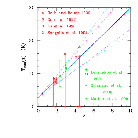
FIG. 1.: Summary of some current measurements of the CMB temperature at various redshifts as labeled. Open symbols are observational upper limits due to the possibility of non-CMB induced excitation. Closed symbols are absolute temperature measurements. The solid line is the extrapolated COBE CMB temperature. Its width is the extrapolated uncertainty for a FRW universe. The dotted lines are the best straight-line fit to the data and the $\pm~{}2\sigma$ uncertainty. The dashed lines are for a power-law fit as described in the text.

Although the data is sparse, it already constrains the possible dependence of the CMB temperature with redshift. Two sets of lines are drawn on Figure 1. One set (dotted lines) corresponds to a straight-line fit (and $\pm 2\sigma$ uncertainty) of the form

$$T(z)=T_{0}(z)(1+bz)~{}~{}.$$ (1)

The other fit (dashed lines) is for a suggested [21] power-law form

$$T(z)=T(0)(1+z)^{1-\beta}~{}~{}.$$ (2)

The fits on these figures are based upon the COBE local measurement plus the two detections of [14] and [15] and the data of [12, 13]. These latter two points are included as a probable detection, though technically they are only an upper limit since alternative excitation processes have not been excluded. These produce limits of $b=0.99\pm 0.22~{}(2\sigma)$ and $\beta=0.003\pm 0.13~{}(2\sigma)$, with $T(0)=2.725\pm 0.002~{}(2\sigma)$ fixed by the COBE measurement. If the data set is limited to only the local COBE point plus the two firm detections [14, 15], then the limits become $b=1.10\pm 0.55~{}(2\sigma)$ and $\beta=-0.05\pm 0.25~{}(2\sigma)$. Clearly, even a few more points could significantly improve the present limits on variations of the CMB temperature with redshift.

From Figure 1 it is clear that given the present day CMB temperature, the standard Friedmann-Robertson-Walker (FRW) cosmology makes a precise prediction of the CMB temperature versus redshift. As long as there has been no significant net heating or dust contamination, and as long as the site of extragalactic CMB measurement is not affected by a large gravitational inhomogeneity (see discussion below) the CMB photon energies are simply redshifted with the cosmic expansion. The near perfect plankian spectral shape of the local observed CMB places very strong constraints on the possibility of contamination by an early epoch of violent star formation or dust. The current COBE limit on the Compton $y$ parameter, $y=\int(kT_{e}/m_{e}c^{2})d\tau<1.5\times 10^{-5}~{}(3\sigma)$ essentially eliminates the possibility of any significant distortions from early star formation/ionization or dust. Hence, to high accuracy one can invoke a simple relation between the cosmic scale factor $a$, the cosmic redshift $z$ and the expected background radiation temperature $T_{CMB}(z)$ for photons arriving from regions that are not too deep within a gravitational potential,

$${T_{CMB}(z)\over T_{CMB}(0)}={a_{0}\over a}=1+z~{}~{},$$ (3)

where $T_{CMB}(0)$ is the present CMB temperature. An accurate measurement of the present CMB temperature thus enables an accurate prediction of the FRW CMB temperature at all redshifts between now $(z=0)$ and the surface of last photon scattering $(z\approx 1100)$.

III Constraining Alternative Cosmologies

Although the temperature-redshift relation of the standard hot big-bang seems well established, a direct observation of the correlation of CMB temperature with redshift is still a useful cosmological probe. At the very least it confirms the notions of entropy conservation and a hotter, denser early universe and helps to eliminate alternative cosmologies [18]. For example, in principle one might still imagine in spite of a number of difficulties (cf. [19]) that a steady-state (or quasi steady-state) cosmology could be contrived [18, 20] to produce a universal 3$K$ microwave by some combination of starlight and dust. However, an increase of the microwave background temperature with redshift is difficult to achieve in such models.

Nevertheless, alternative models have been proposed [21] in which photon creation takes place. In this case the temperature-redshift relation would obey $T_{CMB}(z)/T_{CMB}(0)=(1+z)^{1-\beta}$, where $0\leq\beta\leq 1$. These models therefore give a lower temperature at high redshift. They can only be constrained by direct measurements of the temperature redshift relation. As noted above the current $2\sigma$ limit is $\beta=0.003\pm 0.13$. This is consistent with the existing constraint from big-bang nucleosynthesis [22].

These data also constrain a possible Hoyle-Narlikar cosmology [23] in which the galactic redshift is proposed to result from variations in the electron mass in a flat Minkowski spacetime. In this case, the local background temperature could actually decrease with redshift, though the apparent temperature would be constant. This also is ruled out at the level of $8\sigma$ by the present data.

As a final note, we point out that measurements of the fine structure splitting at high redshift which determine the CMB temperature can also be used to place limits on the possibility of a time varying fine-structure constants [24, 25, 26]. This can happen, for example, in theories that invoke extra compact dimensions to unify gravity and other fundamental forces. The cosmological evolution of the scale factor will then manifest itself [27] as a time dependence of the coupling constants. Another possibility is in unified theories which introduce a new scalar field with couplings to the Maxwell scalar $F_{ab}F^{ab}$. The evolution of the scalar field implies a time variability to $\alpha$ [28].

Any time dependence of the fine structure constant in particular should be apparent in the observed multiplet splitting at high redshift. The relative magnitude $\Delta\lambda/\lambda$ of the multiplet splitting scales as

$${\Delta\lambda\over\lambda}\sim\alpha^{2}$$ (4)

Hence, any limits on the variation of the splitting with redshift also constrains the fine structure constant,

$${\Delta\alpha(z)\over\alpha(z)}\approx{1/2}\biggl{[}{(\Delta\lambda/\lambda)_{z}\over(\Delta\lambda/\lambda)_{0}}-1\biggr{]}~{}~{},$$ (5)

where $\Delta\lambda$ is the wavelength difference between the observed multiplet lines and $\lambda$ is the weighted mean wavelength of the multiplet. The best current limits [24] on a time variation of $\alpha$ are at a level of $|\Delta\alpha/\alpha|\sim 10^{-5}$ based upon multiplet splitting of different species measured simultaneously. The narrow absorption line systems of interest for the CMB measurements of interest here will require a comparable resolution. For C I, the absorption multiplets are split by $\Delta\lambda$ a few hundred $\AA$. Hence, one must resolve the multiplet splitting to $\sim 0.01\AA$ to achieve comparable accuracy.

IV Constraining Anisotropy and Inhomogeneity

Sufficiently accurate CMB temperature measurements could possibly probe the inhomogeneity and anisotropy of the background radiation at redshifts intermediate between the present epoch and the surface of photon last scattering. At present our only information on inhomogeneity and anisotropy of the radiation density are from the surface of last scattering at $z\approx 1100$.

First, imagine an idealized case in which one could make a number of measurements along nearly the same line of sight but at different redshifts, $T_{CMB}(z)$. This might be possible, for example, if enough narrow absorption-line systems exist along the line of sight to a distant quasar. If no other effects were in operation, then the difference in temperature at some location compared with the expected mean FRW temperature $\langle T_{CMB}(z)\rangle$ could be taken as a measure of the inhomogeneity in radiation density along that line of sight,

$${T_{CMB}(z)-\langle T_{CMB}(z)\rangle\over\langle T_{CMB}(z)\rangle}\sim{\Delta\rho\over\rho}~{}~{}.$$ (6)

Although in this case one mainly measures the inhomogeneity of the universe, it is dependent upon several complicating factors as described below.

Similarly, in another idealized situation, assume we have high quality measurements of $T_{0}$, and $T_{i}(z)$ where $T_{i}(z)$ refers to numerous measurements of the background temperature at different points on the sky, but the same observed redshift. There are then at least two more kinds of test that one could do:

One is to measure the mean temperature $\bar{T}(z)$, where,

$$\bar{T}(z)={1\over N}\sum_{i=1,N}T_{i}(z)~{}~{}.$$ (7)

On average one should expect some of the deviations listed below to cancel. If enough points could be obtained at a given $z$, this quantity should agree closely with the FRW prediction. Thus, $\bar{T}(z)$ as a function of $z$ tests the thermal history of the universe. Any deviation of this quantity from the FRW prediction could require a new cosmological paradigm.

Another possible test is the difference $\Delta T(z)=T_{i}(z)-\bar{T}(z)$ at fixed $z$. The difference of the radiation density at distinct points on the sky but fixed $z$ is a measure of some combination of inhomogeneity and anisotropy. As is easily seen from Figure 2, different regions of the last scattering surface are being seen at different redshifts, and thus, the anisotropy of the last scattering surface as seen at points $z_{i}$ is tested. However, the surface of constant $z$ is not necessarily parallel to the surface of last scattering as illustrated in Figure 2. This measure of inhomogeneity and isotropy may be influenced by other factors such as those listed below.

V Effects on the Observed $z-T$ relation

From the above discussion, it is clear that one must carefully identify the dominant influences on the possible deviations of the local microwave temperature from one location to another. The true situation is more complicated than the simple FRW picture especially with regard to detecting any angular anisotropy. We illustrate this in the lightcone structure sketched in Figure 2. From the point of view of observations, it is natural to work with the measured constant-$z$ hypersurfaces sketched by the wavy line on Figure 2. The points $A$ and $B$ represent two points on such a hypersurface, specified by $z=z_{A}=z_{B}$ and the directions $\theta_{A}$, $\phi_{A}$ and $\theta_{B}$, $\phi_{B}$ on the sky.

FIG. 2.: Schematic illustration of the lightcone in a perturbed universe vs. a pure FRW universe.

In an unperturbed FRW universe the hypersurfaces of constant $z=z_{A}=z_{B}$ and constant energy density are obviously equivalent. This is no longer true in a universe perturbed by for example: (i) intrinsic temperature inhomogeneities of the surface of last scattering; (ii) inhomogeneities of the local gravitational potential at $z_{A}$ or $z_{B}$; (iii) inhomogeneities due to the integrated Sachs-Wolfe effect between the surface of last scattering and $z_{A}$ or $z_{B}$; and (iv) peculiar velocities at $z_{A}$ or $z_{B}$. This means that in the real universe, the $z=\,$constant and the last scattering surface (to a first approximation constant energy density) are not “parallel” to each other, i.e. in Figure 2 the points A and B are at the same observed redshift. We digress here to discuss the likely best obtainable measurement error and how this compares with these possible deviations from the expected FRW $z-T$ relation.

A Measurement Error

For a measurement error comparable to that of the local interstellar CMB measurements, $\Delta T_{CMB}(z)\sim\pm 0.02\,$K, one might expect to constrain the anisotropy and inhomogeneity of the universe at a level of

$$\frac{\sigma_{T_{CMB}(z)}}{\langle T_{CMB}(z)\rangle} > \frac{\Delta T_{CMB}(z)}{\langle T_{CMB}(z)\rangle}$$ (8)

$$= \frac{\Delta T_{CMB}(z)}{(z+1)T_{CMB}(0)}=7\times 10^{-3}/(z+1)~{}~{},$$ (9)

corresponding to a level of about 0.2% at a redshift of 3. Even if the only uncertainty could be reduced to the present measurement error of the local CMB temperature propagated to redshift $z$, the best one could hope to do corresponds to a present limit of about 0.1%, i.e.

$$\frac{\sigma_{T_{CMB}(z)}}{\langle T_{CMB}(z)\rangle} > \frac{(1+z)\Delta T_{CMB}(0)}{\langle T_{CMB}(z)\rangle}$$ (10)

$$= \frac{\Delta T_{CMB}(0)}{T_{CMB}(0)}=7.34\times 10^{-4}.$$ (11)

This uncertainty is to be compared with the possible deviations from the pure FRW picture.

B Intrinsic Temperature Fluctuations on the Surface of Last Scattering

There is no reason in standard cosmological models to expect the temperature fluctuations at intermediate redshift to substantially differ from the presently observed fluctuations in the CMB temperature of $\Delta T_{CMB}(0)/T_{CMB}(0)\sim 10^{-5}$. They are therefore probably not detectable. CMB temperature measurements at various redshifts, however, might still constrain exotic cosmological models in which the universe could be postulated to have experienced substantial entropy gain or loss, and/or oscillations at some intermediate ($z^{<}_{\sim}10$) epoch.

C Gravitational Potential at the Absorber

As noted in the introduction, the best place in which to detect the local extragalactic background temperature is probably in cool, narrow absorption-line systems along the line of sight to background quasars. Generally, it is believed [29] that such systems reside in the intergalactic medium in large filamentary flattened structures of low or moderate overdensity. Hence, the local gravitational redshift is probably negligible for such systems.

Nevertheless, one should keep in mind the magnitude of a possible gravitational redshift $\Delta T_{g}/T(z)=z_{g}\approx GM/Rc^{2}$ which might alter the $z-T$ relation. Even for the extreme case of a cloud within a galaxy with $M\approx 10^{12}$ M_⊙ which has been compressed to $R\sim 1$ kpc, the gravitational redshift is only $z_{g}\sim 5\times 10^{-5}$ and thus well below our estimated best observable limits. Similarly, for a large dense galactic cluster one might envision a worst case of a cloud at a distance of only $R\sim 1$ Mpc from a compact galactic cluster of $M\approx 10^{14}$ M_⊙. Even for this extreme case the redshift effect is only $z_{g}\sim 5\times 10^{-6}$, again well below our estimated detection limits.

D Integrated Sachs-Wolfe Effect

For photons which propagate from the surface of last scattering to point $z_{A}$ or $z_{B}$ in Figure 2, there are two ways to think of the Sachs-Wolfe effect [30]. If large-scale departures from homogeneity caused the expansion of the universe to differ along different lines of sight, then this would produce a quadrupole anisotropy. The current COBE limits on the CMR quadrupole anisotropy, however, limit this possibility to an expected amount of $\Delta T/T\sim 10^{-5}$. Hence, this is probably not detectable.

Alternatively, one can view this effect as a correction for the gravitational potential of the mass fluctuation spectrum at the surface of last scattering. This gravitational redshift is expected to be much smaller than the gravitational redshifts described above, i.e. comparable to the intrinsic temperature fluctuations at the surface of last scattering. Indeed, for absorbers at $z>1$, we may expect that this contribution can be neglected. Similarly, the effects of photons crossing gravitational inhomogeneities between the surface of last scattering and the absorber, or between the absorber and the observer, cancel unless the fluctuations are comparable to a Hubble length.

Hence, we conclude that the effects of inhomogeneities in the absorber gravitational potentials or the surface of last scattering are not likely to be detectable by measurements of the CMB temperature at high redshift. Indeed, the only possible observable effects are probably those due to streaming motions, which we now consider in more detail.

VI Probes of Large-Scale Motion

A Dark-Matter Potentials

Perhaps a more useful cosmological constraint could come from using the CMB temperature at intermediate redshifts to probe large-scale peculiar motion. Over 90% of the matter in the universe is dark (invisible). It only manifests itself through gravity. It is important, therefore, to constrain the dark matter potentials through peculiar (i.e., local) motions of galaxies and clusters of galaxies. The matter density fluctuations $\delta$ are related to the peculiar velocities ${\bf v}_{p}$ locally by

$${\bf\nabla\cdot v}_{p}=-f(\Omega)\,\delta,$$ (12)

where $f(\Omega)=d\,\mbox{ln}\delta/d\,\mbox{ln}a\simeq\Omega_{m}^{0.6}$, with $a$ denoting the cosmic scale factor. In principle, it is possible to reconstruct the mass density field from observed peculiar velocities [31]. If peculiar velocities are sufficiently well known, then statistical studies of the peculiar velocity distribution in the universe can be used to constrain cosmological models.

In principle, such peculiar velocities can be determined from measurements of the CMB temperature. If measurement of the CMB temperature at a given redshift can be made sufficiently precise, a comparison of the spectroscopic redshift to the CMB temperature in a distant absorption-line system could be used to detect the line-of-sight component of the absorber’s peculiar motion.

The observed spectroscopic redshift $z_{s}$ for a CMB absorption system is actually the combination of two effects. That is, $1+z_{s}=(1+z)(1+z_{p})$, where $z$ is the cosmic redshift, while $z_{p}$ is the redshift due to the component of peculiar velocity along the observed line of sight [32]. Although the net spectroscopic redshift is dependent upon proper motion, the deduced CMB temperature is almost independent of proper motion. The only effect of proper motion on the background temperature is to produce a dipole moment which averages out in the angle-integrated net population temperature. Thus, the CMB temperature can be used to deduce the true cosmological redshift via equation (1), $z=T_{CMB}(z)/T_{CMB}(z=0)-1$. The peculiar velocity is just c$z_{p}=c(z_{s}-z)/(1+z)$, so that its uncertainty can be written:

$$c\Delta z_{p} = c\,(1+z)^{-1}\sqrt{(1+z_{p})^{2}(\Delta z)^{2}+(\Delta z_{s})^{2}}$$ (13)

$$= c\biggl{\{}(1+z_{p})^{2}\left[\left({\Delta T_{CMB}(z)\over T_{CMB}(z)}\right)^{2}+\left(\frac{\Delta T_{CMB}(0)}{T_{CMB}(0)}\right)^{2}\right]$$ (15)

$$+(\frac{\Delta z_{s}}{1+z})^{2}\biggr{\}}^{1/2},$$

where $\Delta T_{CMB}$ is the uncertainty in the measurement of $T_{CMB}$, and $\Delta z_{s}$ is the uncertainty in the spectroscopic redshift. The error in the observed spectroscopic redshift is usually much less than the error in the CMB temperature and can be neglected. If we assume that a precision comparable to the uncertainty from the local interstellar CMB temperature can be obtained, then this implies a limit to detectable velocities of,

$$c\Delta z_{p}\ ^{>}{}_{\sim}\,\frac{1101}{(1+z)}\,\left[\frac{\Delta T_{CMB}(z)}{0.01\,\mbox{K}}\right]~{}{\rm km~{}s}^{-1}.$$ (16)

Note, that for a given measurement uncertainty $\Delta T_{CMB}(z)$, it is easier to detect peculiar velocities at large $z$, since the Doppler shifted wavelength of the photons, $(1+z_{p})\lambda_{0}$, is shifted an additional factor of $1+z$ due to the expansion of the universe. This effectively amplifies the present signature of the peculiar motion $v=cz_{p}$ at cosmic redshift $z$.

In the limit that the measurement uncertainty could be reduced to as small as the current COBE uncertainty in the local CMB temperature, we would still have $\Delta T_{CMB}(z)\geq(1+z)\,\Delta T_{CMB}(0)$, hence

$$c\Delta z_{p}\ ^{>}{}_{\sim}311\,{\rm km~{}s}^{-1}~{}~{}.$$ (17)

Thus, only large peculiar motions are likely to be detectable by this technique. Nevertheless, there are significant large-scale motions in the universe [33]. In the central parts of rich superclusters, the line-of-sight peculiar velocities of clusters are of order 1200 km s^-1 and can be much larger for individual galaxies [34]. Such clusters are important as tracers of the gravitational potential of the superclusters. The excitation temperature of absorbers in these systems might therefore provide useful constraints on the radial peculiar velocities.

B Distance Calibration

The CMB temperature at small redshifts may also provide support for distance standards. To establish distance ladders to cosmological distances, observers need to calibrate Cepheid variables in nearby galactic clusters. One uncertainty in such calibration has been the relative positions of the Cepheid host galaxies within the clusters. The maximum peculiar velocity corresponds to galaxies located in the center of the cluster. Therefore, if one can measure the peculiar velocity of the host galaxies to sufficient accuracy via the combination of the measurements of the CMB temperature and redshift at the location of a Cepheid host galaxy, one could in principle eliminate the ambiguity in the calibration of Cepheids arising from its location relative to the center of the cluster.

VII Constraining the Epoch of Reionization

The universe was probably reionized at $z^{>}_{\sim}3$. The time scale over which the universe made the transition from being neutral to being almost completely reionized is unknown. Constraints on reionization will help reveal the nature of the first generation of objects that ended the so-called dark ages of the universe. Radio observations of the redshifted 21-cm emission of neutral hydrogen have been proposed [35] as a means to search for the signature of reionization. Basically, one expects a sharp cutoff in the 21-cm emission for the redshift interval corresponding to the epoch of reionization.

We point out that similarly, there should be a sharp drop in the abundance of the neutral atomic and diatomic species of interest here at the epoch of reionization. It is likely, therefore, that CMB-induced C I, O I, CN and CH excitations might be observed at high redshifts (before reionization) and also after reionization at intermediate redshifts (say, $z\sim 2$) but not in between. Whereas the signal from ionized species like C II, Si II, N II, and Fe II may actually increase. Since all of these absorption lines occur at wavelengths around 4000$\,\AA$ in the rest frame, they will be redshifted to the infrared for photons absorbed during the reionization epoch. NGST will be the ideal instrument for detecting such features over a wide redshift range. The existence of a gap in redshift space for the appearance of such features might be an independent means to identify the epoch of reionization.

VIII Observational Feasibility

A Diatomic Absorption Features

While using the atomic fine-structure transitions in C I is a proven method of measuring the CMB temperature at high redshifts [12, 13, 14], the use of the transitions to rotational or fine-structure modes in the diatomic molecules CN, CH, and CH⁺ might still deserve further exploration. Although less abundant, they may provide an alternative and complementary method of measuring the CMB temperature at low and high redshifts. Since they are the preferred absorption features for the local interstellar medium, one might take advantage of ratios to the local interstellar absorption features to minimize systematic error. Hence, we summarize here some of the observational considerations.

The observed equivalent widths of a pair of lines ($i$, $j$) in a molecular cloud, $W_{i}$ and $W_{j}$, are converted into column densities $N_{i}$ and $N_{j}$ assuming a single-component Gaussian curve of growth in each case. Any unresolved structure in the lines will be accurately represented by this approach, provided there are no narrow, heavily saturated, optically thick components whose column densities dominate the composite line-of-sight value [6, 37, 38]. Assuming thermal excitation by the CMB, the ratio of the column densities is given by a Boltzmann factor:

$$\frac{N_{i}}{N_{j}}=\frac{g_{i}}{g_{j}}\,\exp\left(-\frac{h\nu_{ij}}{k_{B}T_{CMB}}\right),$$ (18)

where $g_{i,j}$ are statistical weights of the lower and upper states, and $h\nu_{ij}=E_{i}-E_{j}>0$ is the difference in energy of the two rotational (CN) or fine-structure (CH) states.

To make predictions for the observable equivalent widths at a redshift $z$ for an arbitrary transition $i\rightarrow j$ due to the CMB, we write

$$\frac{N_{i}}{N_{j}}=\frac{g_{i}}{g_{j}}\,\exp\left(-\frac{1\,\mbox{mm}}{\lambda_{ij}}\,\frac{5.278}{1+z}\right),$$ (19)

where $\lambda_{ij}=c/\nu_{ij}$, and we have used $T_{CMB}(z)=2.728(1+z)$. To a good approximation, we can use $W_{i}\propto N_{i}f_{i}\lambda_{i}^{2}$, where $f_{i}$ is the oscillator strength of the transition, and $\lambda_{i}$ is the wavelength of the absorption line. Now we find

$$\frac{W_{i}}{W_{j}}=\frac{g_{i}}{g_{j}}\,\frac{f_{i}}{f_{j}}\,\left(\frac{\lambda_{i}}{\lambda_{j}}\right)^{2}\,\exp\left(-\frac{1\,\mbox{mm}}{\lambda_{ij}}\,\frac{5.278}{1+z}\right).$$ (20)

Clearly, observation of the absorption line from the excited state $i$ is favored by large $\lambda_{ij}$. The smaller $\lambda_{ij}$, the smaller $W_{i}$ relative to $W_{j}$, the more suppressed the absorption line $i$ relative to absorption line $j$. This explains the relative strength of the CN lines (in order of decreasing line strength) R(0), R(1), and the marginal detection of the R(2) line, and the non-detection of the CH line R₁(1) in local measurements [36].

In general, the relative strength of an absorption line from an excited state increases with redshift $z$. Since all of the absorption lines in the strongest interstellar bands of CN have wavelengths of about 4000$\,\AA$, we are restricted to $z<2$ by the wavelength ($\sim 1\,\mu$m) at which optical observations are hindered by atmospheric absorption. However, space-based infrared observations from HST or the upcoming NGST can search for CN and CH excitations at redshifts $z^{>}_{\sim}3$.

For CN, we find $W_{1}/W_{0}=2.00\,\exp[-2/(1+z)]$. This gives $W_{1}/W_{0}=0.27$, close to the observed value of 0.31 for $\zeta$ Ophiuchi. For $z=1$, $W_{1}/W_{0}=0.74$; for $z=2$, $W_{1}/W_{0}=1.03$. These estimates agree with numerical results. Thus, prospects for observing CN excitation at large redshifts is rather good, as long as CN clouds can be found at these redshifts. Although CN absorption from an excited rotational state has not yet been detected outside the Milky Way, observational efforts should be directed toward their detection, since CN has been demonstrated to be an excellent CMB thermometer [5, 6, 39]. Using an approach first explored by Penzias, Jefferts and Wilson [40], Roth et al. [5, 6] directly measured the amount of local excitation from millimeter observations of CN rotational line emission. Once local effects were reliably understood, they were able to make small corrections to the CN excitation which has led to the current accurate measurement of the interstellar CMB temperature of $T_{CMB}=2.729(+0.023,-0.031)\,$K [5, 6].

For CH, the exponent in Eq.(20) leads to a factor of suppression of 8$\times 10^{-5}$ for the equivalent width ratio of R₁(1) and R₂(1). The excitation wavelength for these two states is 0.56 mm, while the CMB emission at $z=0$ peaks at $\lambda=1\,$mm, so the nearby CH clouds miss about 10% of the CMB intensity. It is not surprising, therefore, that the CH excitation has not been observed locally. At $z=1$, the equivalent width ratio of R₁(1) and R₂(1) increases by a factor of 113. Also, the excitation wavelength 0.56 mm becomes well matched with the wavelength at which the CMB emission peaks at $z=1$. Therefore, $z=1$ may be the optimal redshift at which to measure for the CH excitation and associated CMB temperature. Similar arguments can be made about the CH⁺ excitation.

B Finding Cold Absorption-Line Systems

If one is to look absorption in any of the proposed atomic and molecular species, one must of course find cold clouds in which the these absorbers could exist in significant population. Although such cold clouds are now known to exist [14, 41] they are quite rare among Lyman alpha systems. Hence, one may wish to consider other possible systems in which such detections could be made.

Among possible objects for extragalactic measurements of the CMB temperature, some promising, as yet unexplored, candidates come to mind. One might, for example, examine the cool low-density gas in the external regions of spiral galaxies which happen to lie along the line-of sight to a bright background galaxy or quasar. Another possibility might be to study gravitationally lensed quasars (cf. [41]). Since the light from such QSO’s must pass around the lensing galaxy one could at least envision that some intervening cool absorption clouds may lie along the path in the outer regions of the lensing galaxy.

Obviously, one must consider extremely narrow absorption-line systems. Since, for example, the rotationally excited line in CN lies only about 0.63 Å below the ground state, absorption-line dispersion in the source can lead to smearing that make the determination of the ratio of equivalent widths less precise, ($\Delta\lambda/\lambda=1.6\times 10^{-4}$). A 50 km s^-1 Doppler shift is enough to smear the lines. A number of solutions to this trouble may be possible. For a galactic source, the effects of galactic rotation can be reduced by either restricting the measurement to galaxies viewed face on or by masking out a small portion of the galaxy image where the velocity dispersion is smaller. In some cases one may be able to measure the dispersion from the shape of nearby well known singlet lines and use the measured dispersion to extract the ratio of absorption intensities from the smeared data in the region of the absorption lines of interest.

IX Summary

The uncertainty in both the locally and extragalactic measured CMB temperature place intrinsic limits on their usefulness as a means to constrain cosmological models. Here we speculate that the use of very high resolution spectrometers on large aperture telescopes might facilitate a 1-2 order of magnitude improvement in the CMB temperature measurement at high redshifts (i.e., comparable to the accuracy of determining the CMB temperature from the local interstellar medium). Such accurate observations would enable us to constrain the anisotropy and inhomogeneity of the universe on the level of 0.2% (the intrinsic limit is 0.1%) out to redshifts of a few.

Sufficiently accurate measurements of the CMB temperature at various redshifts might also be a useful probe of large-scale motion in the universe. If the high $z$ CMB temperature can be measured with a precision comparable to the uncertainty of the local interstellar CMB temperature, then peculiar motions can be determined to an uncertainty of $1101\,(1+z)^{-1}[\Delta T_{CMB}(z)/0.01\,\mbox{K}]~{}{\rm km~{}s}^{-1}$, which can place useful constraint on cosmological models. The current measurement uncertainty ($\Delta T=\pm 0.002\,$K) in the local present absolute CMB temperature imposes an ultimate resolution limit of at least $311\,$km s^-1. Nevertheless, even at this level of accuracy, measurements of the CMB temperature at low reshifts might be used to independently calibrate distance standards.

We argue that further observational efforts should be directed toward high precision searches for the fine-structure excitations of atomic C I, O I, C II, Si II, N II, and Fe II and rotational excitations of CN, CH, and CH⁺ in extragalactic systems. Even a few more observational points could significantly constrain some alternative cosmologies and also provide complementary determinations of the possible time variability of the fine structure constant at the same time. CMB induced excitations remain good (even better) thermometers out to large redshift. If these CMB induced excitations can be found at redshifts beyond a few through spaced based infrared observations, they may also provide useful constraints on the epoch of reionization.

We thank Terry Rettig for helpful discussions concerning absorption-line observations. Work supported in part by DOE Nuclear Theory grant DE-FG02-95ER40934 at UND and NSF CAREER grant AST-0094335 at UOK.

REFERENCES

- [1] A.A. Penzias and R.W. Wilson, Astrophys. J. 142 419 (1965).
- [2] G.B. Field and J.L. Hitchcock, Phys. Rev. Lett. 16, 817 (1966).
- [3] P. Thaddeus and J.F. Clauser, Phys. Rev. Lett. 16, 819 (1966).
- [4] A. McKellar, Publs. Dominion Astrophys. Observatory (Victoria, B.C.) 7, 251 (1941).
- [5] K.C. Roth, D.M. Meyer, and I. Hawkins, Astrophys. J. Lett, 413 L67, (1993).
- [6] K.C. Roth, and D.M. Meyer, Astrophys. J., 441, 129, (1995).
- [7] J.C. Mather, et al., Astrophys. J., 512, 511, (1999).
- [8] D.J. Fixen, et al., Astrophys. J., 473, 576, (1996).
- [9] J.C. Mather, et al., Astrophys. J., 420, 439, (1994).
- [10] J.N. Bahcall and R.A. Wolf, Astrophys. J., 152, 701, (1968).
- [11] A.I. Silva and S.M. Viegas, MNRAS, (2000) submitted, astro-ph/0012323.
- [12] A. Songaila, et al., Nature, 371, 43 (1994).
- [13] J. Ge, J. Bechtold and J.H. Black, Astrophys. J., 474, 67, (1997).
- [14] R. Srianand, P. Petitjean and C. Ledoux, Nature, 408, 931 (2000).
- [15] S.A. Levshakov, et al., in Proceed. Workshop on Chemical Enrichment of Intracluster and Intergalactic Medium (May 14-18, 2001, Vulcano, Italy), PASP, in press..
- [16] L. Lu, W.L.W. Sargent, D.S. Womble, and T.A. Barlow, Astrophys. J. Lett., 457, L1 (1996); Astrophys. J. Suppl., 107, 475 (1996).
- [17] K.C. Roth and J.M. Bauer, Astrophys. J. Lett., 505, L57, (1999).
- [18] H.C. Arp, et al., Nature, 436, 807, (1990).
- [19] P.J.E. Peebles, et al. Nature, 352, 769 (1991).
- [20] P.R. Phillips, MNRAS, 271, 499 (1994).
- [21] J.A.S. Lima, A.I. Silva, and S.M. Viegas, MNRAS, 312, 747 (2000).
- [22] M. Birkel and S. Sarkar, Astrop. Phys., 6, 197 (1997).
- [23] F. Hoyle and J.V. Narlikar, Proc. Roy. Soc., A282, 191 (1964); A294, 138 (1966).
- [24] V. A. Dzuba, et al., Phys. Rev. Lett., 82, 888 (1999); M. T. Murphy, et al. MNRAS, (2001) in press).
- [25] S. J. Landau and H. Vucetich, ApJ, submitted (2001).
- [26] J.N. Bahcall and M. Schmidt, Phys. Rev. Lett., 19, 1294 (1967).
- [27] W. J. Marciano, Phys. Rev. Lett., 52, 489 (1984); J. D. Barrow, Phys. Rev. D35, 1805 (2987); T. Damour and A. M Polyakov, Nucl. Phys., B423, 532 (1994).
- [28] S. M. Carroll, Phys. Rev. Lett., 81, 3067 (1998).
- [29] RL. Hernquist, et al. Astrophys. J. Lett., 457, L51 (1996).
- [30] R.K. Sachs and A.M. Wolfe, Astrophys. J., 147, 73 (1967).
- [31] A. Dekel, et al., Astrophys. J., 412, 1, (1993).
- [32] J. Peacock, Cosmological Physics, Cambridge University Press (1999).
- [33] Large-Scale Motions in the Universe, edited by V.C. Rubin and G.V. Coyne, Princeton University Press (1988).
- [34] Bahcall, N., in Large-Scale Motions in the Universe, edited by V.C. Rubin and G.V. Coyne, Princeton University Press (1988).
- [35] P. Tozzi, et al., Astrophys. J., in press (astro-ph/9903139)
- [36] P. Thaddeus, Ann. Rev. Astron. & Astrophys., 10, 305 (1972).
- [37] L. Spitzer, Jr., Physical Processes in the Interstellar Medium, New York: Wiley (1978).
- [38] E.B. Jenkins, Astrophys. J., 304, 739, (1986).
- [39] E. Palazzi, N. Mandolesi and P. Crane, Astrophys. J., 398, 53, (1992).
- [40] A.A. Penzias, K.B. Jefferts and R.W. Wilson, Phys. Rev. Lett., 28, 772, (1972).
- [41] M. Rauch, Ann. Rev. Astron. & Astrophys., 36, 267 (1998).