Phase-resolved Crab Studies with a Cryogenic TES Spectrophotometer

Abstract

We are developing time- and energy-resolved near-IR/optical/UV photon detectors based on sharp superconducting-normal transition edges in thin films. We report observations of the Crab pulsar made during prototype testing at the McDonald 2.7m telescope with a fiber-coupled transition-edge sensor (TES) system. These data show substantial ($\delta\alpha\sim 0.3$), rapid variations in the spectral index through the pulse profile, with a strong phase-varying IR break across our energy band. These variations correlate with X-ray spectral variations, but no single synchrotron population can account for the full Spectral Energy Distribution (SED). We also describe test spectrophotopolarimetry observations probing the energy dependence of the polarization sweep; this may provide a new key to understanding the radiating particle population.

1 Introduction

Transition-Edge Sensor (TES) detectors are showing great promise as fast bolometer arrays in astronomical applications from the sub-millimeter through the X-rays (Wollman, et al. 2000). In the near-IR/optical/UV range these devices offer good broad-band quantum efficiency (QE), high time resolution and modest energy resolution and saturation count-rate (Cabrera et al. 1998, Romani et al. 1999). Along with competing cryogenic technologies (e.g. Superconducting Tunnel Junction devices, STJs; Perryman, Foden & Peacock 1993, Perryman et al. 1999) these sensor arrays offer the potential for important new capabilities, particularly for the study of rapidly varying compact object systems. We are developing sensitive TES spectrophotometer systems for such applications and report here on test observations of the Crab pulsar with a prototype fiber-coupled array.

The basic principles and present performance of thin-film tungsten (W) TES devices have been recently summarized in Miller et al. (2000). In brief, the systems routinely achieve energy resolutions of $\sim 0.15$eV at $\sim 3$eV, photon arrival time resolution of $\sim 300$ns and single pixel count rates of $\sim 30$kHz without serious pile-up problems. En route to a high sensitivity, general purpose camera suitable for faint object high speed spectrophotometry, we have scheduled a number of astronomical demonstrations. Observations at the McDonald Observatory 2.7m Harlan J. Smith telescope were made in February 2000 with a system that incorporated a number of substantial improvements over the single pixel, fiber-coupled system used for the first astronomical observations described in Romani, et al. 1999.

2 Experimental Apparatus

The detector system used in these observations employs a $6\times 6$ array of W TES pixels on a Si substrate with a $23\mu$m pitch, fabricated by our group using the Stanford Nanofabrication Facility. For ease of fabrication $1\mu$m wide Al leads, the ‘voltage-bias rails’, were connected in the pixel plane which means that the fill factor decreases towards the sides of the array as the active tungsten area is reduced to accommodate these leads (Figure 1). The rails, superconducting during operation, are covered by an extension of the active W thin film of the TES pixel, providing electrical connectivity. Rails and pixels are separated by $1\mu$m gaps. Because of the underlying Al, photons absorbed above these rails in fact couple a larger fraction of the the deposited energy to the W $e^{-}$ system than those absorbed directly on the adjacent TES. These ‘rail hits’ thus increase the array fill fraction, but produce a ‘satellite peak’ in the energy PSF, which complicates the spectral analysis (§3). The data system used for these tests had six read channels so in practice a $2\times 3$ sub-array along the midline was used. These uniform $20\mu$m$\times 20\mu$m pixels gave an effective fill factor of 96%. The geometrical peculiarities of the arrays used in these measurements are not intrinsic to the TES system. New arrays have masks to eliminate the rail events. Buried wiring and focusing collimators have been designed that can further maintain uniform pixel size and high effective fill factors over substantially larger TES arrays.

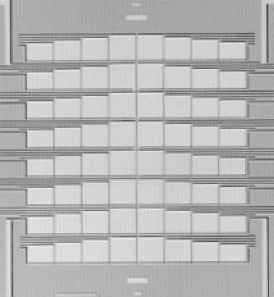
Figure 1: TES Array image. For these observations, we recorded data from the 4 pixels along the midline best illuminated by the focussed fiber. The outermost pixels of the $8\times 8$ configuration are not wired and serve only to mask the substrate.

In operation, the Si substrate is cooled well below the $\sim 100$mK W transition temperature, while the TES sensor is biased in a circuit with a fixed voltage. The resulting current allows the W electron system to self-heat into the middle of the superconducting-normal transition. The TES sensors are thus operating in a regime of strong negative electrothermal feedback (Irwin 1995). A major advance of the present apparatus is the first implementation of a NIST-developed digital feedback system which simultaneously linearizes the SQUID ammeters and functions as the data acquisition system. The digitized feedback signal monitors the TES device current. The data stream is processed through an FPGA with adjustable peak shaping and baseline-restore algorithms. In addition to accurate GPS-stamped arrival times and pulse height measurements for each photon, the system provides a number of quality control indicators including adjustable pile-up flags. Four of the pixels were read with independent digital channels of this new design; these provide the photon set analyzed in this paper. This system is directly scalable to large numbers of read channels and can be modified to allow multiplex reading of several pixels per read channel (Chervenak et al. 1999).

There are two serious challenges in coupling these TES detectors to a typical ground-based astronomical telescope. One is to filter the incident beam so that the large flux of thermal photons (at $\lambda>2\mu$m) from the warm optics does not saturate the TES sensor system, which has a modest maximum count rate. The second challenge is to maximally couple the beam of a large telescope to our present small (effectively 46$\mu$m) detector array. In the system described here we used a focal reducing train of fiber and imaging optics (Figure 2). Given the relatively large plate scale ($232\mu$m/arcsec at the f/17.7 Cassegrain focus of the 2.7m telescope) and best expected image of 1-1.5^′′ FWHM we adopted a 400$\mu$m (1.7 arcsec) entrance aperture and fed the light through a 2:1 reducing taper. This taper, along with the $\sim 25$m run of 200$\mu$m-core fiber to the refrigerator bulkhead, were fabricated from low OH, low impurity (Polymicro FSU) Si/Si step-index fibers, providing both good IR and UV transmission. At the bulkhead of the cryostat, a portable ³He/⁴He dilution refrigerator, an ST-connector vacuum feedthrough passed the light to a $\sim 5$m length of high OH ‘wet’ 200$\mu$m core fiber. The bulk of this fiber was spooled in thermal contact with the 1K stage of the cryostat. In this way the strong OH absorption bands of the wet fiber (Humbach 1996) acted to provide a cold filter with effective blocking beyond 1.7$\mu$m and several strong shorter wavelength absorption bands (e.g. at 0.95$\mu$m). These absorptions correspond to wavelengths of strong atmospheric OH emission. The system thus provided transmission in the astronomically interesting J and H bands as well as reasonable throughput to 400nm where scattering in the fibers began to compromise transmission.

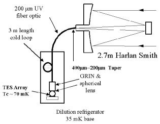
Figure 2: Schematic of TES Spectrophotometer system

To illuminate the sensor array at the cold stage, we collimated the fiber beam with a 1.8mm 1/4 pitch gradient index (GRIN) lens and then focused with a 1.0mm diameter spherical lens to provide the best coupling to the central $2\times 2$-pixel section of the TES array. Despite inevitable focal ratio degradation in the fiber train, the final $\sim f/1$ focus with modest chromatic aberration ensured that we had reasonable coupling into our central 160$\mu$m² of active W TES. We measured the absolute quantum efficiency of the system from the cryostat bulkhead to final recorded photons, including the $\sim 50\%$ absorptivity of the grey tungsten surface, using a calibrated 850nm light source, calibrated attenuators and an absolute power meter. These measurements determined a total 850nm QE of 0.097. This was confirmed by comparison with CCD integrations, using cameras of known QE. The ‘rail’ hit photons contribute an additional 0.01 to the system QE. Inevitably, the fiber train to the telescope incurs additional losses. Unfortunately, these were exacerbated by a defect in the ST couplers of the taper section. As a consequence, the fiber section imposed a factor of $\approx 2.5$ decrease in the peak throughput, relative to the back end of the telescope.

3 Calibration

The energy scale for each pixel was set by interrupting the observations every few hours to take short $\sim 60$s exposures of a calibration lamp passed through a grating monochrometer and fiber fed to the TES array. Typically we integrated with the 1^st order set at $\sim$0.5eV, 1.0eV and 2.0eV. Observations of the order peaks provided a quick calibration of the system energy scale and non-linearity. In addition, to monitor any slow drifts in the energy gain as might occur due to baseline temperature drifts in the dilution refrigerator, a series of calibrated ‘heat pulses’ with a range of energies were introduced to the W $e^{-}$ system on a regular cadence throughout the data exposures. These pulses produce photon-like signals of known arrival time and amplitude interleaved through the data stream. These heat pulses were excised and monitored for any sign of gain drift. In practice, operation was sufficiently stable that no detectable drifts were generally seen in the heat pulse monitor. The monochrometer calibration spectra were used to form the response matrices $R_{k}(E_{i},\epsilon_{j})$ across detector energy bins $\epsilon_{j}$ to the incoming photon energies $E_{i}$ for each pixel $k$.

Figure 3: The estimated total quantum efficiency of our system (fiber+detector) at the back end of the telescope. Atmospheric absorption, telescope inefficiencies and aperture losses give a typical peak effective efficiency (relative to flux at the top of the atmosphere) of $\sim 1$%. For comparison the count spectrum observed from a 2.06eV setting of a grating monochrometer is shown. The low energy events (dashed line) include a rising continuum due to substrate (Si) hits, as well as a thermal IR H-band peak from the warm optics and lamp.

To complete the spectrophotometric calibration, we observed the Bruzual-Persson-Gunn-Stryker spectrophotometric standard BD+30 2344 at low airmass during each observing night of the run. Although convenient for its well calibrated absolute IR-optical-UV spectral energy distributions, at $m_{V}=10.2$ the star had to be observed with substantial de-focus to avoid detector non-linearities at high count rates. We therefore also observed the $m_{V}=14.9$ blue KPNO flux standard PG 0939+262 (Massey et al. 1988) to allow an improved estimate of the system UV response and a check on the point-source total efficiency, including aperture losses. The fiber filter has strong absorption bands whose width is comparable to or smaller than our energy resolution. Also for steep red spectra, the satellite ‘rail hit’ peak at 1.26 times the main peak energy contributes significantly to the count rate. This made it impossible to extract the flux scale by directly dividing the predicted standard star counts by the observed channel counts. Instead the calibration star spectrum was convolved with the response function, the fiber absorption curve measured at high resolution, and the W absorption spectrum to produce model calibrator count spectra. Comparing in the data space, an effective area function varying slowly with energy was fit to model the additional focus and absorption losses compared to stellar fluxes at the top of the atmosphere. Combining these factors, we derive model efficiency functions $E_{k}(\epsilon_{j})$ for each active pixel $k$. After summing these we have a total (detector+telescope+atmosphere) efficiency for the system; this peaks at $\sim 1.2$%. In Figure 3 we correct this efficiency for the estimated atmospheric extinction, telescope inefficiencies and aperture losses to produce the effective response of the system (fiber optics + detector) at the back end of the telescope. For comparison, the energy ranges corresponding to Johnson broad-band colors are indicated. Variation between the calibration sources indicate that the systematic errors in the flux scale are $<10\%$ for the range 1-2.5eV. In the blue, the calibration spectra have lower S/N and larger contribution from the rail hit events, so the systematic errors in the flux scale rise, probably reaching 30% above 3.5eV. Comparison with archival Crab data below support the idea that our flux scale is systematically high by approximately this amount in the U band. Imprecision in the estimates of the telescope and aperture losses also produce uncertainties exceeding 10% in the absolute flux scale.

4 Crab Pulsar Spectrophotometry

We observed a number of compact object sources, both accretion powered binaries and isolated spin-powered pulsars. The relatively bright ($m_{v}\sim 16.6$) Crab pulsar was used to tune and characterize the system performance.

Our GPS-stamped Crab photon arrival times were reduced to the solar system barycenter employing the widely used TEMPO pulsar timing package (from pulsar.princeton.edu/tempo). We used the monthly Crab pulsar radio ephemeris published by Jodrell Bank (Lyne, Pritchard & Roberts 1999) to phase the photon arrival times. The light curves from our four nights of observation are phased within $\sim 10\mu$s; the absolute phase agrees with the predicted infinite frequency pulse arrival time (referenced to the peak of the main pulse) to within $\sim 30\mu$s. This absolute precision is rather better than the nominal $\sim 100\mu$s accuracy of the published monthly ephemeris and is completely adequate for our purposes, allowing a detailed comparison of our phase bin spectra with other (e.g. space-based) data sets. We focus here on a relatively long (3500s) coherent data set taken on February 6, 2000 (MJD 51581) for which the system parameters were stable and the observing efficiency was high. This data set provides much of our total S/N for the Crab pulsar and represents a unique time- and energy-resolved measurement of this well-studied object. A sample optical (1.5eV-3.5eV) light curve is shown for reference in Figure 4.

Figure 4: A sample 1.5eV-3.5eV (3550 - 8250 Å) $10^{3}$-bin light curve from 3500s of TES Crab data. Phase 0 is referenced to the main peak of the radio ephemeris. The upper histogram shows the same data at 100 bins (zero suppressed), magnified to show the baseline variation. Our selected background region is shown (label BG).

There is appreciable structure in our light curve baseline even at pulse minimum. Previous studies also infer magnetospheric emission throughout the pulse period (e.g. Sanwal et al. 1998). Recently Golden, Shearer & Beskin (2000) have argued from MAMA imaging data that the phase interval 0.75-0.825 represents the DC pulse minimum with $\sim 0.4$% of the integrated pulse emission. Our data show significant structure in this region, but given the substantial background in our our 1.7^′′ aperture, we select the phase interval $\phi_{BG}=0.76-0.87$ for our ‘background’ spectrum, recognizing that there will be a small $<1$% magnetospheric contamination; this will be dominated by Poisson fluctuations in nearly all of our extracted spectra.

Figure 5: Phase-averaged TES Crab spectrum (full line with error flags) compared with broad-band colors. Predicted (extincted $\alpha_{\nu}=0.11$; line histogram) and observed (filled dots) count spectra are shown for comparison (Right scale).

In Figure 5 we show the phase-averaged spectrum after background subtraction, convolution through the response matrix and application of the flux calibration solution of §3. To maximize the independence of the spectral bins, we first compute the expected count spectrum of the best-fit simple absorbed power-law model and then derive the Crab fluxes by multiplying the model flux by the ratio of the observed to predicted counts for each channel. This ‘pre-whitening’ avoids spreading fluctuations in the observed count bins between final spectral bins and ensures that sensitivity to errors in the response matrices are of second order. Nonetheless, the derived spectrum represents only one model (the smoothest) that fits the count data. The error bars shown are Poisson only, derived from the independent counts in the energy bins. For comparison, we plot optical/IR phase-averaged broad-band photometry tabulated in Eikenberry et al. (1997). We also show the phase-averaged spectrum fit by Sollerman et al. (2000) to optical/UV data as the solid histogram – this is an $\alpha_{\nu}=0.11$ powerlaw subject to E(B-V)=0.52, R=3.1 interstellar reddening – displayed as a predicted count histogram. This may be compared with the observed spectrum (solid dots). Notice that, in agreement with the IR photometry of Eikenberry et al. (1997), this powerlaw under-predicts the J/H flux.

It is evident that our derived spectrum shows a somewhat steeper (redder) optical spectrum than the Sollerman et al. power-law fit and also lies below the B & U colors of Percival et al. (1993). This supports the suspicion of a systematic over-estimate of our sensitivity function above 2.5eV (possibly due to incomplete modeling of the rail-hit component of the PSF and/or pile-up). The notch in the spectrum at $E_{\gamma}\sim 0.9$eV is also likely an artefact caused by the rapid variation in the system sensitivity at the OH absorption band. Interestingly, we find that our $E\geq 1$eV spectrum is however very well modeled by an extincted $\alpha=-0.2$ power law, which is actually the same spectrum found originally by Oke (1969). The true spectral index is evidently quite sensitive to the reddening parameters and energy range chosen and, indeed, the optical/UV spectrum of Sollerman et al. shows appreciable curvature. However, given the mismatch with the broad-band photometry in the blue, slight flux calibration systematics are the likely culprit.

We can, of course, study spectral variations in the Crab by assuming that the phase-averaged spectrum is smooth and using our observed total pulsar spectrum as the flux calibrator. This differential measurement allows a much improved removal of small scale variations in the sensitivity function and provides robust detection of any spectral phase variations. Figure 6 shows a selection of phase bin spectra, referenced to the total (phase-averaged) spectrum. There are evidently subtle but continuous variations in the broad-band spectral index and a distinct change in the behavior in the near-IR band (see, for example the break at $\gtrsim 1$eV in the leading edge of the main pulse, spectrum 1). The spectra show little fine structure except at the strong fiber absorption bands. Smooth continuum variations dominate, as expected for a broad-band emission process such as optical synchrotron. Errors are computed by propagating Poisson fluctuations in both the background subtracted spectra and the reference (phase-averaged) spectrum.

Figure 6: Phase bin count spectra. The log of the photon flux is plotted against log($E_{\gamma}$) for several phase bins from the 13 contiguous bins indicated in the panel to the right.

We can measure these smooth variations in smaller $\phi$ bins by fitting. Figure 7 shows a double power-law fit with a fixed break at 1.3eV. To obtain these spectral indices, we correct by a mean (phase-averaged) powerlaw. In view of the calibration uncertainties above, we have chosen to reference the spectra using a phase-averaged index of $\alpha=-0.1$. The spectral index fit errors are derived from the Poisson spectral bin errors above.

Figure 7: Spectral index phase variations. Fits to optical (triangles, Upper panel) and near-IR (open circles, Lower panel) bands are shown. Note the rapid, anti-correlated variation in the main peak, indicating a varying spectral break. For comparison, an optical light curve and X-ray RXTE (Pravdo, Angelini & Harding 1997) phase-resolved spectral indices are shown in the lower panel.

The data show a rapid sweep in the spectral index, especially in the main peak. An optical light curve and peak phase marks are provided for reference. At the leading edge of the main peak the IR index does not reverse, but the spectrum becomes increasingly blue. This indicates strong break or depression of the IR at the leading edge of the main pulse. This is the origin of the IR variation in the leading pulse half-width noted by Eikenberry, et al. (1997). While the phase bins and error flags are large in the bridge between the pulses, the optical and IR indices also differ strongly in this region, with a steep red IR spectrum passing to a much harder component in the blue. This increase of the bridge flux at high energies is in accord with the strengthening of the bridge emission in the X-ray and $\gamma$-ray bands.

Phase-dependent spectral indices were first noticed in the Crab in the X-ray band (Pravdo & Serlemitsos 1981). The reference Rossi X-ray Timing Explorer (RXTE) data above and more extensive BeppoSAX opservations reported by Massaro et al. (2001) show rapid variation in the hard X-ray power-law spectrum, especially near the first peak. The phase coincidence of the optical/IR variations imply a common origin, but there is evidently no simple relation between the indices in the two band. At higher $\gamma$-ray energies limited count rates do not allow the fine phase bins used in the X-ray analysis, but a correlated spectral variation is seen across the Crab pulse profile (Fierro 1995).

In the optical, many authors starting with Muncaster & Cocke (1972) have used used time-resolved color photometry to suggest that the bridge region is bluer than the pulses. This is seen most clearly in the largely unpublished UBVR observations reported in Sanwal et al. (1998). Recently, Golden et al. (2000) have reported a reddening in the bridge region, based on UBV photometry, but this does not accord with other recent measurements. Note that with the exception of the Sanwal et al. (1998) data, limited count statistics forced all observations to use very coarse phase bins, typically summing over the entire pulse or interpulse. The $\alpha$ sweeps we see are located largely within these components; this is a likely explanation for the non-detection of spectral variation in several studies (e.g. Carraminana, Cadez & Zwitter 2000, Perryman et al. 1999). Thus the optical $\alpha$ variations through the pulses are seen here clearly for the first time.

The simultaneous IR measurements of this data set also provide a new window on the pulsar physics, given the rapid variation in the spectral break below $\sim 1$eV. Simultaneous optical/IR spectra were first reported in Romani et al. (1999). Recent simultaneous dual band (V & H) light curves have also been reported by Moon et al. (2001), but the low efficiency and limited S/N of these test data likely preclude measurement of the subtle spectral variations. Although some interesting indications of spectral variations can clearly be seen in the broad-band (non-simultaneous) IR photometry of Eikenberry et al. (1997), the data reported above are the first to show these fine-resolution spectral variations extending into the infrared. While the variations are highly significant, longer integrations with better S/N are certainly desirable. Nonetheless, these data already provide some constraints on the radiation processes, which we describe briefly in §7.

5 Crab Photon Statistics

At our roughly kilohertz count rates, we detected $\sim$25 photons in each main pulse, giving us substantial sensitivity to photon correlations. In the radio most pulsars exhibit a Gaussian or log-normal distribution of pulse intensities. The Crab, however, also produces occasional radio pulses with up to $\sim 10^{3}\times$ the mean pulse energy. These ’Giant pulses’ are short duration bursts of flux, appearing randomly in narrow windows of pulsar phase. Lundgren et al. (1995) have searched for and placed limits on any correlation between giant radio pulses and $\gamma$-ray emission, while Patt et al. (1999) have found that no giant pulses are present in the X-ray band. Percival et al. (1993) have also found no non-Poisson pulse-to-pulse variations in the optical flux of the individual pulse components. Lacking simultaneous radio data, we examined our data for any short-time scale photon correlations.

We searched for non-Poisson photon distributions by predicting the expected counts in a range of lag bins following each observed photon. Because each detector has a small $\sim 10\mu$s dead time associated with the recovery from a photon pulse, we searched the cross-correlations between our pixels, allowing us to extend the analysis to microsecond times. To test the null Poisson hypothesis, we need an accurate estimate of the expected count rate in the face of the varying pulsed emission and background in our aperture. This was obtained by forming a 100-bin light curve for each second of data and fitting the counts to a background and pulsed flux amplitude. For each photon arriving during this second, we used the two fit amplitudes to predict the photon arrival rate in the other three detectors on a range of timescales. The model flux in each lag bin was determined by an integration through the appropriate phases of a high-resolution ($10^{3}$bin Figure 4) light curve from all the data in a selected energy range, scaled to the instantaneous detected flux. The observed counts can be compared to the Poisson expectation for photons of a given energy range on various timescales and over various windows of pulsar phase. No strong energy dependency was noted, so we show the statistics of the full low background 1-4eV energy range.

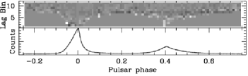
Figure 8: Ratio of average rate to Poisson rate for $E_{\gamma}\geq 1$eV. The grey scale image shows the ratio in independent lag bins, spaced as even octaves (vertically), vs. pulse phase (horizontally). Light shows high correlation and dark shows sub-Poisson counts. Bins with $<25$ counts are set to 1.

Figure 8 shows as a gray intensity scale the observed count rate in units of the Poisson predicted rate in 100 bins of pulsar phase. The vertical axis of the grey scale shows correlation bins covering time lags $\delta\tau=t_{samp}(2^{N}-2^{N-1})$, where $t_{samp}=0.31\mu$s. $N$ runs from 1 to 11 ($\tau=0.3\mu$s to $635\mu$s) in the gray scale plot shown. The lag bins are thus completely statistically independent. A significant correlation (or anti-correlation) on short time scales would be expected to show as a coherent bright (or dark) region at the appropriate phase, fading to grey in longer timescales. The data show fluctuations in the individual amplitudes when the counts are low. There is a $\sim 10-15$% enhancement on timescales $\tau\sim 5-10\mu$s leading the first peak by $\sim 1$ms; this is of $\sim 3\sigma$ significance. There is also a $\sim 30$% enhancement at $\tau\leq 3\mu$s leading the second peak, but this is only $\sim 2\sigma$ in the most significant lag bin. A few percent decrement at lag $N=7$ appears correlated with noise in the 33$\mu$s bins in the fine template. All other significant features are smaller than 1%. We conclude that our photon arrival times are consistent with Poisson and that there is no evidence for strong correlations on short timescales, such as giant pulses, at optical energies.

6 Crab Spectrophotopolarimetry

Ultimately, complete exploitation of astronomical fluxes requires time-resolved spectrophotopolarimetry. The strong, rapidly varying polarization of the Crab pulsar makes it an attractive test target. Phase resolved polarimetry has been presented in the optical (Smith et al. 1988) and the near UV (Smith et al. 1996), which give a basis for comparison. The double position-angle sweep reported in these papers has been shown to be a good quantitative match to a relativistic outer magnetosphere version of the rotating vector model by Romani and Yadigaroglu (1995). In this model emission from a range of altitudes forms caustics in photon arrival phase that define the pulses. Further, a combination of two distinct emitting regions can contribute to the interpulse phases. If the radiating populations (and hence spectral indices and breaks) differ between these regions we would expect energy dependence of the polarization fraction.

As a test, we observed the Crab pulsar on February 7, 2000 (MJD 51582) with a simple polaroid filter placed before the focal plane. We integrated at two full cycles of position angle with the following exposures: $0^{\circ}$ (1370s,630s), $45^{\circ}$ (520s,690s), $90^{\circ}$ (740s,620s), $135^{\circ}$ (960s,680s) with angles referenced to the equatorial coordinate system. Of course, varying background and varying aperture losses between the exposures mean that the light curves must be renormalized before forming $q=(I_{0}-I_{90})/(I_{0}+I_{90})$ and $u=(I_{45}-I_{135})/(I_{45}+I_{135})$. To subtract the substantially polarized nebular emission in our aperture, we employed our usual background phase window (0.76-0.87), following the prescription in (Smith et al. 1996). While residual pulsar emission at these phases may be highly polarized (Smith et al. 1988), the amplitude is small enough that its contamination of the peaks and bridge region should be smaller than our statistical errors. An examination of the Smith et al. (1988) data (kindly supplied in digital form by F.G. Smith) showed a polarization minimum during the bright first pulse in the region $\phi=$0.005-0.025, consistent with 0, within the error bars. This provides a convenient exposure monitor based on the pulsed emission itself. These data were taken in a broad optical band with the ‘RGO people’s photometer’; we synthesized this band in our data, selecting the appropriate energy bins and using the polarization minimum flux as a monitor of the total Crab exposure at each polarization position angle.

Figure 9: Test Crab Spectropolarimetry in three optical bands. Two pulse periods are shown for clarity. Above: Position angle. An optical light curve is included for phase reference. Below: Linear polarization fraction.

In Figure 9, we show the resulting polarization fraction $p=(q^{2}+u^{2})^{1/2}$ corrected for the wavelength dependent polarization efficiency of the filter (measured using monochrometer light passed through crossed filters). We also corrected for the bias due to non-normal statistics at small polarization, with the observed polarization $p_{0}$ corrected to $p=p_{0}[1-(\sigma/p_{0})^{2}]^{1/2}$. In the upper panel we show the polarization position angle $\theta=1/2\times{\rm Arctan}(u/q)$. The error flags shown are the propagated Poisson errors. Differences between the two sets of position angle data were within the statistical errors, so these were summed in the polarization amplitude and sweep shown. Limited statistics restricted us to 18 phase bins through the pulse, so fine structure is likely not fully resolved.

The overall polarization behavior follows that measured in previous optical/UV experiments quite closely. We show the optical data divided into three energy bands. The rapid decrease in polarization and strong position angle sweep of the first pulse appear quite energy independent. There are small differences in the polarization and position angle of the bridge and second pulse, but these are of marginal significance. Given that the phase variations in the spectral index and break are strongest below 1.5eV (§4) we might expect the strongest spectral effects in the near-IR. Indeed, our near IR data do appear to show significantly different polarization properties. Unfortunately, the increased IR background and difficulty in calibrating the rapidly varying IR polarization response of the filter preclude a quantitative comparison with the optical data in the present experiment. Serious phase-resolved spectropolarimetry will require imaging solutions for local background subtraction; as part of our next-generation imaging system (see below), we plan to install Wollaston prisms for imaging spectrophotopolarimetry over reduced fields.

7 Spectral Variations and Conclusions

The phase variations through the Crab profile described above clearly provide new tests of the physics of the optical/IR radiation. The polarized IR through hard X-ray non-thermal emission from the Crab is generally held to be synchrotron radiation from a population of $e^{\pm}$ propagating and cooling in the outer magnetosphere (e.g. Lyne and Smith 1990 and references therein; Romani 1996; Wang, Ruderman & Halpern 1998). The broad-band phase-averaged SED is smooth, with $\alpha$ varying from $-0.7$ (hard X-rays) through $-0.5$ (soft X-rays) to $\sim 0$ at optical frequencies. There is evidently a peak in the near-IR and then the spectrum drops off dramatically at lower energies (Middleditch, Pennypacker & Burns 1983), although this important result definitely requires confirmation.

Recently, Crusius-Waetzel et al. (2001) have provided a synchrotron interpretation that provides a plausible explanation of the soft-X-ray through IR phase averaged SED in terms of a single $N\propto E_{e^{\pm}}^{-s}$ population (presumably produced through an $e^{\pm}$ pair cascade in the outer magnetosphere) with $s=2$. In the X-ray band, the emission is assumed to be classical relativistic synchrotron radiation with $F_{E}\propto E^{-(s-1)/2}$; this gives the observed $\alpha\approx-0.5$ spectrum observed for the powerlaw X-ray emission of the Crab and other young pulsars. However, Crusius-Waetzel et al. additionally argue that the $e^{\pm}$ population should have a component with very low pitch angle $\Psi\ll 1/\gamma$, for which the synchrotron emission formulae give $F_{E}\propto E^{2-s}$, when averaged over the radiating beam. For the Crab, they infer $\gamma\sim 10^{2}-10^{3}$ and $\Psi<10^{-3}$, and connect the $\alpha\approx 0$ spectrum with that seen in the optical. Finally, they suggest that below $1$eV the particles dominating the emission spectrum have even lower $\gamma$, so that the observed pulse width $\Delta\phi\sim 0.01$ samples only a subset of the $1/\gamma$ radiation cone and argue that this leads to a $F_{E}\propto E^{4-s}$ spectrum. This index is taken to be, at least in part, an explanation of the steep rise in the mid-IR.

Figure 10: Low pitch-angle prediction for the optical spectral index variation (full line) compared with optical and IR TES data.

If we take the X-ray spectral index to be a local measurement of the electron powerlaw $s$ then this picture predicts the correlated optical spectrum in the low pitch angle limit. In Figure 10, we show the TES data compared with this prediction, based on the 0.1-4.0 keV data of Massaro et al. (2001). Clearly this phase bin application of the low pitch-angle picture is not adequate: while the index and trend for the second pulse are reasonably well predicted, the spectra of the bridge region and, especially, the first pulse show no match to the extrapolations of soft X-ray data. When one considers that the spectral index in all phase bins steepen into the hard X-rays, then one must conclude that a simple application of powerlaw synchrotron emission, even with a phase-varying $s$, is not adequate.

One factor likely important in a more complete model is the inclusion of the local beaming of the radiation cones along the emission surface. Given the sharp pulses and the observation at a single line-of-sight, the radiation must differ from the emission-cone averaged synchrotron expressions above. Models including these effects are sensitive to the detailed geometry. As an example, consider the strong IR break at the leading edge of the main pulse. In the outer magnetosphere caustic picture of the pulse formation, the leading edge of the main pulse arises from emission propagating along the radiating surface for the longest distance. Hence, one would expect this to be the region first showing self-absorption suppression. While the overall IR suppression of the main peak reported by Penny (1982) suggestive of uniform self-absorption is not seen in our data, the observed leading edge suppression and steepening may be a more restricted instance of self-absorption. Polarization measurements extended into the IR will be a good discriminant between absorption effects and emission breaks, as a restricted sampling of the synchrotron emission cone leads to polarization signatures varying significantly in accord with the spectral breaks.

We are developing a focal plane camera based on TES detector arrays, with the potential for time resolved imaging spectral polarimetry. As the data of Golden et al. (2000) and Perryman et al. (1999) show, the absolute photometry and background subtraction of such true imaging measurements can provide much improved isolation of faint pulsar phenomena. With the clean monoenergetic energy PSF of a ‘masked’ TES array, improved system QE and improved energy resolution, observations of the Crab (and other fainter pulsars) should allow a detailed examination of the phase-resolved phenomena discovered in the exploratory measurements reported here.

References

- (1) Cabrera, B., et al. 1998, Appl. Phys. Let., 73, 735.
- (2) Carraminana, A., Cadez, A. Zwitter, T. 2000, ApJ, 542, 947.
- (3) Chervenak, J.A., et al. 1999, Appl. Phys. Lett., 74, 4043.
- (4) Crusius-Wätzel, A.R, Kunzl, T. & Lesch, H. 2001, ApJ, 546, 401
- (5) Eikenberry, S.S., et al. 1997, ApJ, 476, 281.
- (6) Fierro, J.M. 1995, PhD Thesis, Stanford University.
- (7) Golden, A., Shearer, A. & Beskin, G.M. 2000, ApJ, 535, 373.
- (8) Golden, A., et al. 2000, AA, 363, 617.
- (9) Humbach, O., et al. 1996, Journal of Non-Crystaline Solids, 203, 19.
- (10) Irwin, K.D. 1995, Appl. Phys. Lett., 66, 1998.
- (11) Lundgren, S.C. et al. 1995 ApJ, 453, 433.
- (12) Lyne, A.G., Pritchard, R.S. and Roberts, M.E. 1999, (http://www.jb.man.ac.uk/pulsar/crab.html)
- (13) Lyne, A.G. & Smith, F.G. 1998, Pulsar Astronomy (Cambridge:Cambridge).
- (14) Massaro, E., Cusumano, G., Litterio, M. & Mineo, T. 2001, AA, ,
- (15) Massey, P., Strobel, K., Barnes, J.V & Anderson, E. 1988, ApJ, 328, 315.
- (16) Middleditch, J., Pennypacker, C. & Burns, M.S. 1983, ApJ, 273, 261.
- (17) Miller, A.J., et al. 2000, NIMPA, 444, 445.
- (18) Moon, D.-S., Pirger, B.E. & Eikenberry, S. 2001, PASP, 113, 646
- (19) Muncaster, G.W. & Cocke, W.J. 1972, ApJ, 178, L13
- (20) Oke, J.B. 1969, ApJ, 156, L49
- (21) Patt, B.L., Ulmer, M.P., Zhang, W., Cordes, J.M. & Arzoumanian, A. 1999, ApJ, 522, 440.
- (22) Penny, A.J. 1982, MNRaS, 198, 773
- (23) Percival, J.W. et al. 1993, ApJ, 407, 276
- (24) Perryman, M.A.C., Foden, C.L., & Peacock, A. 1993, Nucl. Instr. Meth., A325, 319.
- (25) Perryman, M.A.C., Favata, F., Peacock, A., Rando, N. & Taylor, B.G. 1999, AA, 346, L30.
- (26) Pravdo, S.H. & Serlemitsos, P.J. 1981, ApJ, 246, 484.
- (27) Pravdo, S.H. Angellini, L. & Harding, A.k. 1997, ApJ, 491, 808.
- (28) Romani, R.W. 1996, ApJ, 470, 469.
- (29) Romani, R.W., et al. 1999, ApJ, 521, L153.
- (30) Romani, R.W. & Yadigaroglu, I.-A. 1995, ApJ, 438, 314
- (31) Sanwal, D., Robinson, E.L. & Stiening, R.F. 1998, BAAS, 30, 1420.
- (32) Smith, F.G., Jones, D.H.P., Dick, J.S.B. & Pike, C.D. 1988, MNRaS, 233, 305.
- (33) Smith, F.G., et al. 1996, MNRaS, 282, 1354
- (34) Sollerman, J. et al. 2000, ApJ, 537, 861.
- (35) Wang, F.Y.-H., Ruderman, M. & Halpern, J.P. 1998, ApJ, 498, 373
- (36) Wollman, D.A. et al. 2000, NIMPA, 444, 145.
- (37)
- (38)
- (39)