The proximity effect in a close group of QSOs

Abstract

We present an analysis of the proximity effect in a sample of ten $2\,$Å resolution QSO spectra of the Ly$\alpha$ forest at $\langle z\rangle=2.9$. Rather than investigating variations in the number density of individual absorption lines we employ a novel technique that is based on the statistics of the transmitted flux itself. We confirm the existence of the proximity effect at the $>99$ per cent confidence level. We derive a value for the mean intensity of the extragalactic background radiation at the Lyman limit of $J=3.5^{+3.5}_{-1.3}\times 10^{-22}$ ergs s^-1 cm^-2 Hz^-1 sr^-1. This value assumes that QSO redshifts measured from high ionization lines differ from the true systemic redshifts by $\Delta v\approx 800$ km s^-1. We find evidence at a level of $2.6\sigma$ that the significance of the proximity effect is correlated with QSO Lyman limit luminosity. Allowing for known QSO variability the significance of the correlation reduces to $2.1\sigma$.

The QSOs form a close group on the sky and the sample is thus well suited for an investigation of the foreground proximity effect, where the Ly$\alpha$ forest of a background QSO is influenced by the UV radiation from a nearby foreground QSO. From the complete sample we find no evidence for the existence of this effect, implying either that $J>20\times 10^{-22}$ ergs s^-1 cm^-2 Hz^-1 sr^-1 or that QSOs emit at least a factor of $1.4$ less ionizing radiation in the plane of the sky than along the line of sight to Earth. We do however find one counter-example. Our sample includes the fortunate constellation of a foreground QSO surrounded by four nearby background QSOs. These four spectra all show underdense absorption within $\pm 3000$ km s^-1 of the redshift of the foreground QSO.

1 Introduction

The study of many physical processes at high redshift requires knowledge of the intensity of the UV background radiation, $J$. For example, it is thought that the Ly$\alpha$ forest in QSO absorption spectra is caused by highly photo-ionized gas and thus an estimate of the total mass content of the intergalactic medium (IGM) depends on $J$ [Rauch et al. (1997), Weinberg et al. (1997)]. It is also one of the parameters that define the environment in which galaxies form (e.g. [Susa & Umemura (2000)]), and its value and evolution provide important constraints on the objects believed to be the origin of the background (e.g. [Bechtold et al. (1987)]; [Haardt & Madau (1996)]; [Fardal et al. (1998)]). At high redshift, the background is often measured from the proximity effect, i.e. the observed underdensity of Ly$\alpha$ forest absorption lines in the vicinity of background QSOs.

Nearly $20$ years ago ?) first noted that the mean density of Ly$\alpha$ absorption lines seemed to increase with redshift when comparing the spectra of several different QSOs and yet decrease along individual lines of sight. ?) confirmed this ‘inverse effect’, established that it was confined to the vicinity of the QSO (‘proximity effect’) and offered two possible explanations: i) the absorbers near a QSO may be too small to fully cover the continuum emitting region or ii) absorbers in the vicinity of a QSO may be more highly ionized than elsewhere due to the QSO’s UV radiation.

In a seminal paper ?) (hereafter BDO) developed a quantitative ionization model and, for the first time, measured $J$ from the observed underdense absorption near $19$ QSOs and their observed luminosities. In the most comprehensive intermediate resolution study to date ?) analysed a sample of $74$ spectra. Like ?), they divided their sample into low and high-luminosity subsamples and found that the relative deficit of absorption lines within $1.5~{}h^{-1}_{75}$ Mpc of the background QSOs was more significant in the latter.

?) studied the proximity effect at high spectral resolution. In their thorough analysis of $11$ spectra they gave a detailed account of the various statistical and systematic errors and biases involved in the measurement of $J$ from the proximity effect. Like previous authors they found no evidence to suggest that the background intensity evolved with redshift.

We summarize these and other measurements of $J$ in Fig. 2. It is worth noting that not all the points in this plot are independent of one another. There are large overlaps in the data used. For example, Q0014+813 is included in eight of these studies. In addition, all except one of these measurements are based on ‘line counting’, i.e. the statistics of individual absorption lines. Only ?) considered the integrated absorption in $100\,$Å bins. ?) obtained a rough estimate of $J$ from $W^{-1}$ correlations (where $W$ is the rest equivalent width) and ?) used a basic flux statistics approach to investigate the foreground proximity effect. Thus no alternative methods seem to have been explored in great detail.

Figure 2: Summary of previous proximity effect measurements of the mean background Lyman limit intensity, $J$, in units of $10^{-21}$ ergs s^-1 cm^-2 Hz^-1 sr^-1. Solid and open symbols represent measurements from intermediate and high resolution data respectively. Estimates from the background (foreground) proximity effect are shown as circles (triangles), those that include both are shown as squares. Error bars are $1\sigma$. The dashed line marks the value of $J$ at $z=2.5$–$3$ computed by Haardt & Madau (1996) for a background dominated by the observed QSO population and for a $q_{0}=0.1$ cosmology. The top panel shows the redshift intervals covered by the various studies.

Most authors have found good agreement between their data and the ionization model of BDO and alternative explanations for the proximity effect have not received much observational support. The sizes of Ly$\alpha$ absorbers inferred from observations of close QSO pairs (e.g. [Dinshaw et al. (1998)] and references therein) seem to rule out the possibility that the absorbers are too small to completely cover the background QSO. In addition, ?) found no difference between the $W$ distribution of lines near QSOs and that of lines far from QSOs. They also eliminated a broken power law for the redshift distribution of lines as a possible cause for the proximity effect.

Thus increased ionization due to the extra UV flux from the QSO seems to remain as the only credible explanation for the proximity effect. However, it implies two observable effects:

1. The proximity effect should correlate with QSO luminosity. More luminous QSOs should deplete larger regions more thoroughly than less luminous ones. BDO claimed that this effect was present in their data and that it was consistent with the expectations from their ionization model. ?) and ?) also found a weak correlation. ?) on the other hand found no evidence for a correlation at all but nevertheless concluded on the basis of simulations that this was consistent with the ionization model. ?) could not identify a correlation either.

2. In addition to the ‘classical’ background proximity effect there should be a foreground proximity effect where the absorbing gas along the line of sight to a background QSO is depleted by the UV radiation of a close-by foreground QSO. Studying a triplet of QSOs separated by $2$ to $3$ arcmin ?) found no evidence for the existence of the foreground proximity effect. ?) added another spectrum to this triplet and confirmed the negative result. ?) observed a $\sim 10$ Mpc void in the spectrum of Q0302–003 with a foreground QSO separated from its line of sight by $17$ arcmin. However, the foreground QSO was displaced from the void by $\sim 3600$ km s^-1, implying either that the QSO radiates anisotropically or that it turned on on a time-scale comparable to the light travel time from the QSO to the void. ?) studied three QSO pairs separated by $3.8$ to $12.6$ arcmin but they were unable to reject the non-existence of the effect by more than $\sim 1\,\sigma$. Finally, ?) reported a $\sim 7$ Mpc void in the spectrum of Tol 1038–2712 with a foreground QSO at the redshift of the void and separated by $17.9$ arcmin. Like [Dobrzycki & Bechtold (1991)] he showed that it was unlikely that the void was a chance occurrence. Thus there currently exists only a single example where an underdensity of absorption lines in the spectrum of a background QSO can be explained by the presence of a foreground QSO without making extra assumptions.

The main goals of this paper are to introduce a new method to analyse QSO spectra for the proximity effect and to address the two problems described above. The data used in this investigation are described in Section 2. They consist of the spectra of a close group of $10$ QSOs which have not been included in any previous studies. Thus the analysis presented here is independent from others in the sense that it uses both a different method as well as different data. In Section 4 we measure $J$ from the classical proximity effect and demonstrate its correlation with QSO luminosity. In Section 5 we turn to the foreground proximity effect. Finally, we consider a range of uncertainties in Section 6 and discuss our results in Section 7.

Unless explicitly stated otherwise we use $q_{0}=0.5$, $\Lambda=0$ and $H_{0}=100\,h$ km s^-1 Mpc^-1 throughout this paper.

2 The data

?) performed a large C iv survey in the South Galactic Pole region. Here, we use that subset of the data which has reasonable coverage of the Ly$\alpha$ forest (10 spectra). The instrumental resolution is $\sim 2\,$Å and the signal-to-noise ratio per pixel reaches up to 40 per $1\,$Å pixel. The observations and the reduction process are described in detail by ?).

Figure 4: Distribution of QSOs in the sky. The field is centered on $\alpha=00^{{\rm h}}42^{{\rm m}}10^{{\rm s}}$ and $\delta=-26\hbox{${}^{\circ}$}40\hbox{${}^{\prime}$}$ (B1950). Solid stars mark the positions of the QSOs whose spectra are analysed in this paper. Empty stars mark the positions of additional foreground QSOs in the field. Emission redshifts are indicated.

Table 2: QSOs.

Object	$z_{\rm Q}$	$m_{B}^{a}$	$\alpha$	$L_{\nu}(912)^{b}$	Refs.
Q0041–2607	$2.505$	$17.23$	$-0.60$	$15.01$	1, 2
Q0041–2638	$3.053$	$18.35$	$-0.53$	$12.17$	1, 2
Q0041–2658	$2.457$	$18.70$	$-0.88$	$2.34$	1, 2
Q0041–2707	$2.786$	$18.03$		$10.14$	1, 2
Q0042–2627	$3.289$	$18.55$		$13.29$	1, 2
Q0042–2639	$2.98$	$20.05$	$-0.09$	$4.59$	3
Q0042–2656	$3.33$	$19.55$	$-0.80$	$4.11$	3
Q0042–2657	$2.898$	$18.78$		$5.88$	1, 2
Q0042–2714	$2.36$	$19.88$		$1.09$	4, 2, 5
Q0043–2633	$3.44$	$19.61$	$-0.77$	$5.01$	3
Additional foreground QSOs:
Q0040–2606	$2.47$	$19.48$		$1.80$	4, 2
Q0041–2622	$2.18$	$19.28$		$1.69$	4, 2, 5
Q0042–2642	$2.81$	$20.60$	$-1.40$	$0.28$	3
Q0043–2555	$3.31$	$20.53$	$-0.89$	$1.43$	3
Q0043–2606	$3.11$	$20.37$	$-0.96$	$1.07$	3
Q0044–2628	$2.47$	$19.28$		$2.18$	4, 2, 5
Q0044–2721	$3.16$	$20.17$	$-0.45$	$3.05$	3

^aThe typical error on $m_{B}$ is $0.15$.

^bIn units of $10^{30}\>h^{-2}$ ergs s^-1 Hz^-1.

References: (1) Redshifts and $B_{J}$ magnitudes from ?). Where given, continuum slopes were measured from low-resolution spectra kindly provided by Paul Francis.

(2) We converted from $B_{J}$ to Johnson $B$ using the colour equation of ?) and assuming $(B-V)=0.3$.

(3) ?). Conversion to $B$ magnitudes using the colour equation of ?).

(4) ?).

(5) Redshifts from ?).

A search of the literature revealed seven additional QSOs in this field and in the appropriate redshift range. These will be considered as potential foreground ionizing sources. The angular separations range from $6.1$ to $95.8$ arcmin and the emission redshifts range from $2.18$ to $3.44$. The distribution of all of these QSOs in the sky is shown in Fig. 4.

Since absolute spectrophotometry was not available for any of these QSOs we had to estimate continuum flux densities from observed $B$-band magnitudes. Assuming a power law continuum $f_{\nu}\propto\nu^{\alpha}$ the observed flux density $f_{\nu}$ at observed wavelength $\lambda$ is given by

$$f_{\nu}(\lambda)=\left[\frac{\lambda_{X}}{\lambda(1+z_{\rm Q})^{-1}}\right]^{\alpha}(1+z_{\rm Q})\>10^{-0.4(m_{X}-k_{X})}f_{\nu X}(0)$$ (1)

where $\lambda_{X}$, $m_{X}$, $k_{X}$ and $f_{\nu X}(0)$ are the central wavelength, observed magnitude, $K$-correction and 0-magnitude flux [Allen (1991)] of the $X$-band respectively. For $X=V$ and $\alpha=-0.6$ this equation gives a flux $1.6$ times higher than [Tytler (1987)]’s (?) empirical formula. However, note that [Tytler (1987)] used the $K$-corrections of ?) whereas we use the $K$-corrections given by ?) because they extend beyond $z=2.5$. For some QSOs continuum slopes were not available. In these cases we used $\alpha=-0.6$ which is similar to the value of $-0.5$ given by ?).

We correct the above flux value for Galactic extinction by applying a correction factor $10^{0.4A(\lambda)}$ where

$$A(\lambda)=R_{V}\>E(B-V)\>\frac{A(\lambda)}{A(V)}.$$ (2)

We use $R_{V}=A(V)/E(B-V)=3.1$ which is the average value for the diffuse interstellar medium [Clayton & Cardelli (1988)]. The variation of the extinction with wavelength relative to that at $V$, $A(\lambda)/A(V)$, is given by ?) (optical) and ?) (UV). We take $E(B-V)$ for each QSO from the dust map of ?). This procedure is equivalent to first correcting $m_{B}$ for Galactic extinction and then applying a correction to $\alpha$ due to the wavelength dependence of the extinction.

?) first pointed out that QSO redshifts measured from high ionization emission lines like Ly$\alpha$ or C iv are systematically lower than redshifts measured from lower ionization lines like Mg ii or the Balmer series which are thought to indicate the systemic redshifts. When estimating $J$ from the classical proximity effect using QSO redshifts derived from high ionization lines, the result will be too high because the lower QSO redshift implies a higher QSO flux at a given cloud and therefore (for the same observed effect) a higher background. ?) showed that a velocity shift of $\sim 1500$ km s^-1 lowered the value of $J$ from $\log J=-20.75$ to $-21.30$ in [Lu et al. (1991)]’s (?) data.

The redshifts of the QSOs considered in this paper were all determined from high ionization lines. However, since there is considerable disagreement in the literature over the values of the line shifts and possible correlations with QSO luminosity and/or emission line properties (e.g. [Tytler & Fan (1992)] and references therein), it is difficult to reliably correct for this effect. We shall therefore resort to determining $J$ as a function of line shift in Section 4.2.

In Table 2 we list all the QSOs considered as well as their redshifts, $B$-band magnitudes, continuum slopes and Lyman limit luminosities calculated from equations (1) and (11).

3 Analysis

3.1 Method

Essentially, we use the method of ?) (hereafter LWC) to look for regions of underdense absorption (i.e. ‘voids’) in Ly$\alpha$ forest spectra near the positions of suspected sources of ionizing radiation. These sources may be the background QSOs themselves or foreground sources near the line of sight to the background QSOs. The technique does not rely on investigating variations of the number density of individual absorption lines but rather uses the statistics of the transmitted flux directly. Thus it elegantly sidesteps all problems related to the incompleteness of lines due to limited spectral resolution and signal-to-noise, $W$-limited versus $N$-limited samples [Chernomordik & Ozernoy (1993), Srianand & Khare (1996)] and Malmquist bias [Cooke et al. (1997)]. ?) have previously employed a somewhat more rudimentary version of our method to investigate the foreground proximity effect. Flux statistics have also been used in other contexts by ?), ?), ?), ?), ?), ?), ?), ?), ?) and ?).

In order to identify large-scale regions of underdense absorption we convolve a spectrum with a smoothing function in order to filter out the high-frequency ‘noise’ of individual absorption lines. A large-scale feature will be enhanced most by this convolution if the scale of the smoothing function, $\sigma_{\rm s}$, is similar to the scale of the feature. Since we do not know the scale of any possible features a priori we simply smooth the spectrum on all possible scales, from 1 pixel where the data remain unchanged to the largest possible scale where the data are compressed into a single number akin to $1-D_{A}$ [Oke & Korycansky (1982)]. When plotted in the wavelength–smoothing scale plane this procedure results in the ‘transmission triangle’ of the spectrum which we denote by $G(\lambda,\sigma_{\rm s})$ for the case of a Gaussian smoothing function and by $T(\lambda,\sigma_{\rm s})$ for the case of a top-hat smoothing function (Section 3.4).

We then compare the observed transmission to the expected mean transmission calculated on the basis of the simple null-hypothesis that any Ly$\alpha$ forest spectrum can be described as a collection of absorption lines whose parameters are uncorrelated. We also calculate the expected variance of the transmission in order to assess the statistical significance of any fluctuations of the observed transmission around the expected mean.

3.2 Basic absorption model

LCW considered a (normalized) Ly$\alpha$ forest spectrum as a stochastic process where each point in the spectrum is a random variable, e^-τ, drawn from the transmission probability density function. They calculated the mean and variance of this function on the basis of the above null-hypothesis. Including instrumental effects in their calculation they then used these results to derive the mean and variance of $G$,

$$\langle G\rangle(\lambda,\sigma_{\rm s})=\exp\left[-B\left(\frac{\lambda}{\lambda_{\alpha}}\right)^{\gamma+1}\right]$$ (3)

and

$$\sigma_{G}^{2}(\lambda,\sigma_{\rm s})=\frac{\sigma_{n}^{2}(\lambda)}{2\sqrt{\pi}\;\sigma_{\rm s}/ps}+\frac{\sigma_{{\rm e}^{-\tau}}^{2}(\lambda)}{\sqrt{2\frac{\sigma_{\rm s}^{2}+\sigma_{\rm LSF}^{2}}{q^{2}(\lambda)}+1}},$$ (4)

where

$$\sigma_{{\rm e}^{-\tau}}^{2}=\exp\left[-2^{\beta-1}B\left(\frac{\lambda}{\lambda_{\alpha}}\right)^{\gamma+1}\right]-\;\exp\left[-2B\left(\frac{\lambda}{\lambda_{\alpha}}\right)^{\gamma+1}\right].$$ (5)

$\sigma_{n}$ denotes the noise of a spectrum, $\sigma_{\rm LSF}$ the width of the instrumental line spread function, $ps$ the pixel size in Å and $\lambda_{\alpha}=1216\,$Å. $q$ is the intrinsic width of the auto-covariance function of a ‘perfect’ spectrum (i.e. before it passes through the instrument) which we determine from simulations (LWC; [Liske et al. (2000)]). $B$ contains the normalization and is given by

$$B=\frac{A}{\lambda_{\alpha}}\int\!\!\int N^{-\beta}f(b)\>W(N,b)\>{\rm d}N{\rm d}b,$$ (6)

where $W(N,b)$ is the rest equivalent width of an absorption line of column density $N$ and Doppler parameter $b$. $B$ will be measured directly from the data (Section 3.4). $A,\gamma,\beta,$ and $f(b)$ are all part of the observationally determined distribution of absorption line parameters

$$\frac{{\rm d}^{3}{\cal N}}{{\rm d}z\,{\rm d}N\,{\rm d}b}=A\>(1+z)^{\gamma}N^{-\beta}f(b).$$ (7)

We take $\beta$ from recent high resolution studies as $1.5$ ([Hu et al. (1995)]; [Lu et al. (1996)]; [Kim et al. (1997)]; [Kirkman & Tytler (1997)]). For the present data set ?) determined $\gamma=2.0$ which we will adopt. We discuss the effects of uncertainties in $\beta$ and $\gamma$ in Section 4.2.1.

3.3 Incorporating local ionizing sources

In order to measure $J$ it is necessary to extend our model of the transmitted flux to incorporate local fluctuations of the ionizing radiation caused by discrete sources. We adopt the simple ionization model of BDO which basically consists of the assumption that the absorbing gas is highly photo-ionized so that an absorber’s column density is inversely proportional to the incident ionizing flux. Thus in regions of enhanced ionizing radiation we must modify equation (7):

$$\frac{{\rm d}^{2}{\cal N}}{{\rm d}z\,{\rm d}N}\propto(1+z)^{\gamma}N^{-\beta}[1+\omega(z)]^{1-\beta},$$ (8)

where

$$\omega=\frac{F_{\nu}(\lambda_{\rm LL})}{4\pi J(z)}.$$ (9)

$F_{\nu}(\lambda_{\rm LL})$ is the flux from the ionizing source (IS) received by the absorber at wavelength $\lambda_{\rm LL}=912\,$Å in the restframe of the absorber. The IS may be the background QSO itself or it may be a different, foreground QSO. The validity of equation (8) is subject to the limitation that the spectral shape of the background $J$ below the Lyman limit is similar to that of the IS. This will be the case if the QSOs are the dominant contributors to the background, if the IGM is optically thin (see [Espey (1993)] for a discussion of the optically thick case) and if the emission from the IGM does not drastically alter the shape of the background [Haardt & Madau (1996)].

$F_{\nu}$ may be calculated from

$$F_{\nu}(\lambda_{\rm LL})=\frac{L_{\nu}\left(\frac{\lambda_{\rm LL}}{1+z_{\rm IS}^{\prime}}\right)}{4\pi\>r_{\rm L}^{2}(z_{a},z_{\rm IS}^{\prime})}\>(1+z_{\rm IS}^{\prime}).$$ (10)

$r_{\rm L}(z_{a},z_{\rm IS}^{\prime})$ denotes the luminosity distance between the absorber and the IS which, in general, is a function of the absorber redshift, $z_{a}$, and the redshift of the IS as seen by the absorber, $z_{\rm IS}^{\prime}$. Since we will consider the foreground proximity effect, where the absorber does not lie along the line of sight to the IS, $z_{\rm IS}^{\prime}$ is in turn a function of $z_{a},z_{\rm IS},$ and the angle $\alpha$ by which the absorber and the IS are separated on the sky. See ?) on how to calculate $z_{\rm IS}^{\prime}$ and $r_{\rm L}(z_{a},z_{\rm IS},\alpha)$. Note the bandwidth correction factor $(1+z_{\rm IS}^{\prime})$ which is usually ignored at this point. The intrinsic luminosity of the IS, $L_{\nu}$, is related to the observed flux at the observed wavelength $\lambda$ by

$$L_{\nu}\left(\frac{\lambda}{1+z_{\rm IS}}\right)=f_{\nu}(\lambda)\>\frac{4\pi\>r_{\rm L}^{2}(z_{\rm IS})}{1+z_{\rm IS}},$$ (11)

where $r_{\rm L}(z_{\rm IS})$ is the luminosity distance from Earth to the IS. Thus we have

$$\omega(z_{a},z_{\rm IS},\alpha)=\frac{f_{\nu}\left(\lambda_{\rm LL}\frac{1+z_{\rm IS}}{1+z_{\rm IS}^{\prime}}\right)}{4\pi J(z_{a})}\frac{1+z_{\rm IS}^{\prime}}{1+z_{\rm IS}}\left[\frac{r_{\rm L}(z_{\rm IS})}{r_{\rm L}(z_{a},z_{\rm IS},\alpha)}\right]^{2}.$$ (12)

The above ionization model is easily incorporated into our transmission model. Because of equation (6) the modification (8) implies

$$B\rightarrow B(z_{a})=B\>\left[1+\omega(z_{a},z_{\rm IS},\alpha)\right]^{1-\beta}.$$ (13)

It is unlikely that we will be able to constrain the redshift evolution of the background with the present sample as previous studies of similar size but larger redshift coverage have been unable to do so [Cooke et al. (1997), Giallongo et al. (1996)]. However, the background is expected to peak smoothly in the redshift range covered here [Haardt & Madau (1996)] and the near constancy of $J$ at $z>2$ has been supported by the consistency of simulations with the redshift evolution of the Ly$\alpha$ forest [Davé et al. (1999)]. For these reasons we assume $J(z)={\rm const}$.

3.4 Further modifications to the absorption model

The inclusion of the proximity effect in our model renders one of the approximations of LWC in the derivation of equations (3) and (4) invalid. There we used the fact that the mean (and the variance) of the transmitted flux, $\langle{\rm e}^{-\tau}\rangle=\exp[-B(\lambda/\lambda_{\alpha})^{\gamma+1}]$, is approximately linear in $\lambda$ over the scales of interest, so that, e.g.,

$$\langle G\rangle(\lambda,\sigma_{\rm s}) = \frac{1}{\sqrt{2\pi}\>\sigma_{\rm s}}\int\langle{\rm e}^{-\tau}\rangle(\lambda^{\prime})\>\exp\left[-\frac{(\lambda-\lambda^{\prime})^{2}}{2\sigma_{\rm s}^{2}}\right]{\rm d}\lambda^{\prime}$$ (14)

$$\simeq \exp\left[-B\left(\frac{\lambda}{\lambda_{\alpha}}\right)^{\gamma+1}\right].$$

Because of the introduction of $\omega$, approximations like the one above are no longer valid and we must now carry out all convolutions explicitly:

$$\langle G\rangle_{J}(\lambda,\sigma_{\rm s})=\frac{1}{2\pi\>\sigma_{\rm LSF}\>\sigma_{\rm s}}\int\!\!\!\int\exp\left[-B(z)\left(\frac{\lambda^{\prime\prime}}{\lambda_{\alpha}}\right)^{\gamma+1}\right]$$ (15)

$$\times\>\exp\left[-\frac{(\lambda^{\prime}-\lambda^{\prime\prime})^{2}}{2\sigma_{\rm LSF}^{2}}\right]\>\exp\left[-\frac{(\lambda-\lambda^{\prime})^{2}}{2\sigma_{\rm s}^{2}}\right]{\rm d}\lambda^{\prime\prime}{\rm d}\lambda^{\prime}$$

and

$$\sigma_{GJ}^{2}(\lambda,\sigma_{\rm s})=\frac{1}{\sqrt{2\pi}\>\hat{\sigma}_{\rm s}}\int\left[\frac{\sigma_{n}^{2}(\lambda^{\prime})}{2\sqrt{\pi}\;\sigma_{\rm s}/ps}+\frac{\sigma_{{\rm e}^{-\tau}}^{2}(\lambda^{\prime})}{\sqrt{2\frac{\sigma_{\rm s}^{2}+\sigma_{\rm LSF}^{2}}{q^{2}(\lambda^{\prime})}+1}}\right]$$ (16)

$$\times\exp\left[-\frac{(\lambda-\lambda^{\prime})^{2}}{2\hat{\sigma}_{\rm s}^{2}}\right]{\rm d}\lambda^{\prime},$$

where $\hat{\sigma}_{\rm s}=\sigma_{\rm s}/\sqrt{2}$.

When investigating the classical proximity effect it will be helpful to use a top-hat smoothing function rather than a Gaussian because we are working at the ‘edge’ of the data. The equivalent of equations (15) and (16) are given by

$$\langle T\rangle_{J}(\lambda,\sigma_{\rm s})=\frac{1}{\sqrt{2\pi}\>\sigma_{\rm LSF}\>2\sigma_{\rm s}}\int_{\lambda-\sigma_{\rm s}}^{\lambda+\sigma_{\rm s}}\!\!\!\int\exp\left[-B(z)\left(\frac{\lambda^{\prime\prime}}{\lambda_{\alpha}}\right)^{\gamma+1}\right]$$ (17)

$$\times\>\exp\left[-\frac{(\lambda^{\prime}-\lambda^{\prime\prime})^{2}}{2\sigma_{\rm LSF}^{2}}\right]{\rm d}\lambda^{\prime\prime}{\rm d}\lambda^{\prime}$$

and

$$\sigma_{TJ}^{2}(\lambda,\sigma_{\rm s})=\frac{1}{2\sigma_{\rm s}}\int_{\lambda-\sigma_{\rm s}}^{\lambda+\sigma_{\rm s}}\left[\frac{\sigma_{n}^{2}(\lambda^{\prime})}{2\sigma_{\rm s}/ps}+\frac{\sigma_{{\rm e}^{-\tau}}^{2}(\lambda^{\prime})}{\sqrt{2\frac{\sigma_{\rm LSF}^{2}}{q^{2}(\lambda^{\prime})}+1}}\right.$$ (18)

$$\left.\times\frac{2}{2\sigma_{\rm s}}\int_{0}^{2\sigma_{\rm s}-2|\lambda-\lambda^{\prime}|}\exp\left(-\frac{\lambda^{\prime\prime 2}}{2[2\sigma_{\rm LSF}^{2}+q^{2}(\lambda^{\prime})]}\right){\rm d}\lambda^{\prime\prime}\right]{\rm d}\lambda^{\prime}.$$

As one approaches the background QSO in the classical proximity effect the flux from the QSO increases and $B(z)$ decreases. Thus very close to the QSO the model predicts a mean transmission of almost $1$ and a variance of almost $0$. This is clearly unphysical as absorption lines with $z_{a}\approx z_{\rm Q}$ and even with $z_{a}\mathrel{\mathchoice{\vbox{\offinterlineskip\halign{\hfil$\reset@font\displaystyle#$\hfil\cr>\cr\sim\cr}}}{\vbox{\offinterlineskip\halign{\hfil$\reset@font\textstyle#$\hfil\cr>\cr\sim\cr}}}{\vbox{\offinterlineskip\halign{\hfil$\reset@font\scriptstyle#$\hfil\cr>\cr\sim\cr}}}{\vbox{\offinterlineskip\halign{\hfil$\reset@font\scriptscriptstyle#$\hfil\cr>\cr\sim\cr}}}}z_{\rm Q}$ are frequently observed. One of the reasons for this observation may be that absorbers have peculiar velocities [Srianand & Khare (1996), Loeb & Eisenstein (1995)]. We accommodate peculiar velocities by convolving $B(z_{a})$ with a Gaussian of width $300$ km s^-1.

We determined the normalization constant $B$ directly from the data. First, we excluded all spectral regions with $\omega\geq 0.1$ from background QSOs, assuming a fiducial value of $\log J=-21.0$. For the present sample, the average size of the excluded regions translates to $5000$ km s^-1. For the remainder of each spectrum we then computed $T(\sigma_{\rm s,max})$ where $\sigma_{\rm s,max}$ is the largest possible smoothing scale. To these we then fitted our absorption model with $B$ as a free parameter.

4 Results on classical proximity effect

4.1 Significance

With an absorption model and all its parameters in place we can proceed by transforming the transmission triangle of a given spectrum, $T(\lambda,\sigma_{\rm s})$, to a ‘reduced transmission triangle’ (RTT) by

$$RT_{J}(\lambda,\sigma_{\rm s})=\frac{T-\langle T\rangle_{J}}{\sigma_{TJ}}.$$ (19)

The reduced triangle has the mean redshift evolution of the absorption removed and shows the residual fluctuations of the Ly$\alpha$ transmission around its mean in terms of their statistical significance. When neglecting the proximity effect in the calculation of $\langle T\rangle$ (i.e. $J=\infty$), its presence in the data should be revealed by a region of $RT_{\infty}>0$ near the red edge of the triangle.

We can consider the entire dataset at once in a compact manner by constructing a combined RTT: we first shift the spectra into the restframes of the QSOs, construct their transmission triangles and then average them where they overlap. Since different lines of sight are uncorrelated the variance of this composite is essentially just $\sigma_{T}^{2}/n$, where $n$ is the number of spectra used. Thus at rest wavelength $\lambda_{r}$ and at restframe smoothing scale $\sigma_{{\rm s}r}$ we have

$$RT_{\infty}(\lambda_{r},\sigma_{{\rm s}r})=\frac{1}{n}\sum\limits_{i=1}^{n}\left\{T_{i}[(1+z_{{\rm Q}i})\lambda_{r},(1+z_{{\rm Q}i})\sigma_{{\rm s}r}]\right.$$ (20)

$$\left.\mbox{}-\langle T\rangle_{J=\infty}[(1+z_{{\rm Q}i})\lambda_{r},(1+z_{{\rm Q}i})\sigma_{{\rm s}r}]\right\}$$

$$\times\left[\frac{1}{n^{2}}\sum\limits_{i=1}^{n}\sigma_{TJ=\infty}^{2}[(1+z_{{\rm Q}i})\lambda_{r},(1+z_{{\rm Q}i})\sigma_{{\rm s}r}]\right]^{-\frac{1}{2}},$$

where $T_{i}$ and $z_{{\rm Q}i}$ are the measured transmission and redshift of the $i$th QSO and we use $J=\infty$ in the calculation of $\langle T\rangle$ and $\sigma_{T}$.

The most significant ‘void’ in this combined RTT lies at $(\lambda_{r},\sigma_{{\rm s}r})=(1208.6\,$Å, $3175$ km s^-1), two pixels away from the red edge of the triangle where one would expect a signature from the proximity effect. It is significant at a level of $5.2\sigma_{T}$. Excluding each of the individual spectra from the composite in turn results in the significance of the feature varying from $4.2\sigma_{T}$ to $6.2\sigma_{T}$, so that the effect is not dominated by any single spectrum although there seems to be some variation in the strength of the effect among the individual spectra. This will be investigated in more detail in Section 4.3.

In this context it is helpful to ask what sort of signal one would expect from the data if the ionization model of Section 3.3 were correct. In the next section we will answer this question in detail with the help of simulations but one can already gain a useful estimate by simply maximising the expectation value of equation (20),

$$\langle RT_{\infty}\rangle(J)=\frac{\frac{1}{n}\sum_{i=1}^{n}\left[\langle T\rangle_{J}-\langle T\rangle_{J=\infty}\right]}{\left[\frac{1}{n^{2}}\sum_{i=1}^{n}\sigma_{TJ=\infty}^{2}\right]^{\frac{1}{2}}},$$ (21)

with respect to $(\lambda_{r},\sigma_{{\rm s}r})$. For example, for $J_{21}=1$ (where $J_{21}=J\times 10^{21}$ ergs s^-1 cm^-2 Hz^-1 sr^-1) we find a maximum of $5.0\sigma_{T}$. Note that the expected significance of the signal is not so much a function of the data quality but rather of the number of spectra included in the analysis, since the variance of the transmission is dominated by the ‘noise’ of individual absorption lines.

An alternative explanation for the observed ‘void’ would be a systematic overestimation of the QSO redshifts. In this case we would expect to see an effect similar to the one observed because we would be including parts of the spectra in our analysis which correspond to regions physically behind the QSOs and thus would show much less absorption than expected. Note, however, that the redshifts of the QSOs were determined from high ionization lines and are thus expected to be too low, as discussed in Section 2, and not too high.

We conclude that we have detected a proximity effect at a significance level of $>99$ per cent.

4.2 Measurement of $J$

The seemingly most straightforward way to derive an estimate of $J$ would be to directly fit our absorption model to the observed composite transmission triangle with $J$ as a free parameter. Fitting the transmission triangle rather than just the spectra has the advantage of ensuring that the model fits on all scales. In the previous section we saw that the data deviate most significantly from a no proximity effect model at a scale of $\sim 3000$ km s^-1. On the smallest smoothing scale the strongest deviation is only $3\sigma_{T}$. Thus we can anticipate that by considering all scales we may derive tighter constraints on $J$. However, the pixels of a transmission triangle are strongly correlated with one another and thus one would need to specify the entire covariance matrix in order to judge the quality of a fit. Instead we will use a much simpler yet effective approach which consists of considering only the most significant positive and negative deviations of the model from the data as a function of $J$.

We implement this approach by searching for the most significant local extrema of an RTT in the region most likely to be affected by the proximity effect. A local maximum (minimum), LMAX (LMIN), is defined as any pixel in the RTT with $RT_{J}>0$ ($RT_{J}<0$) and where all adjacent pixels have smaller (larger) values. If there is more than one LMAX (LMIN) in a given wavelength bin (but at different smoothing scales) only the most significant one is considered.

We then define the search region as all those pixels in the RTT for which $\langle RT_{\infty}\rangle(J)$ is larger than some threshold value $\eta$. We begin by setting $\eta=1.0\sigma_{T}$ and search for the most significant LMAX and LMIN in this region. If none are found we increase the size of the search region by decreasing $\eta$ until the first LMAX (LMIN) has been found. Note that in order to calculate $\langle RT_{\infty}\rangle(J)$ we need to assume some value for $J$, which is precisely what we are trying to measure. However, starting with $J_{21}=1$ the procedure converges after only two iterations. Even without iterating, the above procedure ensures that the result does not depend sensitively on the exact value of $J$ (within sensible limits) chosen to define the search region.

In Fig. 6 (main panel) we plot both the most significant positive and negative deviations of the model from the data detected in this way as a function of the value of $J$ that was used in the construction of the RTT. The void discussed in the previous section is represented by the dot at $J=\infty$ (model with no proximity effect). For models with $\log J_{21}>0.0$ the RTT of the data shows significant underdense absorption (i.e. maxima at $>2\sigma_{T}$). On the other hand, for small values of $J$ the model predicts too little absorption on smaller scales and the RTT of the data shows significant overdense absorption (i.e. significant minima) for models with $\log J_{21}<0.1$. Thus there seems to be no value of $J$ for which the model is entirely consistent with the data.

However, recall that we are considering the maximally deviant points. For the correct model, the expectation value of the difference between a randomly chosen data point and the model is $0$. However, given the additional information of the data point’s rank, this is no longer true. For example, the probability distribution function of the maximum of a set of $n$ uncorrelated, normally distributed numbers is given by $P(x)=n\,G(x)\,[\int_{-\infty}^{x}G(x^{\prime}){\rm d}x^{\prime}]^{n-1}$, where $G$ is the unit Gaussian. For $n>1$ both the mode and mean of $P(x)$ are $>0$.

For an RTT the situation is more complicated, primarily because the numbers from which the extrema are chosen are correlated. In order to calculate an expectation value for the significance level of the extrema one would thus have to specify the covariance matrix which is exactly what we wanted to avoid. However, the expectation values of the extrema and their correlation are easily obtained from simulations.

We thus performed $1000$ simulations of the dataset ($=10^{4}$ spectra, hereafter S1) by randomly placing absorption lines according to the parameters of Section 3.2 and using a constant S/N of 20. No proximity effect was included in the simulations. For each dataset we then constructed its RTT (using $J=\infty$) and found the most significant deviations of the model from the data. The mean significance levels of these $1000$ maxima and minima are shown as the dashed lines in Fig. 6 and the $\pm 1\sigma$ regions are shown in grey.

We determine the best fit value of $J$ by calculating $\chi^{2}$ in the top panel of Fig. 6 for each of the data points in the main panel. The best fit is achieved for $\log J_{21}=0.1^{+0.4}_{-0.3}$, where the errors are the formal 90 per cent confidence limits (outer dotted lines in Fig. 6). With $\chi_{\rm min}^{2}=1.98$ the fit is acceptable ($P(\geq\chi_{\rm min}^{2})=0.16$, where $P$ is the $\chi^{2}$-distribution with one degree of freedom).

In order to check the error bars, the quality of the fit and the validity of the procedure as a whole, we performed a second set of $1000$ simulations (S2). This time we included the proximity effect according to the ionization model of Section 3.3 with $\log J_{21}=0.1$. Each of these datasets was analysed in the same manner as the real data, i.e. for each we constructed Fig. 6 and measured $\log J$. On average, the presence of the proximity effect is detected at the $5.2\sigma_{T}$ level. The mean of the $1000$ $\log J$ measurements is $0.10$, $65$ per cent of the values lie within the range $-0.15<\log J_{21}<0.35$ and $86$ per cent of the values lie within the range $-0.3<\log J_{21}<0.5$. Finally, the fraction of measurements with $\chi^{2}_{\rm min}\geq 1.98$ is $0.10$. We thus conclude that our method works well and that the error and quality of fit estimates above are reliable.

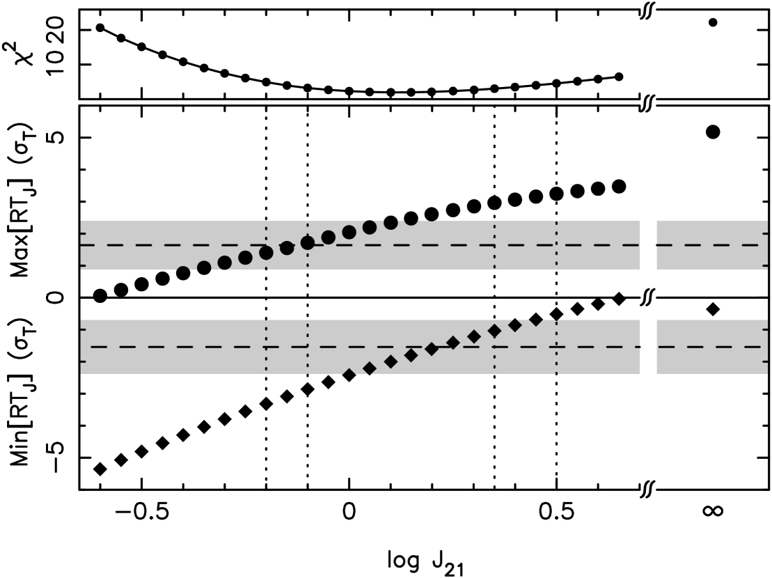
Figure 6: Main panel: most significant positive (dots) and negative (diamonds) deviations (in units of $\sigma_{T}$) of the absorption model from the data in the region most likely affected by the proximity of the QSOs as a function of the mean Lyman limit background intensity $J$. The dashed lines and the grey regions mark the expected and $\pm 1\sigma$ significance levels of these deviations in the case where they are due to random fluctuations (i.e. for the correct model), which were determined from $1000$ simulated datasets. The absence of a proximity effect corresponds to $J=\infty$ and is strongly rejected. Top panel: $\chi^{2}$ of the corresponding points in the main panel. The best fit is achieved for $\log J_{21}=0.1$ with $\chi_{\rm min}^{2}=1.98$. The inner and outer dotted lines in the main panel mark the formal $68$ and $90$ per cent confidence intervals respectively.

4.2.1 Dependence on model parameters

Does the above result depend sensitively on any of the model parameters introduced in Sections 3.2 and 3.3? Because of the transition (13) we must expect the result to depend on $\beta$. At a given $J$, a larger value of $\beta$ increases the model transmission and thus decreases both the maxima and minima of Fig. 6, which will result in a larger measured value for $J$. For $\beta=1.7$ and $1.3$ we find $\log J_{21}=0.6^{+0.3}_{-0.25}$ and $-0.45^{+0.45}_{-0.4}$ respectively. However, increasing $\beta$ also has the effect of decreasing the model variance so that the maxima and minima of Fig. 6 move further apart, which decreases the goodness of fit. For $\beta=1.7$ we find $\chi^{2}=10.1$ and thus the fit is no longer acceptable.

Since the redshift coverage of the present sample is not very large and because we determine the optical depth normalization, $B$, directly from the data, our results cannot depend sensitively on $\gamma$. To confirm this we repeated the above analysis for $\gamma=2.5$ and found $\log J_{21}=0.15^{+0.35}_{-0.3}$.

Cosmological parameters enter the analysis via the last factor in equation (12). $h$ cancels out but the denominator is relatively less sensitive to $q_{0}$ than the numerator. For an open Universe this factor is larger than in the flat case and so a larger $J$ will be measured. For $q_{0}=0.15$ we find $\log J_{21}=0.15^{+0.4}_{-0.3}$ and thus our result does not depend sensitively on the cosmological model.

4.2.2 Emission line shifts

In Section 2 we already noted that the redshifts of the QSOs have probably been underestimated since they were determined from high ionization lines. Assuming that all the emission line redshifts are offset from their true systemic values by a velocity $\Delta v$ to the blue we have repeated the above analysis as a function of $\Delta v$. In Fig. 8 we show our estimate of $J$ for various values of $\Delta v$ (dots, solid line). The reduction of $J$ is very similar to that found by ?) (diamonds, dashed line). From similarly luminous QSOs ?) estimated the mean velocity shift for the ?) QSOs to lie in the range $1300$ km s^-1 $<\Delta v<1600$ km s^-1 and estimated the true background intensity to be $\log J_{21}=-0.3^{+0.2}_{-0.22}$. For our sample of QSOs the $\Delta v$-luminosity relationship given by ?) predicts $\Delta v\approx 800$ km s^-1 which yields $\log J_{21}=-0.45^{+0.4}_{-0.3}$. These results are in good agreement with each other as well as with $\log J_{21}\approx-0.3$ at $z=2.5$–$3$ computed by ?) for a background dominated by the QSO population observed in optical surveys and a $q_{0}=0.1$ cosmology.

Figure 8: Estimated value of the mean Lyman limit background intensity, $J$, assuming that the measured high ionization emission line redshift of every QSO is smaller than the true systemic value by an amount $\Delta v$. Dots, solid line: this work. Diamonds, dashed line (offset by $50$ km s^-1 for clarity): Espey’s (1993) analysis of Lu et al.’s (1991) data for comparison. Error bars are $90$ per cent confidence limits.

4.3 Variation with luminosity and redshift

4.3.1 Significance

Figure 10: (a) Significance of proximity effect in individual QSOs versus QSO Lyman limit luminosity. Solid dots are the data. Open circles are the mean significance levels found in $1000$ simulated datasets, where the simulations include a proximity effect according to the ionization model with $\log J_{21}=-0.45$ (S3). The vertical error bars on the data are the $\pm 1\sigma$ ranges found in these simulations. Open squares: same as open circles but with $J=\infty$ (no proximity effect, S1). (b) Same as (a) but now plotted against QSO redshift. (c) Same as (a) but all significance levels have been scaled to the mean redshift of the sample using equation (22) in order to isolate the effect of luminosity on the proximity effect. The solid, dashed and dotted lines show the best fit $f(L_{\nu},\bar{z}_{\rm Q})$ for the data and the two sets of simulations respectively. (d) Same as (b) but all significance levels have been scaled to the mean luminosity of the sample using equation (22) in order to isolate the effect of redshift on the proximity effect. The solid, dashed and dotted lines show the best fit $f(\bar{L}_{\nu},z_{\rm Q})$ for the data and the two sets of simulations respectively.

In Section 4.1 we noted that the significance of the proximity effect varied somewhat when excluding individual spectra from the combined RTT. We now examine the proximity effect in individual spectra in order to test whether it is correlated with QSO Lyman limit luminosity or redshift. The former correlation would be expected if the proximity effect were due to the increased ionizing flux in the vicinity of QSOs and the latter if in addition $J$ varied with redshift and/or the luminosities and redshifts of the QSOs were correlated.

We thus constructed the RTTs of the individual spectra (using $J=\infty$) and searched for the most significant positive deviations of the model from the data in the same way as described in Section 4.2. In other words, for each QSO we determined the significance of the proximity effect. In Fig. 10(a) we plot these maxima as solid dots against QSO Lyman limit luminosity (calculated from equation (11) and listed in Table 2). For comparison, we analysed two simulated datasets, S1 and S3, in exactly the same way. S1 was already introduced in Section 4.2 (no proximity effect model). S3 incorporates the proximity effect according to the ionization model of Section 3.3 with $\log J_{21}=-0.45$ and assumes that all QSO redshifts have been underestimated by $\Delta v=800$ km s^-1. Writing $M\equiv{\rm Max}[RT_{\infty}]$, we plot as open circles the mean of $M$ found in the $1000$ simulated datasets that include the proximity effect (S3). The open squares are the same for the no proximity effect simulations (S1).

Previous authors have presented similar plots (e.g. BDO’s Fig. 1) where they plotted the relative deficiency of absorption lines within some constant radius of the QSOs. One of the advantages of our method is that this radius is no longer constant but is rather allowed to vary in order to maximise the significance of the missing absorption.

Let us first examine correlations in the simulated data. For S1 there is clearly no correlation with luminosity which is as it should be. For S3 there seems to be a trend of increasing significance with increasing luminosity. However, the correlation does not seem to be as tight as one might expect and there seems to be no well-defined relation between the two. Considering that these points are the mean of $1000$ simulations this can hardly be due to random error. The only other parameter that varies from QSO to QSO in the simulations is the redshift. In Fig. 10(b) we plot the significance levels against QSO redshift. Again, for S1 there is no trend. S3 exhibits the same sort of loose correlation as in Fig. 10(a). The luminosities and redshifts of the QSOs are not significantly correlated. Recall also that $J$ does not vary with redshift in our simulations. Why then should there be a trend with redshift at all? The reason is that a given underdensity of absorption is more significantly detected when the ‘background’ absorption line density is higher than when it is lower (cf. LWC, Fig. 6b). Thus a given QSO will have a more noticeable proximity effect at high redshift (where the line density is higher) than at low redshift, all else being equal.

We thus surmise that the lack of a well-defined relation between the significance of the proximity effect, $M$, and luminosity for S3 in Fig. 10(a) is due to the variation in redshift of the QSOs and that $M$ is a function of both luminosity and redshift even though the QSO luminosities and redshifts are not significantly correlated and $J$ does not vary with redshift.

Figure 12: Significance of proximity effect in individual QSOs versus a linear combination of QSO Lyman limit luminosity and redshift. Symbols have the same meaning as in Fig. 10. The solid and dashed lines show the best fit $f(L_{\nu},z_{\rm Q})$ for the data and S3 respectively. S1 is not shown because for these points the best fit slopes are $m_{L}\approx m_{z}\approx 0$.

To demonstrate this behaviour we first fit $M$ with the function

$$f(L_{\nu},z_{\rm Q})=c+m_{L}L_{\nu}+m_{z}z_{\rm Q}$$ (22)

and then scale the significance levels to the mean redshift, $\bar{z}$, and mean luminosity, $\bar{L}_{\nu}$. The results are plotted in Figs 10(c) and (d) respectively. In Fig. 12 we plot $M$ against $m_{L}L_{\nu}+m_{z}z_{\rm Q}$. We can now see that S3 exhibits almost perfect correlation with both luminosity and redshift and that the linear model (22) gives a reasonably good description of the simulations.

The discussion above implies that in order to properly disentangle possible correlations of the proximity effect with luminosity and redshift they should be determined jointly, not separately. We now investigate this effect in more detail.

First, we need to choose a correlation statistic. Previous authors have often used Spearman’s rank correlation coefficient. However, in our case it is reasonable to assume that $M$ is approximately Gaussian distributed and this is indeed observed in the simulations. Therefore it is not necessary to restrict ourselves to a non-parametric test. In addition we have already shown that the linear model (22) gives a good description of the simulations and from Fig. 12 we can judge that it is also an acceptable model for the real data (see also Fig. 16c). It is therefore reasonable to use the slopes of a linear $\chi^{2}$ fit as correlation measures. This also has the advantage that the arguments of the following paragraphs can be understood analytically. In any case, we found that these arguments are qualitatively reproduced when using Spearman’s rank correlation coefficient.

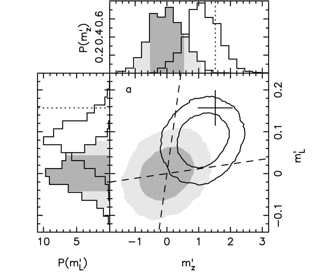
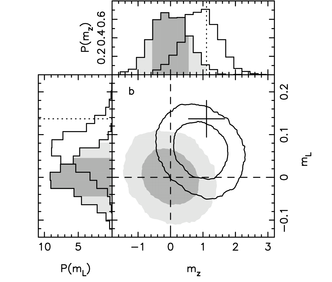
Figure 14: (a) The dark and light grey shaded regions show the 68 and 95 per cent confidence regions of $(m_{z}^{\prime},m_{L}^{\prime})$ derived by independently fitting the significance of the proximity effect in the $1000$ simulated datasets of S1 (no proximity effect) with (23). The contour lines are the same for S3 (ionization model). The cross marks the measured values and formal $1\sigma$ errorbars of $(m_{z}^{\prime},m_{L}^{\prime})$ for the real data. The dashed lines correspond to the lines $m_{z}=0$ and $m_{L}=0$ in panel (b). The upper and left panels show the one-dimensional probability distributions of $m_{z}^{\prime}$ and $m_{L}^{\prime}$ respectively. The dark and light shaded regions in these panels are the one-dimensional 68 and 95 per cent confidence regions respectively. (b) Same as (a) for $(m_{z},m_{L})$, derived by fitting the significance of the proximity effect with (22).

The simplest thing we can now do is to determine the slopes for the $M$-$L_{\nu}$ and $M$-$z_{\rm Q}$ relations independently by fitting the functions

$$\begin{array}[]{lcl}f_{L}(L_{\nu})&=&c_{L}+m_{L}^{\prime}L_{\nu}\\ f_{z}(z_{\rm Q})&=&c_{z}+m_{z}^{\prime}z_{\rm Q}\end{array}$$ (23)

to $M$. We have done this for the $1000$ simulated datasets of both S1 and S3 as well as for the real data. The results are shown in Fig. 14(a). The shaded regions in the main panel are the $68$ and $95$ per cent confidence regions for S1, the contours are the same for S3 and the cross marks the result for the real data.

The first thing we notice is that the values of $(m_{z}^{\prime},m_{L}^{\prime})$ measured in the real data are consistent with the ionization model, but they are inconsistent with the no proximity effect model at $>3\sigma$. However, note that in the simulations $m_{L}^{\prime}$ and $m_{z}^{\prime}$ are not independent. Calculating Pearson’s correlation coefficient we find

$$\rho(m_{L}^{\prime},m_{z}^{\prime})=\hat{\rho}(L_{\nu},z_{\rm Q})=0.14,$$ (24)

where $\hat{\rho}(L_{\nu},z_{\rm Q})$ is the correlation coefficient between $L_{\nu}$ and $z_{\rm Q}$ for the $10$ QSOs used here, not that of the parent population ($=\rho(L_{\nu},z_{\rm Q})$) from which they were drawn, which may well be zero. Thus any measurement in the top right-hand part of the plot deviates from the no proximity effect hypothesis less significantly than what would have been inferred if the correlation between $L_{\nu}$ and $z_{\rm Q}$ had been neglected. Note that it is the actual numerical value of $\hat{\rho}$ that matters here and not whether or not it is consistent with $\rho(L_{\nu},z_{\rm Q})=0$.

What would we expect if the proximity effect were caused by some property, $x$, of the QSO or its environment unrelated to the QSO’s UV flux (‘$x$-model’)? As for the ionization model we would expect a correlation of $M$ with $z_{\rm Q}$ because this is simply the effect of increasing absorption line density with increasing redshift. Since $\hat{\rho}(L_{\nu},z_{\rm Q})\neq 0$ we therefore expect the centre of the shaded ellipses in Fig. 14(a) to move along the line

$$m_{L}^{\prime}=m^{z}_{L}\;m_{z}^{\prime}=\hat{\rho}(L_{\nu},z_{\rm Q})\;\sqrt{\frac{V(z_{\rm Q})}{V(L_{\nu})}}\;m_{z}^{\prime}$$ (25)

(marked by a dashed lined), where $V$ denotes the sample variance. Thus a measurement in the top right-hand part of the plot deviates less significantly from the $x$-model than what would have been inferred if the correlation between $L_{\nu}$ and $z_{\rm Q}$ had been neglected.

This complication can be avoided if we use $(m_{z},m_{L})$ of equation (22) instead of $(m_{z}^{\prime},m_{L}^{\prime})$. Fig. 14(b) shows the result of fitting (22) to the simulations and the data. The relationship between Figs 14(a) and (b) can be most easily understood by writing down the linear co-ordinate transformation which relates $(m_{z}^{\prime},m_{L}^{\prime})$ and $(m_{z},m_{L})$ as

$${m_{z}\choose m_{L}}=\frac{1}{1-\hat{\rho}^{2}}\left(\begin{array}[]{cc}1&-m^{L}_{z}\\ -m^{z}_{L}&1\\ \end{array}\right){m_{z}^{\prime}\choose m_{L}^{\prime}}.$$ (26)

We can now see that they are related by a Lorentz transformation followed by a stretch of $(1-\hat{\rho}^{2})^{-\frac{1}{2}}$ and that the line $m_{L}^{\prime}=m^{z}_{L}\;m_{z}^{\prime}$ is transformed to the line $m_{L}=0$. Thus in this frame of reference we do not have to worry about $\hat{\rho}$ when asking whether the data is compatible with the $x$-model, except for the fact that we now have $\rho(m_{L},m_{z})=-\hat{\rho}(L_{\nu},z_{\rm Q})$.

In Figs 16(a), (b) and (c) we plot the distribution of minimum $\chi^{2}$ values obtained from fitting (23) and (22) respectively. The shaded histogram (S1) follows the $\chi^{2}$-distribution quite well in all cases. However, both the real data (dotted line) and the ionization model (S3, solid histogram) are not well modelled by the independent fits (23).

Thus we conclude that the observed significance of the proximity effect is a linear function of both redshift and luminosity and is well described by a function of the form (22). This observed correlation with luminosity and redshift is inconsistent with the no proximity effect model at the $3.5\sigma$ level. A model that exhibits correlation with redshift but not luminosity is excluded at the $2.6\sigma$ level. These values take into account the correlation between $L_{\nu}$ and $z_{\rm Q}$ of the present dataset. If we had ignored this correlation we would have inferred $4.1\sigma$ and $3.2\sigma$ respectively.

The discussion above enables us to go one step further. Consider again the $x$-model. If $x$ is indeed uncorrelated with $L_{\nu}$ for the general QSO population, i.e. $\rho(x,L_{\nu})=0$, then for our sample we would most likely find $\hat{\rho}(x,L_{\nu})=0$, which we have implicitly assumed in the previous discussion. However, $\hat{\rho}(x,L_{\nu})$ may well be $\neq 0$, either because of random fluctuations or because $\rho(x,L_{\nu})\neq 0$. This would induce a spurious correlation between $M$ and $L_{\nu}$. What value of $\hat{\rho}(x,L_{\nu})$ is required so that the $x$-model is consistent with the data? Assuming $\hat{\rho}(x,z_{\rm Q})=0$ we find that $\hat{\rho}(x,L_{\nu})$ has to lie in the range

$$0.37<\hat{\rho}(x,L_{\nu})<0.80$$ (27)

in order to be consistent with the data at the $1\sigma$ level. Thus in the present dataset, the hypothetical property $x$ would have to be noticeably correlated with luminosity.

Since we do not know the distribution from which $x$ is drawn it is not possible to reliably estimate whether this result excludes the hypothesis that $x$ and $L_{\nu}$ are not correlated in the parent population. However, assuming Gaussianity in both $x$ and $L_{\nu}$, we find that the most likely value of $\hat{\rho}(x,L_{\nu})=0.59$ excludes the hypothesis $\rho(x,L_{\nu})=0$ at the $\sim 96$ per cent confidence level (using Student’s $t$-distribution).

By comparing the data with S3 in Fig. 14(b) it is apparent that the observed dependence of the proximity effect on redshift is entirely accounted for by the evolution of the number density of absorption lines and there is no evidence to suggest that $J$ varies over the redshift range considered here. It is also apparent that this conclusion is not overly sensitive to our choice of $\gamma$, the evolutionary index of the absorption line density. On the other hand, the data do not exclude some (positive or negative) evolution either. In any case, if $J$ is due to the known QSO population then it is expected to peak smoothly in the redshift range covered here [Haardt & Madau (1996)] and thus one would not expect strong evolution.

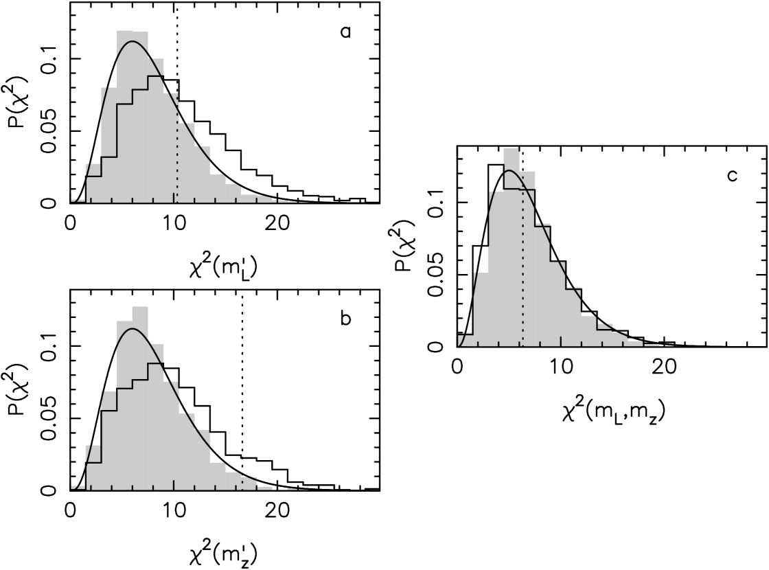
Figure 16: (a) The grey shaded histogram is the distribution of minimum $\chi^{2}$ values obtained from fitting $f_{L}(L_{\nu})$ (equation 23) to the $1000$ simulated datasets of S1 (no proximity effect). The solid histogram is the same for S3 (ionization model). The dashed line marks the value of $\chi^{2}$ for the real data. The smooth solid line shows the $\chi^{2}$-distribution for eight degrees of freedom. (b) Same as (a) for $f_{z}(z_{\rm Q})$. (c) Same as (a) and (b) for $f(L_{\nu},z_{\rm Q})$ (equation 22). The solid line shows the $\chi^{2}$-distribution for seven degrees of freedom.

4.3.2 Size

If the ionization model is correct one would in principle also expect the size of the region affected by the QSO’s UV flux to be correlated with luminosity. We can test for this effect by noting the size of the smoothing function at which the maxima $M$ of Fig. 10 were detected. However, in the simulations we find that the distribution of sizes is very broad and almost one-tailed and thus difficult to characterise. In addition the distributions for S1 and S3 overlap almost completely with only the peak moving to slightly larger values for S3. There is also some evidence that for the ionization model the distribution of sizes moves to larger values for larger luminosities but again the effect is small compared to the extent of the distribution. Thus we are forced to conclude that this is not a powerful test and simply note that the detected sizes in the real data range from $\sim 500$ to $\sim 7000$ km s^-1 and lie well within the $90$ per cent confidence ranges of both S1 and S3 in all cases.

5 Results on foreground proximity effect

5.1 Existence of the effect

We now exploit the fact that the QSOs of Table 2 are a close group in the plane of the sky. Essentially, we repeat here the analysis of Section 4.1: for each pair of background QSO (BQSO) and foreground ionizing source (IS), we shift the spectrum of the BQSO into the restframe of the IS and construct its transmission triangle using $J=\infty$. We now use a Gaussian smoothing function because we are no longer working at the ‘edge’ of the data. We then average all the transmission triangles where they overlap, creating a composite RTT. Thus in equation (20) $T_{i}$ still refers to the measured transmission of the BQSO (but is replaced by $G_{i}$ because we now use a Gaussian smoothing function) and we replace $z_{{\rm Q}i}$ with $z_{{\rm IS}i}$, where $i$ now labels a BQSO-IS pair. If the foreground proximity effect exists, it should be more significant in this composite RTT than in any individual RTTs and is expected to appear as a region of $RG_{\infty}>0$ near $\lambda_{r}=\lambda_{\alpha}$. From now on we exclude all spectral regions within $5000$ km s^-1 of the BQSOs from the analysis in order not to contaminate our results with the background proximity effect.

Before we proceed we need to consider the following complication. For each BQSO-IS pair we can calculate $\omega_{\rm p}=\omega(z=z_{\rm IS},z_{\rm IS},\alpha)$ (assuming $\log J_{21}=-0.45$, cf. equation 12). $\omega_{\rm p}$ is the maximum value a given IS can achieve along the line of sight to a BQSO, separated on the sky by an angle $\alpha$. Pairs with large $\omega_{\rm p}$ should show a strong proximity effect. However, below some value of $\omega_{\rm p}$ the proximity effect will be essentially non-existent. Adding pairs with $\omega_{\rm p}$ below this value to the composite may in fact decrease the overall significance of the effect.

We thus construct several composite RTTs, each with a different lower limit on $\omega_{\rm p}$, which we denote by $\omega_{\rm c}$. Thus $RG_{J}(\omega_{\rm c})$ refers to a composite reduced transmission triangle in which all BQSO-IS pairs with $\omega_{\rm p}>\omega_{\rm c}$ are included.

Each of these RTTs was searched for the most significant positive deviation of the model from the data in the interval [$-1000$ km s^-1$,+2000$ km s^-1] around $\lambda_{\alpha}$. The interval is asymmetric to allow for underestimated QSO redshifts. In Fig. 18 we plot these maxima versus $\omega_{c}$. For comparison we have performed the same analysis on the $1000$ simulated datasets of S1 (no proximity effect). We plot the mean and $\pm 1\sigma$ significance levels as the dashed line and hashed region respectively. Clearly, our data are consistent with the absence of any foreground proximity effect.

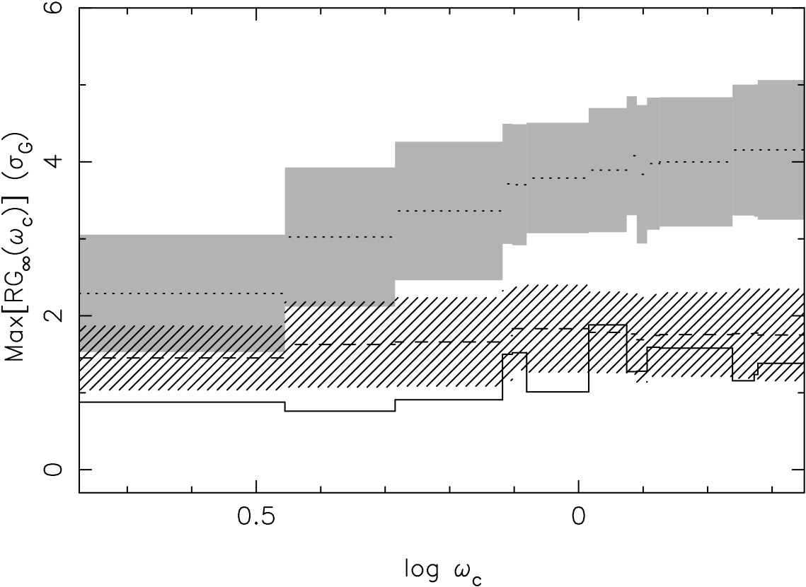
Figure 18: Significance of the foreground proximity effect as derived from composite RTTs which include all BQSO-IS pairs with $\omega_{\rm p}>\omega_{\rm c}$. The solid line is the data. The dotted line and grey shaded regions are the mean and $\pm 1\sigma$ significance levels found in $1000$ simulated datasets that include the foreground proximity effect according to the ionization model with $\log J_{21}=-0.45$ (S4). The dashed line and hashed region are the same for $J=\infty$ (no proximity effect, S1). The number of BQSO-IS pairs included in the RTT increases from $1$ at the left end of the plot to $14$ at the right end.

Given the luminosities and inter-sightline spacings of the present set of QSOs, do we expect to be able to detect a signal? To answer this question we have created a fourth set of $1000$ simulations (S4). These include the effects of all foreground IS with $\omega_{\rm p}>0.5$ and $\log J_{21}=-0.45$. Subjecting S4 to the same analysis as above yields the dotted line and grey shaded region in Fig. 18. Evidently, if $J$ has indeed the value that was measured from the background proximity effect and if QSOs radiate isotropically, then we should be able to detect the foreground proximity effect at the $2-4\sigma$ level in our data.

5.2 Lower limit on $J$

The above result implies that we can at least derive a lower limit to $J$ under the assumption that QSOs radiate isotropically. Setting $\omega_{\rm c}=0.5$ we have repeated the analysis of Section 4.2 using a foreground RTT that includes $14$ BQSO-IS pairs. The result is shown in Fig. 20. We can see that the data are consistent with a large range of values of $J$, including $J=\infty$. However, for small values of $J$ the model predicts too little absorption to be compatible with the data. From this constraint we derive a lower limit of $\log J_{21}>0.3$ ($90$ per cent confidence).

From Fig. 8 we can see that this lower limit is larger than the upper limit derived from the background proximity effect for all $\Delta v\mathrel{\mathchoice{\vbox{\offinterlineskip\halign{\hfil$\reset@font\displaystyle#$\hfil\cr>\cr\sim\cr}}}{\vbox{\offinterlineskip\halign{\hfil$\reset@font\textstyle#$\hfil\cr>\cr\sim\cr}}}{\vbox{\offinterlineskip\halign{\hfil$\reset@font\scriptstyle#$\hfil\cr>\cr\sim\cr}}}{\vbox{\offinterlineskip\halign{\hfil$\reset@font\scriptscriptstyle#$\hfil\cr>\cr\sim\cr}}}}200$ km s^-1. If we did not underestimate $J$ in Section 4.2 then the simplest explanation for this discrepancy is that QSOs radiate anisotropically. If we require that the lower limit derived from the lack of a foreground proximity effect coincides with the upper limit of the background measurement then the QSOs of our sample must emit less ionizing radiation in the plane of the sky than along the line of sight to Earth by at least a factor of $1.4$ for $\Delta v>400$ km s^-1. This number increases to $2.2$ for $\Delta v>800$ km s^-1.

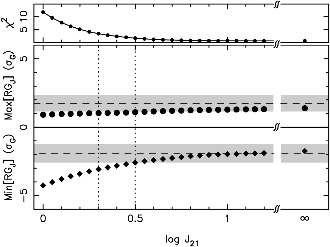
Figure 20: This plot is the equivalent of Fig. 6 for the foreground proximity effect. In the main panel we show the most significant positive (dots) and negative (diamonds) deviations (in units of $\sigma_{G}$) of the absorption model from the data in the regions near the positions of close-by foreground QSOs as a function of the mean Lyman limit background intensity $J$. The dashed lines and the grey regions mark the expected and $\pm 1\sigma$ significance levels of these deviations in the case where they are due to random fluctuations. The data are consistent with the absence of a foreground proximity effect ($J=\infty$). Thus we cannot derive an upper limit on $J$. The two dotted lines mark the $68$ and $90$ per cent confidenc lower limits on $J$.

5.3 The Q0042–2639 quadrangle

Having established that the dataset as a whole does not exhibit any evidence for the existence of the foreground proximity effect, we now present a possible exception to this rule. From Fig. 4 we can see that Q0042–2639 is surrounded by four nearby background QSOs. Interestingly, all four show underdense absorption near the position of the foreground QSO. In Table 4 we list the BQSO name, the angular separation from the foreground QSO, the significance of the underdensity, $M$ (in units of $\sigma_{G}$), the velocity offset of the underdensity from the foreground QSO redshift and finally the size of the underdensity (FWHM of the smoothing Gaussian). In the last line we list the same quantities for the composite RTT of the four BQSOs. Note that the offsets from the foreground QSO’s redshift are of the same magnitude but of opposite sign for the two pairs of opposing BQSOs (cf. Fig. 4). However, this is no longer true if we add $\mathrel{\mathchoice{\vbox{\offinterlineskip\halign{\hfil$\reset@font\displaystyle#$\hfil\cr>\cr\sim\cr}}}{\vbox{\offinterlineskip\halign{\hfil$\reset@font\textstyle#$\hfil\cr>\cr\sim\cr}}}{\vbox{\offinterlineskip\halign{\hfil$\reset@font\scriptstyle#$\hfil\cr>\cr\sim\cr}}}{\vbox{\offinterlineskip\halign{\hfil$\reset@font\scriptscriptstyle#$\hfil\cr>\cr\sim\cr}}}}400$ km s^-1 to the foreground QSO’s redshift.

At first glance, it may seem exceedingly unlikely to find an underdensity in four different lines of sight at a similar position (which happens to coincide with a foreground QSO) by chance. However, the spread of the underdensities in redshift is actually fairly large. Thus when we combine the four lines of sight to a composite RTT the significance level of the ‘void’ rises only marginally from $\sim 3\sigma_{G}$ in individual lines of sight to $3.5\sigma_{G}$ in the composite. Nevertheless, in the $1000$ simulated datasets of S1 we find that the largest random fluctuations in the composite RTT have a mean significance level of $(1.69\pm 0.53)\sigma_{G}$ and thus it seems that the void is in fact genuine. Indeed, a measurement of $J$ from the composite RTT yields $\log J_{21}=-0.65^{+0.6}_{-0.5}$ which is lower than, but consistent with our measurements from the background proximity effect. From Fig. 10 (and Table 2) we can see that Q0042–2639 also shows a slightly (but not significantly) more prominent background proximity effect than ‘predicted’ by the other QSOs for its luminosity and redshift. Together these observations may be an indication that the luminosity of Q0042–2639 has been underestimated.

Table 4: The Q0042–2639 quadrangle.

BQSO	$\alpha$	$M$	$\Delta$	FWHMs
	arcmin	$\sigma_{G}$	km s-1	km s-1
Q0043–2633	$13.6$	$2.97$	$-460$	$1260$
Q0042–2627	$11.7$	$3.11$	$-2390$	$5530$
Q0041–2638	$11.9$	$2.71$	$+230$	$3120$
Q0042–2656	$17.6$	$3.03$	$+2630$	$1210$
Composite		$3.52$	$+160$	$1880$

6 Uncertainties

In Section 4.2 we have already quantified the effect of uncertainties in model parameters, QSO redshifts and cosmology. We now discuss a number of other uncertainties associated with the present study.

It is clear that our method is sensitive to errors in the continuum placement, probably more so than the generic ‘line counting’ method. In ?) we attempted to account for random errors in the lowest orders of the continuum fit by determining the normalization of the mean optical depth, $B$, for each spectrum separately. Here we used a single value of $B$ derived from the entire dataset. This has the advantage of making our estimate of $J$ fairly insensitive to the adopted value of $\gamma$ (the evolutionary power law index). The disadvantage is that errors in the continuum placement should, in principle, increase the scatter when comparing the significance of the proximity effect in individual lines of sight (cf. Fig. 10). However, this comparison is based on measurements near the Ly$\alpha$ emission lines of the QSOs where the S/N is in general quite high and thus the continuum more secure. A systematic over- or underestimation of continua can only affect our results if such a bias is different for different parts of the spectra. This difference could be caused by the higher S/N and greater curvature of the continuum in the wing of the Ly$\alpha$ emission line.

As our method deals only with the transmitted flux it circumvents all problems that arise from defining a sample of individual absorption lines. These problems include line blending, curve of growth effects (e.g. [Scott et al. (2000)]) and Malmquist bias [Cooke et al. (1997)].

The environment of QSOs may well differ from the intergalactic environment in other aspects than just the intensity of ionizing radiation. Most importantly, there may be additional absorption in the vicinity of QSOs above and beyond the absorption already accounted for in our model. If QSOs are hosted by groups or clusters of galaxies then the gravitational pull of the host will cause infall of the surrounding material and may thus increase the absorption line density near a QSO [Loeb & Eisenstein (1995)]. If this effect is not taken into account, the proximity effect will appear weaker than it should and a larger value of $J$ will be inferred. ?) suggested that the magnitude of this effect may be as large as a factor of $\sim 3$. If QSO luminosity is correlated with host mass, then more luminous QSOs are affected more strongly by clustering and the value of $J$ derived from the brightest QSOs should be higher than that derived from the faintest. On the other hand, if all QSOs were affected by clustering in the same way, then one might expect the observed slope of the significance-luminosity relation in Fig. 10 to be larger than the one expected on the basis of the measured (and overestimated) $J$. This is actually the case, although not significantly so. However, all of the QSOs in the present sample are radio-quiet. The hypothesis that such QSOs reside in rich galaxy cluster environments has been repeatedly rejected at low redshifts and there seems to be little evolution in the environment of radio-quiet QSOs up to $z<1.5$ ([Croom & Shanks (1999)]; [Smith et al. (2000)]). In any case, it is most likely very difficult to disentangle clustering from the proximity effect and we believe that this issue deserves further study. For now, it remains an uncertainty.

In Section 3.3 we assumed that the column density of an absorber is proportional to the inverse of the incident ionizing flux. This is only true for absorbers composed purely of hydrogen. However, ?) found that the inclusion of metals into the model has an insignificant effect on the derived value of $J$.

We have also ignored the fact that as radiation travels from a QSO to a given absorber it will be attenuated by all the intervening absorbers. In particular, an intervening strong Lyman limit system will essentially ‘black out’ the QSO entirely. In principle, disregarding this effect causes overestimation of $J$ but ?) concluded that the effect is negligible for $\log N<17$. Higher column densities produce a conspicuous continuum break at the Lyman limit. Unfortunately, only three of our spectra cover any part of the Lyman limit region. One of these, Q0042–2656, shows a Lyman break but the system lies $\sim 5200$ km s^-1 away from the QSO. In any case, since high column density absorbers are comparatively rare we would expect that only a fraction of our QSOs are afflicted by this problem. However, from Fig. 10 it is apparent that none of our QSOs shows a proximity effect which is unusually small for its luminosity and redshift. We thus find it unlikely that we have significantly overestimated $J$ due to this effect.

Obscuration by dust in intervening damped Ly$\alpha$ absorption systems may cause a QSO’s luminosity and consequently $J$ to be underestimated [Srianand & Khare (1996)]. Since there are no known damped Ly$\alpha$ absorption systems or candidates in our sample we believe that our value of $J$ is not affected by dust obscuration.

However, there are a number of other factors that create uncertainty in the estimated luminosities of the QSOs. Errors in $K$-corrections and the QSO continuum slope could be avoided by direct spectrophotometric observations, but there are at least two other more fundamental and probably larger uncertainties:

1. QSO variability. The equilibration time-scale of Ly$\alpha$ absorbers, $t_{\rm eq}$, is of the order $10^{4}$ years. Thus the observed ionization state of an absorber in the vicinity of a QSO will approximately reflect the ionizing flux received from that QSO averaged over the $10^{4}$ years prior to the epoch of observation, $\bar{L}$. Let us assume that the intrinsic luminosity of QSOs varies on a single time-scale, $t_{\rm V}$. For $t_{\rm V}\mathrel{\mathchoice{\vbox{\offinterlineskip\halign{\hfil$\reset@font\displaystyle#$\hfil\cr<\cr\sim\cr}}}{\vbox{\offinterlineskip\halign{\hfil$\reset@font\textstyle#$\hfil\cr<\cr\sim\cr}}}{\vbox{\offinterlineskip\halign{\hfil$\reset@font\scriptstyle#$\hfil\cr<\cr\sim\cr}}}{\vbox{\offinterlineskip\halign{\hfil$\reset@font\scriptscriptstyle#$\hfil\cr<\cr\sim\cr}}}}t_{\rm eq}$ the QSO’s observed luminosity may be different from $\bar{L}$ and thus the strength of the observed proximity effect may be different from that expected on the basis of the ionization model. The same may be true for the foreground proximity effect even when $t_{\rm V}>t_{\rm eq}$ if $t_{\rm V}$ is smaller than the light travel time from the IS to the observed absorption ($\approx 10^{6}$ years). Obviously, we have no information on QSO variability on such large time-scales. However, ?) found that on time-scales of $100$ to $1000$ days the distribution of brightness deviations about the mean light curves of $42$ QSOs has a width of $0.14$ mag in the $B$-band. Thus, variability on short time-scales contributes substantially to the uncertainty in the QSOs’ luminosities.

2. Gravitational lensing. None of the QSOs in our sample are known to be lensed and at least four of them have been included in searches for multiply imaged QSOs with negative results [Surdej et al. (1993)], implying that they are at least not strongly lensed. However, some or all of them may be weakly lensed by the non-homogeneous distribution of foreground matter on large scales. There are two known overdensities of C iv absorption systems in the foreground of the present QSO sample [Williger et al. (1996)] which could possibly cause weak lensing ([Vanden Berk et al. (1996)]; [Holz & Wald (1998)]). Ray-tracing experiments performed on simulations of cosmological structure formation have yielded the probability distribution function of the magnification caused by galaxy clusters and large-scale structure [Hamana et al. (2000), Wambsganss et al. (1998)]. At $z=3$ the dispersion of this distribution can be as high as $0.4$ (with a mean of $1$) and the distribution has a power law tail towards large magnification. For the standard model the probability of encountering a magnification of $2$ or greater is a few per cent but for a $\Lambda$ model it is less than $10^{-3}$. A magnification by a factor of $1.2$ (or a demagnification by a factor $1.2^{-1}$) introduces an additional uncertainty of $\pm 2.5\log 1.2=\pm 0.2$ mag which is actually larger than the quoted measurement errors on the observed $B$-band magnitudes.

What are the effects of luminosity uncertainties on our results if we treat them as random errors? Any statistical errors should increase the error on $J$. We can estimate the magnitude of this effect by the following argument. If we measured $J$ from a single QSO then the additional error on $J$ should be on the order of $\Delta(\log J)\approx 0.4\Delta m$, where $\Delta m$ is the error on the QSO’s magnitude. For ten QSOs this error should be smaller by a factor of $\sqrt{10}$. Thus for $\Delta m=0.5$ mag we find $\Delta(\log J)=0.063$ which is much smaller than the quoted error of $0.4$.

This also shows that the known QSO variability, gravitational lensing and measurement errors on the QSO magnitudes cannot increase the errorbars on our foreground and background estimates of $J$ by an amount large enough to make these two values compatible.

However, statistical errors in $L_{\nu}$ will weaken our results on the correlation between the significance of the proximity effect and $L_{\nu}$. Clearly, for errors as large as $\Delta m=0.5$ mag (which corresponds to a factor of $1.6$ in luminosity) fitting a straight line to the data points in Fig. 10 will be almost meaningless. In Section 4.3 we estimated that the significance of the proximity effect is correlated with luminosity at the $2.6\sigma$ level. For $\Delta m=0.3$ mag this significance drops to $2.1\sigma$. Thus measurement errors and the known variability of QSOs alone cannot entirely invalidate the evidence for a correlation of the background proximity effect with QSO Lyman limit luminosity.

In any case it is probably more appropriate to treat both QSO variability and gravitational lensing as systematic errors. Because of the steepness of the bright end of the QSO luminosity function a magnitude limited sample of QSOs is more likely to contain magnified QSOs than demagnified ones (e.g. [Pei (1995)]; [Hamana et al. (2000)]). The same is true for QSOs that are near a peak in their lightcurves (e.g. [Francis (1996)]). Thus either of these effects could cause a systematic overestimation of $J$. Together they imply that on average the QSO magnitudes may have been overestimated by $\sim 0.35$ mag which corresponds to an overestimation of $J$ by $\Delta(\log J)=0.14$.

Note that gravitational lensing and QSO variability on short time-scales ($<10^{4}$ years) affect our $J$ estimates from the classical and foreground proximity effects in the same way. However, if QSO luminosities vary on time-scales of $\sim 10^{6}$ years then this will affect only the latter estimate as explained above. In this case we would expect the QSOs to have been systematically fainter over a period of $\sim 10^{6}$ years prior to the time they emitted the photons which we receive today, causing us to overestimate $J$ when measuring it from the foreground proximity effect. To reconcile the foreground and background values of $J$ we require a variability of $\Delta m=2.5\log 2.2=0.86$ mag (assuming $\Delta v=800$ km s^-1) on time-scales of $\sim 10^{6}$ years.

Past authors [Cooke et al. (1997), Scott et al. (2000)] have attempted to test for the presence of gravitational lensing in their data: since high luminosity QSOs are more likely to be lensed than low luminosity ones, an estimate of $J$ from the former group should be higher than from the latter. From Fig. 10 we can see that the higher luminosity QSOs of our sample actually show a slightly more prominent proximity effect than expected for $\log J_{21}=-0.45$. Thus a $J$ measurement from these four QSOs will yield a lower value, contrary to the expectation if they were lensed.

7 Conclusions

We have analysed the Ly$\alpha$ forest spectra of a close group of $10$ QSOs in search of the (foreground) proximity effect using a novel method based on the statistics of the transmitted flux. We list our various measurements of $J$ in Table 6 and we summarise our main results as follows:

1. We confirm the existence of the classical background proximity effect at the $>99$ per cent confidence level.

2. From the observed underdensity of absorption near the background QSOs we derive $\log J_{21}=0.1^{+0.4}_{-0.3}$ (90 per cent confidence limits).

3. Correcting all QSO redshifts by $\Delta v=+800$ km s^-1 we find $\log J_{21}=-0.45^{+0.4}_{-0.3}$. The reduction of $J$ with $\Delta v$ is consistent with previous results.

4. The significance of the background proximity effect in individual lines of sight is correlated with QSO Lyman limit luminosity at the $2.6\sigma$ level, thus lending further support to the hypothesis that the proximity effect is caused by the additional UV flux from background QSOs. We account for the fact that the significance is also correlated with redshift which is due to the evolution of the absorption line density. We considered an alternative model for the proximity effect where the underdense absorption is caused by some hypothetical property $x$ of the QSO or its environment. We find that the property $x$ would have to be noticeably correlated with luminosity in our sample and probably in the QSO population in general.

5. The full sample shows no evidence for the existence of the foreground proximity effect.

6. This absence implies a lower limit of $\log J_{21}>0.3$. If we interpret the discrepancy of this lower limit with previous measurements as evidence that QSOs radiate anisotropically, then they must emit at least a factor of $1.4$ less ionizing radiation in the plane of the sky than along the line of sight to Earth.

7. Our sample includes the fortunate constellation of a foreground QSO surrounded on all sides by four background QSOs with approximately equal separations from the foreground QSO. Contrary to the rest of the sample, this particular QSO induces a foreground proximity effect in the surrounding lines of sight at the $3.5\sigma$ level. For this subsample we measure $\log J_{21}=-0.65^{+0.6}_{-0.5}$.

8. Finally, we have discussed possible sources of systematic and additional statistical errors. We conclude that clustering of absorption systems around QSOs is the most likely source of systematic error. We also find that the known variability of QSOs reduces the significance of the proximity effect-luminosity correlation to $2.1\sigma$.

Table 6: Summary of $J$ measurements and limits.

	$\log J_{21}$	Errorsa
standard	$0.10$	$+0.40,-0.30$
$\beta=1.3$	$-0.45$	$+0.45,-0.40$
$\beta=1.7$	$0.60$	$+0.30,-0.25$
$\gamma=2.5$	$0.15$	$+0.35,-0.30$
$q_{0}=0.15$	$0.15$	$+0.40,-0.30$
$\Delta v=400$ km s-1	$-0.25$	$+0.40,-0.30$
$\Delta v=800$ km s-1	$-0.45$	$+0.40,-0.30$
foreground	$>0.30$
Q0042–2639 quadrangle	$-0.65$	$+0.60,-0.50$

^aErrors are $90$ per cent confidence limits.

From Fig. 2 we can see that our measurement of $J$ from the background proximity effect is consistent with most previous measurements. ?) found a somewhat larger value $\log J_{21}=0.5$ but she did not correct the QSO redshifts, remarking only that a correction of $\Delta v=1000$ km s^-1 would lower her value of $J$ by a factor of $3$. ?) also found a considerably higher value which is partly due to the fact that they used $\beta=1.7$. [Kulkarni & Fall (1993)]’s (?) low value of $J_{21}=-2.2$ at $z\approx 0.5$ is usually taken as evidence for an evolving background.

?) and ?) noted that the relative deficit of absorption lines near background QSOs was larger for the high-luminosity halves of their samples than for the low-luminosity ones. However, they did not quantify this effect in any detail and did not compare it to the expectations from the ionization model. BDO identified a trend of the line deficit with luminosity at $1\sigma$ significance. ?) on the other hand found no such trend. In Figs. 10, 12 and 14 we have presented good evidence that the significance of the proximity effect is indeed correlated with QSO luminosity and redshift. This result was possible because we used a technique that is more sensitive to variations of the absorption density on large scales than the generic line counting method. Using simulations we find that these correlations are entirely consistent with the expectations of the ionization model. However, considering the discussion of Section 6 we clearly need to apply our method to a larger sample with a wider range in luminosity to establish this result more firmly. Nevertheless, the present analysis provides further evidence that the interpretation of the proximity effect as being due to increased ionization caused by the extra UV flux from the background QSO is essentially correct.

Although their results were poorly constrained, it is interesting to note that the three BQSO-IS pairs of ?) favoured a similarly high value of $J$ as our full sample of $14$ pairs. The non-detections of the foreground proximity effect by ?) and ?) also imply a high value of $J$. On the other hand, all possible positive detections of the foreground proximity effect ([Dobrzycki & Bechtold (1991)]; [Srianand (1997)]; the Q0042–2639 quadrangle) yield $J$ values that are in line with the measurements from the background effect.

One possible explanation is that most of the QSOs were substantially fainter over a period of $\sim 10^{6}$ years prior to the time they emitted the photons which we receive today. This would cause an overestimate of $J$ when measured from the foreground proximity effect but would not affect the results of the background proximity effect.

As we have already pointed out, the other explanation is that QSOs radiate anisotropically. There is a large body of observational evidence which suggests that the observed characteristics of an Active Galactic Nucleus (AGN) depend on the direction from which it is viewed (see e.g. [Antonucci (1993)] for a review). The basic theme of unified models for AGN is that some or even all of the many different types of AGN are in fact the same type of object but seen from different directions. In these models the directionality is caused by a thick, dusty and opaque torus which surrounds the central engine. The smooth continuum and broad emission lines of a QSO are thought to originate from within the torus and thus they can only be seen indirectly by scattered light when the torus is viewed approximately edge on.

This scenario has two obvious implications: i) all QSOs show a background proximity effect and ii) whether a foreground proximity effect is seen or not depends on whether nearby absorption systems probed by other sightlines can ‘see’ inside the torus of the QSO. If so, they will roughly see the same continuum as we do, resulting in a measurable depletion of absorption and a corresponding $J$ value which is similar to that derived from the background effect. If not, there will be little or no foreground effect, resulting in a high value or lower limit for $J$.

Assuming a simple picture of this kind, ?) used the velocity offset of their void from the foreground QSO to derive a value of $\sim 140$^∘ for the opening angle of the torus.

However, it is difficult to explain the case of the Q0042–2639 quadrangle with this scenario. If all of the four underdensities are real and caused by the forground QSO then it has to emit similar amounts of radiation along three nearly perpendicular axes (north-south, east-west and towards Earth), leaving little room for anisotropic emission.

The current situation is thus uncertain and intriguing enough to stimulate further observations. The motivations and potential gain are clear: by investigating the radiative effects of QSOs (or other AGN) on nearby absorption systems along other lines of sight we can ‘view’ them from different directions which may help to constrain unified models of AGN. The ideal targets for further observations are dense groups of QSOs at similar redshifts. These are rare in current QSO catalogues but, fortunately, currently ongoing redshift surveys like 2QZ will soon remedy this situation.

References

- Allen (1991) Allen C. W., 1991, Astrophysical Quantities. The Athlone Press, London
- Antonucci (1993) Antonucci R., 1993, ARA&A, 31, 473
- Bajtlik et al. (1988) Bajtlik S., Duncan R. C., Ostriker J. P., 1988, ApJ, 327, 570
- Bechtold (1994) Bechtold J., 1994, ApJS, 91, 1
- Bechtold et al. (1987) Bechtold J., Weymann R. J., Zuo L., Malkan M. A., 1987, ApJ, 315, 180
- Blair & Gilmore (1982) Blair M., Gilmore G., 1982, PASP, 94, 742
- Cardelli et al. (1989) Cardelli J. A., Clayton G. C., Mathis J. S., 1989, ApJ, 345, 245
- Carswell et al. (1982) Carswell R. F., Whelan J. A. J., Smith M. G., A. B., Tytler D., 1982, MNRAS, 198, 91
- Chernomordik & Ozernoy (1993) Chernomordik V. V., Ozernoy L. M., 1993, ApJ, 404, L5
- Clayton & Cardelli (1988) Clayton G. C., Cardelli J. A., 1988, AJ, 96, 695
- Cooke et al. (1997) Cooke A. J., Espey B., Carswell R. F., 1997, MNRAS, 284, 552
- Cristiani et al. (1995) Cristiani S., D’Odorico S., Fontana A., Giallongo E., Savaglio S., 1995, MNRAS, 273, 1016
- Cristiani & Vio (1990) Cristiani S., Vio R., 1990, A&A, 227, 385
- Croft et al. (1999) Croft R. A. C., Weinberg D. H., Pettini M., Hernquist L., Katz N., 1999, ApJ, 520, 1
- Croom & Shanks (1999) Croom S. M., Shanks T., 1999, MNRAS, 303, 411
- Crotts (1989) Crotts A. P. S., 1989, ApJ, 336, 550
- Davé et al. (1999) Davé R., Hernquist L., Katz N., Weinberg D. H., 1999, ApJ, 511, 521
- Dinshaw et al. (1998) Dinshaw N., Foltz C. B., Impey C. D., Weyman R. J., 1998, ApJ, 494, 567
- Dobrzycki & Bechtold (1991) Dobrzycki A., Bechtold J., 1991, ApJ, 377, L69
- Drinkwater (1987) Drinkwater M., 1987, Ph.D. thesis, University of Cambridge
- Espey (1993) Espey B. R., 1993, ApJ, 411, L59
- Evans & Hart (1977) Evans A., Hart D., 1977, A&A, 58, 241
- Fardal et al. (1998) Fardal M. A., Giroux M. L., Shull J. M., 1998, AJ, 115, 2206
- Fernández-Soto et al. (1995) Fernández-Soto A., Barcons X., Carballo R., Webb J. K., 1995, MNRAS, 277, 235
- Francis (1993) Francis P. J., 1993, ApJ, 407, 519
- Francis (1996) Francis P. J., 1996, Proc. Astron. Soc. Aust., 13, 212
- Gaskell (1982) Gaskell C. M., 1982, ApJ, 263, 79
- Giallongo et al. (1996) Giallongo E., Cristiani S., D’Odorico S., Fontana A., Savaglio S., 1996, ApJ, 466, 46
- Giallongo et al. (1993) Giallongo E., Cristiani S., Fontana A., Trevese D., 1993, ApJ, 416, 137
- Giveon et al. (1999) Giveon U., Maoz D., Kaspi S., Netzer H., Smith P. S., 1999, MNRAS, 306, 637
- Haardt & Madau (1996) Haardt F., Madau P., 1996, ApJ, 461, 20
- Hamana et al. (2000) Hamana T., Martel H., Futamase T., 2000, ApJ, 529, 56
- Hewitt et al. (1995) Hewitt P. C., Foltz C. B., Chaffee F. H., 1995, AJ, 109, 1498
- Holz & Wald (1998) Holz D. E., Wald R. M., 1998, Phys. Rev. D, 063501
- Hu et al. (1995) Hu E. M., Kim T.-S., Cowie L. L., Songaila A., Rauch M., 1995, AJ, 110, 1526
- Hui (1999) Hui L., 1999, ApJ, 516, 519
- Jenkins & Ostriker (1991) Jenkins E. B., Ostriker J. P., 1991, ApJ, 376, 33
- Kim et al. (1997) Kim T.-S., Hu E. M., Cowie L. L., Songaila A., 1997, AJ, 114, 1
- Kirkman & Tytler (1997) Kirkman D., Tytler D., 1997, ApJ, 484, 672
- Kulkarni & Fall (1993) Kulkarni V. P., Fall S. M., 1993, ApJ, 413, L63
- Liske (2000) Liske J., 2000, MNRAS, 319, 557
- Liske et al. (1998) Liske J., Webb J. K., Carswell R. F., 1998, MNRAS, 301, 787
- Liske et al. (2000) Liske J., Webb J. K., Williger G. M., Fernández-Soto A., Carswell R. F., 2000, MNRAS, 311, 657
- Loeb & Eisenstein (1995) Loeb A., Eisenstein D. J., 1995, ApJ, 448, 17
- Lu et al. (1996) Lu L., Sargent W. L. W., Womble D. S., Takada-Hidai M., 1996, ApJ, 472, 509
- Lu et al. (1991) Lu L., Wolfe A. M., Turnshek D. A., 1991, ApJ, 367, 19
- Møller & Kjærgaard (1992) Møller P., Kjærgaard P., 1992, A&A, 258, 234
- Murdoch et al. (1986) Murdoch H. S., Hunstead R. W., Pettini M., Blades J. C., 1986, ApJ, 309, 19
- Nusser & Haehnelt (1999) Nusser A., Haehnelt M., 1999, MNRAS, 313, 364
- O’Donnell (1994) O’Donnell J. E., 1994, ApJ, 422, 158
- Oke & Korycansky (1982) Oke J. B., Korycansky D. G., 1982, ApJ, 255, 11
- Pei (1995) Pei Y. C., 1995, ApJ, 440, 500
- Press & Rybicki (1993) Press W. H., Rybicki G. B., 1993, ApJ, 418, 585
- Press et al. (1993) Press W. H., Rybicki G. B., Schneider D. P., 1993, ApJ, 414, 64
- Rauch et al. (1997) Rauch M. et al., 1997, ApJ, 489, 7
- Savaglio et al. (1997) Savaglio S., Cristiani S., D’Odorico S., Fontana A., Giallongo E., Molaro P., 1997, A&A, 318, 347
- Schlegel et al. (1998) Schlegel D. J., Finkbeiner D. P., Davis M., 1998, ApJ, 500, 525
- Scott et al. (2000) Scott J., Bechtold J., Dobrzycki A., Kulkarni V. P., 2000, ApJS, 130, 67
- Smith et al. (2000) Smith R. J., Boyle B. J., Maddox S. J., 2000, MNRAS, 313, 252
- Srianand (1997) Srianand R., 1997, ApJ, 478, 511
- Srianand & Khare (1996) Srianand R., Khare P., 1996, MNRAS, 280, 767
- Surdej et al. (1993) Surdej J. et al., 1993, AJ, 105, 2064
- Susa & Umemura (2000) Susa H., Umemura M., 2000, ApJ, 537, 578
- Tytler (1987) Tytler D., 1987, ApJ, 321, 69
- Tytler & Fan (1992) Tytler D., Fan X.-M., 1992, ApJS, 79, 1
- Vanden Berk et al. (1996) Vanden Berk D. E., Quashnock J. M., York D. G., 1996, ApJ, 469, 78
- Wambsganss et al. (1998) Wambsganss J., Cen R., Ostriker J. P., 1998, ApJ, 494, 29
- Warren et al. (1991) Warren S. J., Hewitt P. C., Irwin M. J., Osmer P. S., 1991, ApJS, 76, 1
- Warren et al. (1991) Warren S. J., Hewitt P. C., Osmer P. S., 1991, ApJS, 76, 23
- Webb et al. (1992) Webb J. K., Barcons X., Carswell R. F., Parnell H. C., 1992, MNRAS, 255, 319
- Weinberg et al. (1997) Weinberg D. H., Miralda-Escudé J., Hernquist L., Katz N., 1997, ApJ, 490, 564
- Williger et al. (1994) Williger G. M., Baldwin J. A., Carswell R. F., Cooke A. J., Hazard C., Irwin M. J., McMahon R. G., Storrie-Lombardi L. J., 1994, ApJ, 428, 574
- Williger et al. (1996) Williger G. M., Hazard C., Baldwin J. A., McMahon R. G., 1996, ApJS, 104, 145
- Williger et al. (2000) Williger G. M., Smette A., Hazard C., Baldwin J. A., McMahon R. G., 2000, ApJ, 532, 77
- Zuo (1992) Zuo L., 1992, MNRAS, 258, 45
- Zuo & Bond (1994) Zuo L., Bond J. R., 1994, ApJ, 423, 73
- Zuo & Lu (1993) Zuo L., Lu L., 1993, ApJ, 418, 601