Abstract

We describe the subject of Cosmic Microwave Background (CMB) analysis — its past, present and future. The theory of Gaussian primary anisotropies, those arising from linear physics operating in the early Universe, is in reasonably good shape so the focus has shifted to the statistical pipeline which confronts the data with the theory: mapping, filtering, comparing, cleaning, compressing, forecasting, estimating. There have been many algorithmic advances in the analysis pipeline in recent years, but still more are needed for the forecasts of high precision cosmic parameter estimation to be realized. For secondary anisotropies, those arising once nonlinearity develops, the computational state of the art currently needs effort in all the areas: the Sunyaev-Zeldovich effect, inhomogeneous reionization, gravitational lensing, the Rees-Sciama effect, dusty galaxies. We use the Sunyaev-Zeldovich example to illustrate the issues. The direct interface with observations for these non-Gaussian signals is much more complex than for Gaussian primary anisotropies, and even more so for the statistically inhomogeneous Galactic foregrounds. Because all the signals are superimposed, the separation of components inevitably complicates primary CMB analyses as well.

1 Introduction

1.1 What is CMB Analysis? The subject we call “CMB analysis” is a blend of basic theory, simulation and statistical data analysis. The goal of CMB analyzers is to extract the physics of the various signals that contribute to the data. CMB analyzers may therefore be theorists or experimentalists. Depending upon how advanced the state-of-the-art is, the relevant analysis topic may lean more towards the theory/simulation side or more towards the statistical analysis and Monte Carlo simulation side. In the CMB field, we adopt a theorist’s distinction between primary, secondary and foreground anisotropies, though of course the observations do not know of this distinction. The primary ones are those we can calculate using linear perturbation theory (or, in the case of cosmic defects, with linear response theory). This covers the crucially important epoch of photon decoupling near redshift 1100, and even until the current time on very large scales, and to redshifts of a few on intermediate scales. Secondary anisotropies are those associated with nonlinear phenomena, either calculable via weakly nonlinear perturbation theory, semi-analytic methods or by more direct simulation of nonlinear patterns. Gravitational lensing effects on the CMB, quadratic nonlinearities and the kinetic Sunyaev-Zeldovich effect associated with Thomson scattering from flowing matter, reionization inhomogeneities, the thermal Sunyaev-Zeldovich effect associated with Compton upscattering from hot gas, the Rees-Sciama effect associated with nonlinear potential wells, all come under this heading. We also traditionally call emission by dust in high redshift galaxies a secondary process, and even emission from extragalactic radio sources. On top of this, there are various foreground emissions from dust and gas in our Milky Way galaxy — signals which are nuisances to the primary CMBologist but of passionate interest to interstellar medium astronomers. Fortunately, most of the secondary and foreground signals have very different dependencies on frequency (Fig. 1), and rather statistically distinct sky patterns (Fig. 2). Collateral information from non-CMB observations can also be brought to bear to unravel the various components.

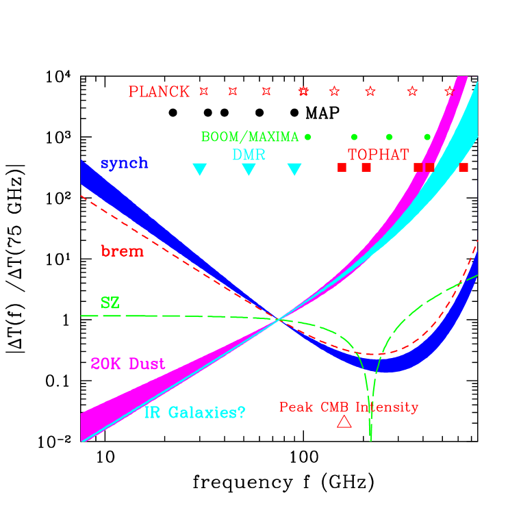
Figure 1.  : Foregrounds and secondary anisotropies depend differently on photon frequency, the key property for separating the components. Plotted is the frequency dependence of the effective thermodynamic temperature fluctuations, normalized to their values at 75 GHz. Thus the primary CMB fluctuations correspond to a horizontal line in this figure, synchrotron and bremsstrahlung dominate at low frequencies, dust at high. The bands represent a measure of our uncertainty in the appropriate foreground spectra. The highly distinctive shape for the Sunyaev-Zeldovich (SZ) effect is negative at low frequencies, positive at high. The actual level of contamination depends on the angular scale. The foreground emission is minimal around 90 GHz, not far from where the CMB intensity peaks. Detector frequencies for some notable experiments are denoted by the symbols at the top. Currently, detectors below 100 GHz are HEMTs, above are bolometers. Note the wide coverage planned for the Planck satellite which uses both.

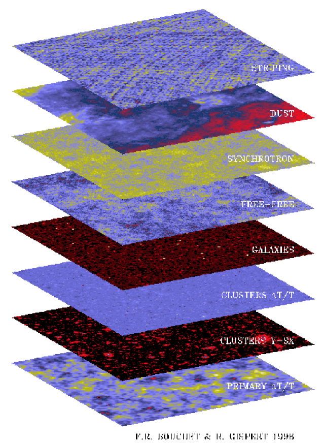
Figure 2.  : A schematic view by Bouchet and Gispert of many of the possible microwave foregrounds that need to be separated from the primary CMB anisotropy pattern shown in the $10^{\circ}$ map at the bottom. These include noise effects (striping), galactic foregrounds (dust, synchrotron and bremsstrahlung or free-free emission) as well as secondary anisotropies (extragalactic radio and infrared galaxies, CMB upscattering by hot gas in clusters – “clusters Y-SX,” and the Doppler effect arising from moving clusters – the kinetic SZ effect or “clusters $\Delta T/T$”). Each of these has a unique temperature pattern on the sky, and all but the kinetic SZ effect have a different spectral signature (Fig. 1).

1.2 Primary Theory and Current Data: We think we know how to calculate the primary signal in exquisite detail. The fluctuations are so small at the epoch of photon decoupling that linear perturbation theory is a superb approximation to the exact non-linear evolution equations. Intense theoretical work over three decades has put accurate calculations of this linear cosmological radiative transfer problem on a firm footing, and there are speedy, publicly available and widely used codes for evaluation of anisotropies in a wide variety of cosmological scenarios, e.g. “CMBfast” [1]. These have been further modified by many different groups to attack even more structure formation models.

The simplest and thus least baroque versions of inflation theory predict that the fluctuations from the quantum noise that give rise to structure form a Gaussian random field. Linearity implies that this translates into temperature anisotropy patterns that are drawn from a Gaussian random process and which can be characterized solely by their power spectrum. The emphasis is therefore on confronting the theory with the data in power spectrum space, as in Fig. 3. The panels show how the power spectrum ${\cal C}_{\ell}$ responds as various cosmological parameters are individually changed.

Until a few years ago, the emphasis was on fairly restricted parameter spaces, but now we consider spaces of much larger dimension. These are used for forecasts of how well proposed experiments can do, and for the first round of data from a sequence of high-precision experiments covering large areas of sky: ground-based single dishes and interferometers; balloons of short and long duration (LDBs, $\sim$ 10 days) and eventually of ultra-long duration (ULDBs, $\sim$ 100 days); NASA’s MAP satellite in 2001 and ESA’s Planck Surveyor in 2007. The lower right panel of Fig. 3 gives a forecast of how well we think that the two satellite experiments can do in determining $C_{\ell}$ if everything goes right. This rosy prognosis should be compared with the compressed bandpowers shown in the other panels estimated from all of the current data: DMR and some 19 other pre-conference “prior” experiments, TOCO [2], unveiled about the time of the conference, and four that appeared after the conference, the Boomerang flights (the LDB flight [3, 4] and its North America test flight [5]) the Maxima-I [6, 7] flight, the first results from CBI, the Cosmic Background Imager [8], and from DASI, the Degree Angular Scale Interferometer [9]. Although new methods have been applied to these data sets, much was in place and some algorithms were well tested on previous data, in particular DMR, SK95, MSAM and QMAP.

Although we sketch the current state of the art in CMB analysis in this paper, note that this is a very fast moving subject. A large number of researchers in a handful of groups are working on a broad range of issues, often as members of the experimental teams associated with the increasingly complex experiments. A snapshot of the state two years ago and references to the relevant papers was given in [33], but many advancements have been made since then. For example, the MAP plan for analysis is described in [40]. One issue that still needs to be addressed is that the strong simplifying assumptions of signal and noise Gaussianity cannot be correct in detail, and could yield misleading results.

1.3 Primary Parameter Sets for Gaussian Theories: A “minimal” inflation-motivated parameter set involves about a dozen parameters, e.g., $\{\omega_{b},\omega_{cdm}$, $\omega_{hdm},\omega_{er}$, $\Omega_{k},\Omega_{\Lambda}$, $\tau_{C}$, $\sigma_{8}\,,n_{s}$, $\tilde{r}_{t},n_{t}\}$. For many species we use $\omega_{j}\equiv\Omega_{j}{\rm h}^{2}$ rather than $\Omega_{j}$ since it directly gives the physical density of the particles rather than as a ratio to the critical density: thus, $\omega_{b}$ for baryons, $\omega_{cdm}$ for cold dark matter, $\omega_{hdm}$ for hot dark matter (massive but light neutrinos), and $\omega_{er}$ for relativistic particles present at decoupling (photons, very light neutrinos, and possibly weakly interacting products of late time particle decays). The total non-relativistic matter density is $\omega_{m}\equiv\omega_{hdm}+\omega_{cdm}+\omega_{b}$.

The curvature energy relative to the closure density is $\Omega_{k}\equiv 1-\Omega_{tot}$ and $\Omega_{\Lambda}$ is the energy relative to closure in the cosmological constant. $\Omega_{\Lambda}$ can also be interpreted as a vacuum energy, a sector which may be more complex and require more parameters. For example, a scalar field which dominates at late times, “quintessence”, has potentials and other interactions which must be set. A simple phenomenology of quintessence has added to $\Omega_{Q}$ an average equation of state pressure-to-density ratio $w_{Q}\equiv\bar{p}_{Q}/\bar{\rho}_{Q}$.

Another factor crucial for predicting the CMB anisotropies is $\tau_{C}$, the Compton depth to Thompson scattering from now back through the period when the universe was reionized by early starlight.

To characterize the initial fluctuations, amplitudes and tilts are required for the various fluctuation modes present. For adiabatic scalar perturbations, the tilt is $n_{s}$ and the amplitude is most appropriately the overall power in curvature fluctuations, but is often replaced by $\sigma_{8}^{2}$, a density bandpower on the scale of clusters of galaxies, $8{\,{\rm h}^{-1}~{}\rm Mpc}$. For tensor modes induced by gravity waves, the amplitude parameter is some measure of the ratio of gravity wave to scalar curvature power, $\tilde{r}_{t}$; usually a ratio of ${\cal C}_{\ell}$’s is used, e.g., at $\ell$=2 or 10. Inflation theories often give relationships between the tensor tilt $n_{t}$ and $\tilde{r}_{t}$ which can be used to reduce the parameter space e.g., [10]. Parameters for the amplitude and tilt of scalar isocurvature modes could also be added to the mix. The characterization of the modes present in the early universe by amplitude and tilt could be expanded to include parameters describing the change of the tilts with scale ($dn_{s}/d\ln k$), the change of that change, and so on. Relatively full functional freedom in $n_{s}(k)$ is possible in inflation models, and substantial freedom also exists for $n_{t}(k)$.

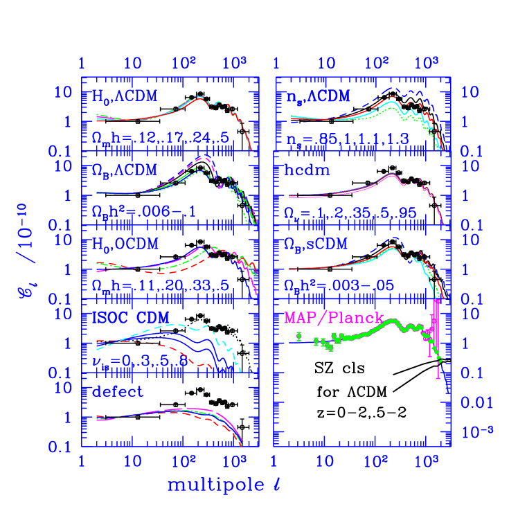
Figure 3.  : The ${\cal C}_{\ell}$ anisotropy bandpower data, including the recent balloon-borne and interferometry data, compressed to 13 bands using the methods of [14] are compared with various ${\cal C}_{\ell}$ model sequences, each for universes with age 13 Gyr (left to right): (1) untilted flat $\Lambda$CDM sequence with $H_{0}$ varying from 50 to 90, $\Omega_{\Lambda}$ from 0 to 0.87; (2) $n_{s}$ varying from 0.85 to 1.3 for an $H_{0}=70$ ($\Omega_{\Lambda}$=.66) $\Lambda$CDM model – dotted is 0.85 with gravity waves, next without, upper dashed is 1.25, showing visually why $n_{s}$ is found to be nearly unity; (3) $\Omega_{B}{\rm h}^{2}$ varying from 0.0063 to 0.10 for the $H_{0}$=70 $\Omega_{\Lambda}$=.66 $\Lambda$CDM model; (4) neutrino fractions $\Omega_{hdm}/\Omega_{m}$ varying from 0.1 to 0.95 for an $H_{0}$=50 $\Omega_{\Lambda}$=0 sequence with $\Omega_{m}$=1; (5) $H_{0}$ from 50 to 65, $\Omega_{k}$ from 0 to 0.84 for the untilted oCDM sequence, showing the strong $\ell$-shift of the acoustic peaks with $\Omega_{k}$; (6) $\Omega_{B}{\rm h}^{2}$ varying from 0.003 to 0.05 for the $H_{0}=50$ $\Omega_{\Lambda}$=0 sCDM model; (7) an isocurvature CDM sequence with positive isocurvature tilts ranging from 0 to 0.8; (9) sample defect ${\cal C}_{\ell}$’s for textures, etc. from [15] – cosmic string ${\cal C}_{\ell}$’s from [16] are similar and also do not fare well compared with the current data. The bottom right panel is extended to low values to show the magnitude of secondary fluctuations from the thermal SZ effect for the $\Lambda$CDM model. The kinematic SZ ${\cal C}_{\ell}$ is significantly lower. Dusty emission from early galaxies may lead to high signals, but the power is concentrated at higher $\ell$, with a weak tail because galaxies are correlated extending into the $\ell\mathrel{\hbox to0.0pt{\lower 3.0pt\hbox{$\mathchar 536\relax$}\hss}\raise 2.0pt\hbox{$\mathchar 316\relax$}}2000$ regime. Forecasts of how accurate ${\cal C}_{\ell}$ will be determined for an sCDM model from MAP (error bars growing above $\ell\sim 700$) and Planck (small errors down the ${\cal C}_{\ell}$ damping tail) are also shown.

1.4 Well and Poorly Determined Parameter Combinations: In Fig. 3, we compare the compressed bandpowers with ${\cal C}_{\ell}$ sequences as $\omega_{b}$, $\Omega_{tot}$, $\Omega_{\Lambda}$, $\omega_{hdm}$ and $n_{s}$ are individually varied. These show the discriminatory power of the current data. Fixing the age at 13 Gyr as we do here defines a specific relation between $\omega_{k}$, $\omega_{\Lambda}$ and $\omega_{m}$. From these figures, we expect that four can be determined reasonably well ($\omega_{b},\Omega_{tot},n_{s}$ and the overall amplitude). This is borne out in the full study with the real data, modulo parameter correlations which mean the best determined quantities are linear combinations of parameters, or parameter eigenmodes [12, 13, 10]. For example, it is actually a combination of $\Omega_{tot}$ and $\Omega_{\Lambda}$ which is well determined, but it happens to be $\Omega_{tot}$–dominated. Another orthogonal combination of the two will remain very poorly determined no matter how good the CMB data gets [12], an example of a near-degeneracy among cosmological parameters. Other near-degeneracy examples are less severe: e.g., $\Omega_{hdm}/(\Omega_{cdm}+\Omega_{hdm})$ is not well determined by current data, but could be by Planck.

Accompanying the idealized bandpower forecasts are predictions for how well the cosmological parameters in inflation models can be determined after integrating, i.e., marginalizing, the likelihood functions over all other parameters. In one exercise that allowed a mix of nine cosmological parameters to characterize the space of inflation-based theories (the 11 above with $\omega_{er}$ fixed and $n_{t}$ slaved to $\tilde{r}_{t}$), COBE was shown to determine one combination of them to better than 10% accuracy, LDBs and MAP could determine six, and Planck seven [13]. All currently planned LDBs could also get two combinations to 1% accuracy, MAP could get three, and Planck five. With the current data, one can forecast four to 10% accuracy, which is actually borne out in detailed computations with the data.

Two panels in Fig. 3 show what happens when two classes of pure isocurvature models are considered, one a Gaussian isocurvature CDM model with the spectral index allowed to tilt arbitrarily, another a set of non-Gaussian cosmic defect models. Neither fare well with the current data. Primary anisotropies in defect theories are more complicated to calculate because non-Gaussian patterns are created in the phase transitions which evolve in complex ways and which require large scale simulations. The non-Gaussianity means that the comparison with the data should be done more carefully, without the Gaussian assumption that goes into the bandpower estimations.

1.5 Current CMB and CMB+LSS Constraints: Although the purpose of this paper is to describe CMB analysis techniques, the comparison of the radically-compressed current bandpowers with the models in Fig. 3 invite a brief description of the results. Explicit numbers are those derived in [4] for the “minimal” inflation-motivated 7-parameter set for the combination of DMR and Boomerang, with a weak prior probability assumption on the Hubble parameter ($0.45<h<0.90$) and age of the Universe ($>10$ Gyr.) Including all other current CMB data as well gives very similar estimates and errors, reflecting the consistency between the older, less statistically significant data and the new experiments. (DMR+DASI numbers [9] are quite close to DMR+Boomerang numbers, since the spectra are similar. For a more complete description, see [32, 56, 65, 4, 9, 7].)

1.5.1 CMB-only Estimates: As the upper right panel of Fig. 3 suggests, the primordial spectral tilt $n_{s}$ is well determined using CMB data alone: $n_{s}$ = $0.97^{+.10}_{-.08}$. This is rather encouraging for the nearly scale invariant models preferred by inflation theory. The figure also shows that constraints on $\Omega_{\Lambda}$ will not be very good, but the strong dependence of the position of the acoustic peaks on $\Omega_{k}$ means that it is better restricted: $\Omega_{tot}\approx 1.02\pm 0.06$. The baryon abundance is also well determined, $\Omega_{b}h^{2}=0.022\pm 0.004$, near the $0.019\pm 0.002$ estimate from deuterium observations in quasar absorption line spectra combined with Big Bang Nucleosynthesis theory.

The isocurvature CDM models with tilt $n_{is}>0$ and the isocurvature defect models (e.g. strings and textures) [15, 16] shown in Fig. 3 clearly have more difficulty with the CMB bandpowers.

There is a region of the spectrum that nominally seems to be out of reach of CMB analysis, but is actually partly accessible because ultralong waves contribute gentle gradients to our CMB observables. For example, the size of compact spatial manifolds has been constrained; [66] find for flat equal-sided 3-tori, the inscribed radius must exceed $1.1\chi_{lss}$ from DMR at the $95\%$ confidence limit, where $\chi_{lss}$ is the distance to the last scattering surface. For asymmetric 1-tori, the constraint is weaker, $>0.7\chi_{lss}$, but still reasonably restrictive. It is also not as strong if the platonic-solid-like manifolds of compact hyperbolic topologies are considered, though the overall size of the manifold should as well be of order the last scattering surface radius to avoid conflict with the large scale power seen in the COBE maps [66].

1.5.2 CMB+LSS Estimates: We have always combined CMB and LSS data in our quest for viable models. For example, DMR normalization determines $\sigma_{8}$ to within 7%, and comparing with the $\sigma_{8}\sim 0.55\Omega_{m}^{-0.56}$ target value derived from cluster abundance observations severely constrains the cosmological parameters defining the models. This is further restricted when the possible variations in the spectral tilt allowed by the COBE data are constrained by the higher $\ell$ Boomerang data. More constrictions arise from galaxy-galaxy and cluster-cluster clustering observations: the shape of the linear density power spectrum must match the shape reconstructed from the data. In [32, 56, 65, 4], the LSS data were characterized by a simple shape parameter and $\sigma_{8}$, with distributions broad enough so that these prior probability choices would not be controversial, but encompass the ranges that almost all cosmologists would believe.

Using all of the current CMB data and the LSS priors, [4] got $H_{0}=56\pm 9$, $\Omega_{\Lambda}=0.55\pm 0.09$, with $n_{s}$, $\Omega_{tot}$ and $\Omega_{b}h^{2}$ virtually unchanged from the CMB-only result. Apart from the significant $\Omega_{\Lambda}$ detection, the dark matter is also strongly constrained, $\Omega_{cdm}h^{2}=0.13^{+.03}_{-.02}$. Restricting $\Omega_{tot}$ to be unity as in the usual inflation models, with CMB+LSS, $\Omega_{b}h^{2}=0.021\pm 0.003$, $\Omega_{cdm}h^{2}=0.13\pm 0.01$, $\Omega_{\Lambda}=0.62\pm 0.07$ and $n_{s}$ = $0.98^{+.10}_{-.07}$. If the equation of state of the dark energy is allowed to vary, $w_{Q}<-0.3$ is obtained, becoming substantially more restrictive when supernova information is folded in, $w_{Q}<-0.7$ at 2 $\sigma$ [65].

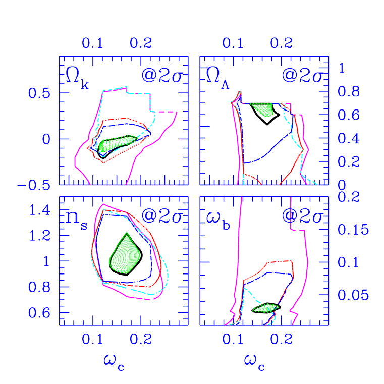
Figure 4.  : This figure from [65] shows 2-$\sigma$ likelihood contours for the dark matter density $\omega_{c}=\Omega_{cdm}{\rm h}^{2}$ and $\{\Omega_{k},\Omega_{\Lambda},n_{s},\omega_{b}\}$ for the LSS prior combined with weak limits on $H_{0}$ (45-90) and cosmological age ($>10$ Gyr), and the following CMB experimental combinations: DMR (short-dash); the “April 99” data (short-dash long-dash); TOCO+4.99 data (dot short-dash); Boomerang-NA+TOCO+4.99 data (dot long-dash, termed “prior-CMB”); Boomerang-LDB + Maxima-1 + Boomerang-NA + TOCO + 4.99 data (heavy solid, all-CMB). These $2\sigma$ lines tend to go from outside to inside as more CMB experiments are added. The smallest 2-$\sigma$ region (dotted and interior) shows SN1+LSS+all-CMB, when SNI data is added. For the $\Omega_{\Lambda}$, $n_{s}$ and $\omega_{b}$ plots, $\Omega_{tot}$=1 has been assumed, but the values do not change that much if $\Omega_{tot}$ floats. The main movement with the most recent data [4] is that $\omega_{c}$ localizes more around 0.13 in all panels, and the $\omega_{b}$ contour in the lower right panel migrates downward a bit to be in better agreement with the Big Bang nucleosynthesis result.

Fig. 4 gives a visual perspective from [65] on how the parameter estimations for the adiabatic models evolved as more CMB data were added (but with always the LSS prior included for this figure). With just the COBE-DMR+LSS data, the 2-$\sigma$ contours were already localized in $\Omega_{cdm}h^{2}$. Without LSS, it took the addition of Maxima-1 before it began to localize. $\Omega_{k}$ localized near zero when TOCO was added to the April 99 data, more so when Boomerang-NA was added, and much more so when Boomerang-LDB and Maxima-1 were added. Some $n_{s}$ localization occurred with just “prior-CMB” data. $\Omega_{b}h^{2}$ really focussed in with Boomerang-LDB and Maxima-1, as did $\Omega_{\Lambda}$. If only DMR plus the most recent Boomerang results [4] to $\ell=600$ are used (the limit in [3]), the plot is rather similar. However, when all recent Boomerang [4] results to $\ell=1000$ are used, the inner contour in the $\Omega_{cdm}h^{2}$ direction sharpens up in all panels, and the $\Omega_{b}h^{2}$ contour lowers to be in the good agreement with the big bang nucleosynthesis result indicated above.

2 Computing Non-Gaussian Secondary Signals: the SZ Example

The secondary fluctuations involve nonlinear processes, and the full panoply of $N$-body and gas-dynamical cosmological simulation techniques are being used to study them. It is realistic to hope that the thermal and kinetic Sunyaev-Zeldovich effects can be understood statistically this way with sufficient accuracy for CMB analysis, and this is the main example used in this section. On the other hand, star-bursting galaxies will be quite difficult to understand from simulations alone, but CMB analysis will be greatly aided by their point-source character for most experimental resolutions. Galactic foregrounds, however, cannot be “solved” by hydro calculations.

2.1 Hydrodynamical Calculations: The Santa Barbara test [17] compared simulations of an individual cluster of $10^{15}{\,M_{\odot}}$ done with a variety of hydrodynamical and N-body techniques, in particular grid-based Eulerian methods and both grid-based and smooth particle (SPH) Lagrangian methods. (Eulerian grids are fixed in comoving space, Lagrangian grids adapt to the density of the flow.) Fig 5 shows this cluster, computed with the treePM-SPH code of Wadsley and Bond [19, 20], seen at the present in weak lensing, SZ and X-rays, at contour thresholds designed to represent potentially observable levels. For a review of the great strides made in SZ experimental methods and results on individual clusters up to 1998 see [18].

Another hydrodynamical example, the simulation of a supercluster [20, 21] using the treePM-SPH code, is used to illustrate the computational challenges once we extend beyond individual cluster simulations. Fig. 7 shows thermal SZ maps of the supercluster at redshift $z=0.5.$ The computation evolved from redshift $z=30$ to the present a high resolution 104 Mpc diameter patch with $100^{3}/2$ gas and $100^{3}/2$ dark matter particles, surrounded by gas and dark particles with 8 times the mass to 166 Mpc, in turn surrounded by “tidal” particles with 64 times the mass to 266 Mpc.

There were a total of 1.6 million particles including the medium and low resolution regions, but much larger simulations are possible in this era of massive parallelization. For example, a parallel tree-SPH code (“gasoline”), with timesteps that can vary from particle to particle, can routinely do $256^{3}$ gas and $256^{3}$ dark matter simulations, and even $512^{3}$ simulations on relatively modest ($<100$ processor) BEOWULF systems [31].

The treePM technique is a fast, flexible method for solving gravity and can accurately treat free boundary conditions. The SPH part of the code includes photoionization as well as shock heating and cooling with abundances in chemical (but not thermal) equilibrium, incorporating all radiative and collisional processes. The species considered were H, H⁺, He, He⁺, He⁺⁺ and e^-. The extra cooling associated with heavy elements injected into the intracluster media during galactic evolution was ignored, but so was the feedback on the medium from energy injected from galactic supernovae: the computation does not have high enough spatial resolution to calculate galaxy collapse.

We now describe some aspects of simulation design for the supercluster simulation [20, 21] which are also relevant for the larger parallel calculations. One first decides on the mass resolution to achieve, which is set by the lattice spacing of particles on an initial high resolution grid, $a_{L}$, chosen to be $\sim 1{\rm~{}Mpc}$ comoving to ensure that there will be adequate waves to form the target objects, in this case clusters. Next one needs to determine the spatial resolution of the gas and of the gravitational forces, preferably highly linked. In Lagrangian codes like treePM-SPH, this varies considerably, being very high in cluster cores, moderate in filaments, and not that good in voids. Since accurate calculations of the cluster cores were a target, resolution better than $\sim 40{\rm~{}kpc}$ was desired. The best resolution obtained was about $15{\rm~{}kpc}$. Given $a_{L}$, the size of the high resolution part of the simulation volume is determined by CPU limitations on the number of particles that can be run in the desired time. This means the high resolution volume may distort considerably during the simulation. To combat this, progressively lower resolution layers were added to ensure accurate large scale tides/shearing fields operated on the high resolution patch. For the calculations shown, the high resolution region (grid spacing $a_{L}$, $100^{3}$ sphere) sits within a medium resolution region ($2\,a_{L}$, $80^{3}$), and in turn within a low resolution region ($4\,a_{L}$, $64^{3}$). The mean external tide on the entire patch is linearly evolved and applied during the calculation.

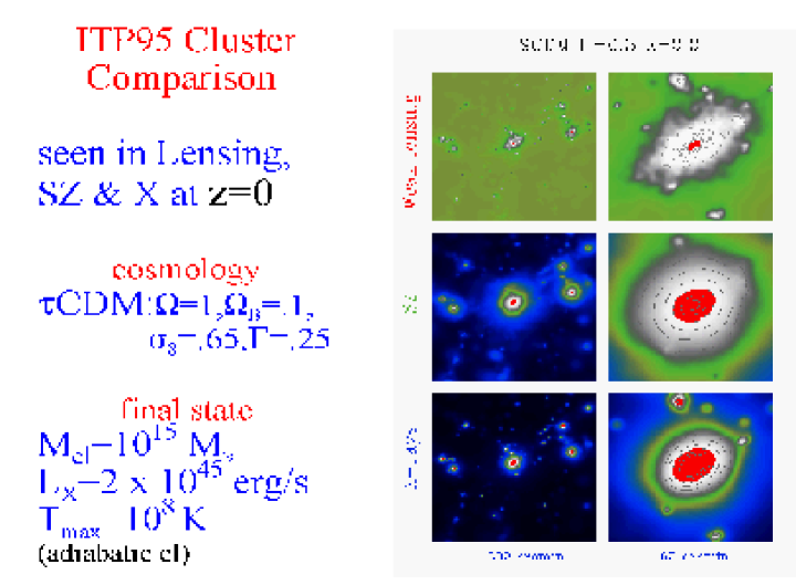
Figure 5.  : SZ maps for the ITP comparison cluster seen at $z=0$ subtending the angles shown. The observing wavelength was taken to be in the Rayleigh-Jeans region of the spectrum, so $\Delta T/T=-2y$ here. The core dark regions interior to the white areas are above $32\times 10^{-6}$; the dark contours surrounding the white are at $2\times 10^{-6}$, levels now accessible to ground-based instrumentation. At higher redshift, gaseous filaments bridge the subclusters which merge to make the final state. Even the far-field outskirts of these subclusters is observable, but precision below $10^{-6}$ would be needed to probe well the filaments. (See also Fig. 7.)

2.2 Non-Gaussian Source Model: It is clear from Figs. 6 and 7 that the dominant signals are quite patchy if one is interested in amplitudes above a few $\mu K$. This has the disadvantage for analysis that non-Gaussian aspects of the predicted patterns are fundamental, and an infinite hierarchy of connected $N$-point spectra beyond the 2-point spectrum $C_{\ell}$ are required to specify them (as for defect models). However, it also seems reasonable that we could represent the results in terms of extended emission from localized sources. This concentration of power is characteristic of many types of secondary signals. Indeed some, such as radiation from dusty star-burst regions in galaxies, can be treated as point sources since they are much smaller than the observational resolution of most CMB experiments. However, highly accurate emission from dusty galaxies is too difficult to calculate from first principles, and statistical models of their distribution must be guided by observations.

Extended and point source models for the temperature fluctuations express the signal as a projection along the line-of-sight of a 3D random field, ${\cal G}({\bf r},t)$, which is the convolution of profiles $g({\bf r}|{\cal C},t)$ surrounding objects of some class ${\cal C}$, with the comoving number density $n_{{\cal C}*}({\bf r},t)$ defining a point process for those objects [10, 28]. In [28, 29], the points were referred to as “shots”, from shot-noise, although of course continuous clustering of the shots as well as their uncorrelated Poissonian self-correlation has to be included. Simple derivations for the form of ${\cal G}({\bf r},t)$ and $g$ and the relation of the 2D power spectrum ${\cal C}_{\ell}$ to the 3D power spectrum of the ${\cal G}$ (and hence of $n_{{\cal C}*}$) are given in [10].

For dusty star-burst regions, the shots are galaxies and the profile $g$ involves the dust density and temperature [28, 29], while for the SZ effect, the dominant emission comes from clusters and groups and the profile $g$ is a constant times the pressure [28, 10, 30].

Various attempts have been made to use hydrodynamical codes to do an entire region up to $z=2$ or so. However, it should be clear from the discussion of the numerical setup that approximations are always needed to do this. One approach was to calculate the full pressure power spectrum from a single simulation, ${\langle|\widetilde{{\cal G}}(k,t)|^{2}\rangle}$, and appropriately project it to determine the SZ ${\cal C}_{\ell}$ [22, 23]. A more ambitious approach was to tile the space with boxes out to some redshift [24, 25, 26, 27, 31], but because of computer limitations and resolution requirements, the boxes were relatively small and computationally expensive. To make predictions, tricks were required, e.g., “observing’ translated and rotated versions of the few simulated boxes at many different output redshifts.

   

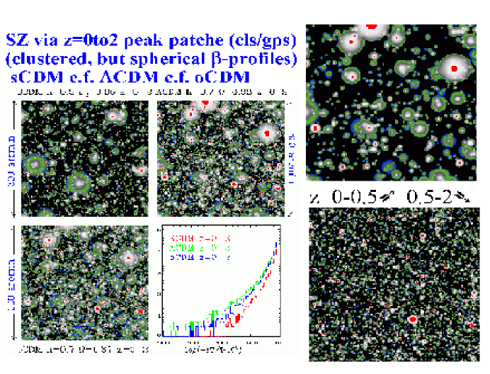
Figure 6.  : SZ maps derived from spherical presure-profiles imposed upon halos identified up to $z$=2 with the peak-patch method, for three cluster-normalized cosmological models. The observing wavelength and contours are the same as in Fig. 5. The histograms show $\Lambda$CDM, $o$CDM and sCDM can be clearly differentiated. Blank field SZ surveys using interferometers and bolometer experiments promise to revolutionize our approach to the cluster system, especially at $z\mathrel{\hbox to0.0pt{\lower 3.0pt\hbox{$\mathchar 536\relax$}\hss}\raise 2.0pt\hbox{$\mathchar 318\relax$}}0.5$. The contributions from clusters below and above this redshift are shown on the right for the $\Lambda$CDM model.

2.3 The Shots and their Profiles: The shot model provides a way forward semi-analytically, by laying down pressure profiles around a catalogue of halos. The halos and their properties could be computed with $N$-body-only simulations using much larger boxes than those required for hydro. Another approach is to use “peak-patches”, a method for identifying halos in the initial conditions of calculations which has been shown to be accurate for clusters [30]. For this approach, the entire space can be tiled with contiguous boxes that are smoothly joined, and have all the required long wavelength power to treat the really rare halo concentrations, or “super-duper-clusters”, that can appear.

What to do for the pressure profiles, $p({\bf r}|{\cal C},t)$, is of course debatable. One strategy is to use profiles calculated from hydro simulations, but what has invariably been done is even simpler: pressure profiles scaled by bulk halo properties of the observed form derived from low redshift X-ray cluster data (and extrapolated to the more poorly known high redshift regime). For example, adopting a spherically symmetric isothermal “beta” profile is common: $p({\bf r}|{\cal C},t)=p_{c}(1+r^{2}/r_{core*}^{2})^{-3\beta/2}\vartheta(R_{{\cal C}*}-r)$, where $p_{c}$ is the central pressure, $r_{core*}$ is a core radius, and $R_{{\cal C}*}$ is an outer truncation radius exterior to which the local pressure contribution is taken to be zero, and interior to which $\vartheta$ is unity. The radius $r$ here is comoving and the $*$ subscript denotes comoving radii. $\beta\approx 2/3$ is a reasonable fit to the X-ray data.

This rapid semi-analytic peak-patch method for simulating clusters using isothermal beta-profiles was used in the construction of the two SZ layers (thermal and kinetic) of the sandwich in Fig. 2. The panels of Fig 6 show peak-patch-derived SZ maps for three cosmologies, and the lower right corner shows the distribution of $\Delta T/T$ in pixels, with its non-Gaussian distinct tails. The right two panels contrast the contribution for the $\Lambda$CDM example of clusters below $z=0.5$ with those above. The top panel of Fig. 7 shows the $\Lambda$CDM example with a filter scale appropriate for the Planck satellite resolution and with an ideal resolution for the cluster system, below two arcminutes, which interferometers and large single dishes can achieve. However, interferometers typically filter the low $\ell$, losing large scale power. The lower panel of Fig. 3 shows the SZ ${\cal C}_{\ell}$ spectrum derived for the flat $\Lambda$CDM simulation shown, contrasting the contributions from clusters and groups above $z=0.5$ with all of them. Both Poissonian and clustering contributions are included, since the simulation has them.

The power is not distributed in a democratic fashion as it is for Gaussian theories, but is concentrated in cold spots below 218 GHz, and in hot spots at higher frequencies. Thus, the naive visual comparison with bandpowers derived using a Gaussian assumption about the distribution of power is misleading.

The assumption that the SZ effect is dominated by the high pressure regions associated with clusters and groups of galaxies, with only weak modifications coming from the intercluster medium, is borne out visually in the supercluster simulation. The emission from the gas in filaments outside of the groups and poor clusters that reside in them is weak, below observable levels. What we can also see, however, is that an anisotropic pressure distribution is expected, with elongation along the filament directions, inviting improvements over spherical approximations.

   

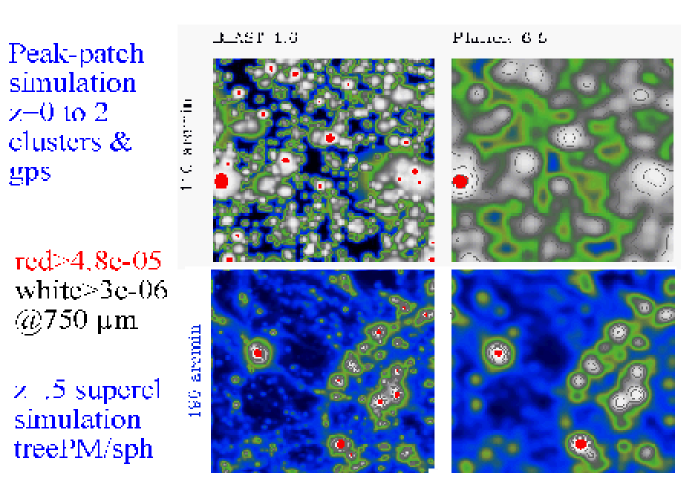
Figure 7.  : SZ maps subtending the angles shown for peak patches (above) and a single supercluster region seen at redshift 0.5. The core dark regions interior to the white areas are above $48\times 10^{-6}$, and the dark contours surrounding the white are at $3\times 10^{-6}$ at 750$\mu m$, levels that can be achieved with blank field SZ bolometer experiments. Filamentary bridges between the clusters are typically below $10^{-6}$, but the far-field of clusters can be probed. The bottom left panel passes the supercluster region at $z=1$ in the right panel through a simulated 30 GHz HEMT-based interferometer with the indicated characteristics.

To properly analyze the SZ effect in ambient fields, having fast Monte Carlo simulation methods along the lines developed here is clearly essential. That does not take away from the challenge of how best to do the analysis of such distinctly non-Gaussian signals, which consist of extended rather than point-like sources. Even with relatively small beams, these will be somewhat confused by overlapping sources. At least with the cluster system, we may hope to model the individual elements with hydrodynamical simulations. For other secondary sources such as dusty galaxies, a priori theoretical models are not really feasible, and the properties of the sources will have to be derived from the observations. At least in some of those cases, for typical beam sizes, the emission can be treated as from point sources.

2.4 Foreground Complications: The foreground signals from the interstellar medium are also non-Gaussian, but are not well-modelled by extended sources, since their emission power spectrum ${\cal C}_{\ell}$ has been shown to rise to lower $\ell$; further, no simplifications such as statistical isotropy apply. Direct hydrodynamical studies may increase our understanding of the ISM, but will not be able to provide strong guidance on statistical comparisons with data. The use of other data sets will clearly play a strong role in the final analysis; e.g., templates from the IRAS+DIRBE data is useful for modelling the distribution of shorter wavelength dust radiation. Exactly what to do for the analysis of foregrounds is under intense study and some current ideas are described in § 3.

3 Acting on the Data

The data comes in as raw timestreams, which must be cleaned of cosmic rays, obvious sectors of bad data, and other contaminants. Encoded in it are the sky and noise, as well as unwanted instrument, atmospheric and other residual signals. The pointing matrix identifies time-bits to a chosen pixel basis and allows the spatial signal to be separated from the noise; the resulting map completely represents the data if the pixelization is fine enough relative to the experiment’s beam. At one time, the cosmology was drawn from the maps, perhaps using new bases beyond the spatial pixel ones, and possibly truncated to compress the data into more manageable chunks (e.g., using signal-to-noise eigenmodes to get rid of informationless noisy components of the map, [11]).

The statistical distribution of various operators on the pixelized data can be estimated from the map. In particular, the power spectrum ${\cal C}_{\ell}$ represents a radical compression of the data, but of course is no longer a complete representation of the map. However, under the assumption that the sky maps only contain Gaussian signals characterized by an isotropic power spectrum, this is a complete representation of the statistical information in the map when the binning of the bandpowers is fine enough. For such Gaussian theories, such as those usually arising in inflation, cosmological parameters can be quickly estimated directly from the power spectrum. The radical compression has allowed millions of theoretical models to be confronted with the data in the large cosmological parameter spaces described above, e.g., [32], a situation infeasible if full statistical confrontation of all the models with the maps was required.

Basic aspects of the Boomerang, Maxima, DASI and CBI pipelines are described in [33], [35, 37, 4, 38], [36, 39], [9] and [8]. Pipelines were also developed for DMR and for QMAP. The MAP pipeline as currently envisaged is described in [40]. The Planck pipeline is still very much under discussion and development, complicated by the necessity of delivering high precision component maps and derived parameters from such a huge volume of data.

3.1 Bayesian Chains: The data analysis pipeline can be viewed as a Bayesian likelihood chain:

$${\cal P}(parameters|data,\ theoretical\ framework)$$

$$={\cal P}(data\ timestreams|maps,\ noise)$$

$$\ \ \otimes{\cal P}(noise|noise-obs)$$

$$\quad\otimes{\cal P}(maps|signals)$$

$$\qquad\otimes{\cal P}(signals|parameters)$$

$$\ \qquad\otimes{\cal P}(parameters|prior\ knowledge)$$

$$\ \ \qquad\otimes[1/{\cal P}(data|theoretical\ framework)]$$ (1)

Each conditional probability in the unravelling of the chain is very complex in full generality. This means the exact statistical problem is probably not solvable, and only applying simplifying approximations to sections of the chain have made it tractable. Of particular widespread use has been the assumption that both noise and signals are Gaussian-distributed; others are being explored, especially by Monte Carlo means, but much remains to be done for us to attain the high precision levels that have been forecast.

We now describe the various terms, beginning with the last two. The priors ${\cal P}(parameters|prior\ knowledge)$ for the cosmological parameters are often taken to be uniform, but can represent information from other experiments, e.g., LSS observations, prior CMB experiments, age or $H_{0}$ constraints. The hope is that the new information from the rest of the probability chain will be so concentrated that the precise nature of the prior choice will not matter very much. As we have seen, prior information from non-CMB experiments is crucial, even given the most ideal CMB experiment, in order to break near-degeneracies among cosmological parameters.

The quantity ${\cal P}(data|theoretical\ framework)$ is an overall normalization. It can address whether the overall theory is crazy as an explanation of the data. It has some characteristics in common with goodness-of-fit concepts in “frequentist” probability analysis.

We often refer to entropies ${\cal S}\equiv\ln{\cal P}$ in the Gibbs sense so the Bayesian chain involves a sum of the individual conditional entropies that make up the whole.

3.2 Signal/noise separation: The information comes in the form of a discretized timestream, with $d_{ct}$ as the data for the bit of time $t$ in frequency channel $c$, and a pointing vector on the sky, ${\hat{q}}_{c}(t)$. The sky is gridded into pixels, and these are used to define signal maps which are functions of direction and frequency. We denote these by $\Delta_{cp}$, for the signal at pixel $p$ and frequency channel $c$. The pointing matrix, $P_{ctp}$, is an operator mapping time-bit $t$ to pixel $p$ with some weight. The difference $d-P\Delta$ is the noise, $\eta$, plus further residuals ${\cal R}$, which may be sky-based or experimental systematics. The probability of a given timestream can be written as

$${\cal P}(d|\Delta,\eta,P_{ctp})=\prod_{ct}\delta\big{(}d_{ct}-(\sum_{p}P_{ctp}\Delta_{cp}+{\cal R}_{ct}+\eta_{ct})\big{)}.$$ (2)

3.2.1 Map-making: Map-making for a given channel involves using just the information encoded in $d$ and $P$ to separate what is sky signal (and residuals) from what is noise, i.e., the construction of ${\cal P}(\Delta|d)$.

The pointing matrix is a projection operator, with many more time-bits than pixels. The simplest example for $P_{ctp}$ is the characteristic set function for the pixel $\chi_{p}({\hat{q}}_{c}(t))$ (one inside the pixel, zero outside). For a chopping experiment such as MAP, the two pixels where the two beams are pointing (separated by $141^{\circ}$) are coupled at a given time-bit. There are also choices to be made about scattering the information in the timestream among pixels. For example, one can include the beam in $\Delta$ or in $P$. At the moment the former is preferred, but there are good arguments for the latter if the beam changes in time (e.g., asymmetric beams with rotations). In that case, $\chi_{p}({\hat{q}}_{c}(t))$ is replaced by $A_{p}{\cal B}({\hat{q}}_{p}-{\hat{q}}_{c}(t))$, where ${\cal B}$ is the beam function and $A_{p}$ is the pixel area, and the derived signal $\Delta_{cp}$ does not have the beam function convolved with it as it does in the “top hat” $\chi_{p}$ case. Of course, any other function normalized to the pixel area upon integration can be used, e.g., approximations to the beam which might not contain all sidelobe information. As long as the signals are appropriately convolved, and the pixelization choices are fine enough, the results should be identical. Pointing uncertainty further complicates the simplicity of $P$.

In map-making, there is an implicit assumption on the prior probability of the map, ${\cal P}(\Delta|prior)$, that it is uniform so any value is a priori possible. The map distribution should involve integration over all possible noise distributions; in practice, only the measured noise is used, which delivers the maximum likelihood map $\overline{\Delta}_{cp}$ and a pixel noise correlation $C_{N,cpc^{\prime}p^{\prime}}$, allowing for possible channel-channel correlations in the noise.

For many previous experiments, one could just compute the average $\overline{\Delta}$ and variance $C_{N}$ of the measured $d$’s contribution to each pixel, relying on the central limit theorem to ensure a Gaussian-distribution. However, these “naive maps”, described below in more detail, also relied on an implicit assumption, namely that $\eta$ was uncorrelated from time-bit to time-bit, which is not correct with the $1/f$ noise in detectors. The noise was also often so strong compared with the signal that the latter could be ignored in solving for $\Delta_{cp}$; this is no longer the case.

So far it has been essentially universal to assume that $\eta$ is Gaussian-distributed stationary noise with noise power $w^{-1}(\omega)$ a smooth function. Thus, the noise is completely specified by its covariance $c_{n,ct,c^{\prime}t^{\prime}}\equiv{\cal S}[\langle\eta_{ct}\eta_{c^{\prime}t^{\prime}}\rangle]$, which is assumed to be a function of $t-t^{\prime}$, hence diagonal in the time frequencies $\omega$. Here, ${\cal S}$ denotes the smoothing operation. Drifts and non-Gaussian elements can be included with timestream filtering and in the catch-all residual ${\cal R}$ using time templates (see below). Ignoring ${\cal R}$ for the moment, the probability of the time-ordered data given a map and noise-power $w^{-1}$, ${\cal P}(d|\Delta,w)$, is just a Gaussian:

$${\cal P}(d|\Delta,w) = \exp[-(d-P\Delta)^{\dagger}w(d-P\Delta)/2]/\{(2\pi)^{N_{tbits}/2}\sqrt{{\rm det}(w^{-1})}\}$$ (3)

$$= \exp[-(\overline{\Delta}-\Delta)^{\dagger}W_{N}(\overline{\Delta}-\Delta)/2]/\{(2\pi)^{N_{pix}/2}\sqrt{{\rm det}(W_{N}^{-1})}\}$$

$$\times\exp[-\bar{\eta}^{\dagger}\widetilde{w}\bar{\eta}/2]/\{(2\pi)^{(N_{tbits}-N_{pix})/2}\sqrt{{\rm det}(\widetilde{w}^{-1})}\},$$

$$W_{N}\overline{\Delta}=P^{\dagger}wd,\qquad\qquad\,\,W_{N}\equiv P^{\dagger}wP\equiv C_{N}^{-1}={\langle nn^{\dagger}\rangle}^{-1},$$ (4)

$$n\equiv\overline{\Delta}-\Delta=C_{N}P^{\dagger}w\eta,\qquad\qquad\qquad\bar{\eta}\equiv{\langle\eta|d\rangle}=d-P\overline{\Delta},$$

$$\widetilde{w}=w(1-P(P^{\dagger}wP)^{-1}P^{\dagger}w),\qquad\qquad\qquad\qquad P^{\dagger}w\bar{\eta}=0.$$ (5)

The maximum likelihood solution for $w(\omega)$ is $({\cal S}[|{\rm FT}(d-P\overline{\Delta})|^{2}])^{-1}$, where FT denotes the Fourier transform operator. Note that the $\bar{\eta}$ noise term is multiplied by a projector which is perpendicular to the spatial sector; i.e., $C_{N}P^{\dagger}w\bar{\eta}$=0. The first Gaussian in eq.(3) is ${\cal P}(\overline{\Delta}|\Delta)$. We can interpret it as the integration over the spatial Gaussian random noise field $n$ defined in eq.(4) of the product of ${\cal P}(\overline{\Delta}|\Delta,n)=\delta(\overline{\Delta}-(\Delta+n))$ and the distribution of $n$, $\exp[-n^{\dagger}C_{N}^{-1}n/2]/[(2\pi)^{N_{pix}/2}[{\rm det}C_{N}]^{1/2}]$ .

3.2.2 General cf. Optimal Maps: Any linear operation from timestream to generalized pixels, $\overline{\Delta}^{({\cal M})}={\cal M}^{\dagger}d$ defines a map, albeit not an optimal one as for the maximum likelihood solution eq.(4). The map-noise $n^{({\cal M})}\equiv\overline{\Delta}^{(M)}-{\Delta}^{(M)}$ has a correlation matrix $C^{({\cal M})}_{N}={\cal M}^{\dagger}w^{-1}{\cal M}$. Here the relation of the true sky signal seen in the ${\cal M}$-filter-space to the “optimal map” signal $\Delta$ is ${\Delta}^{(M)}={\cal M}^{\dagger}P\Delta$. Of special interest are therefore classes of operators ${\cal M}$ for which ${\cal M}^{\dagger}P=P^{\dagger}{\cal M}$ is a projector, i.e., self-adjoint and equal to its square. For example, ${\cal M}^{\dagger}=(P^{\dagger}w_{*}P)^{-1}P^{\dagger}w_{*}$ satisfies ${\cal M}^{\dagger}P=I$, the identity, for any $w_{*}$ provided $(P^{\dagger}w_{*}P)$ is invertible. The price one pays for such a non-optimal map is enhanced noise, with noise-weight matrix $W_{N}^{({\cal M})}=(P^{\dagger}w_{*}P)(P^{\dagger}w_{*}w^{-1}w_{*}P)^{-1}(P^{\dagger}w_{*}P)$ which has maximum eigenvalues if $w_{*}=w$, but is otherwise “less weighty”.

An interesting example is when $w_{*}$ is taken to be a constant and $P_{tp}$ is zero or one depending if the pointing at a time-bit $t$ lies within the pixel $p$ or not; in that case $P^{\dagger}P$ just counts the number of time-bits that fall into each pixel, and $\overline{\Delta}^{({\cal M})}$ is just the average of the anisotropies over these. If we use $\eta_{t}\eta_{t^{\prime}}$ in place of its smoothed version $w^{-1}$, the noise matrix just counts the variance in the amplitudes of the pixel hits about the mean. For this reason, $(P^{\dagger}P)^{-1}P^{\dagger}d$ is called a “naive map” [4]. For other cases, computing the error matrix may not be simple if $w$ is not known.

For the full maximum likelihood map, even with stationarity, the convolution of $w$ with $d$ appears to be an $O(N_{tbits}^{2})$ operation, but it is really $O(N_{tbits})$ because $w(t-t^{\prime})$ generally goes nearly to zero for $t-t^{\prime}\gg 0$. Similarly, the multiplication of the pointing matrix is also $O(N_{tbits})$ because of its sparseness. Thus, we can reduce the timestream data to an estimate of the map and its weight matrix in only $O(N_{pix}^{2})$ operations.

3.2.3 Iterative Map-making Solutions: An iterative method [35] has proved quite effective to solve this: the map on iteration $j+1$ is estimated from $W_{*}\Delta_{(j+1)}=W_{*}\Delta_{(j)}+P^{\dagger}w_{(j)}\eta_{(j)}$, where the noise and noise power on iteration $j$ are determined from $\eta_{(j)}=d-P\Delta_{(j)}$, $w_{(j)}^{-1}(\omega)={\cal S}[|FT(\eta_{(j)})|^{2}(\omega)]$. Here $W_{*}\equiv P^{\dagger}w_{*}P$ is a matrix chosen to be easy to invert: e.g., a constant $w_{*}$ was used for Boomerang [35]. As the maps converge, the noise orthogonality condition holds, so the solution is the correct one. What $w(\omega)$ looks like is white noise at high temporal $\omega$, crashing to zero because of $1/f$ noise in the instruments and time-filtering. These low frequencies correspond to large spatial scales, and the iteration converges slowly there, inviting multigrid speedup of the algorithm, which is now being implemented [37]. The final $\overline{\Delta}$ and $C_{N}$ are computed using $d$ and the converged $w_{(j)}$ in eq.(4). In some instances, we can work directly with $W_{N}\overline{\Delta}$ and $W_{N}$ rather than $\overline{\Delta}$ and $C_{N}$, avoiding the costly $O(N_{pix}^{3})$ inversion. If sections of the map are cut out after $W_{N}$ determination, through a projector $\chi_{cut}$ which is zero outside and one inside the cut, the cut weight matrix is $(\chi_{cut}W_{N}^{-1}\chi_{cut})^{-1}$. This corresponds to integration over all possible values of the now unobserved $\overline{\Delta}$’s outside of the cut, which increases the errors on the regions inside because of the correlation. Unfortunately, two matrix inversions are required, and the first one is potentially quite large even if the cut is severe.

Hinshaw et al. [40] describe the current pipeline for MAP. To a good approximation the MAP noise is white, so $w_{(j)}=w_{*}$ can drop out, and the critical element is computation of $P^{\dagger}P$, which is more complex than counting pixel-hits because MAP is a difference experiment. The MAP team choose $W_{*}$ to be $diag(P^{\dagger}w_{*}P)$, but otherwise use the same iterative algorithm.

Since $P$ is all that differentiates signal from noise in the timestream, it is essential that it be sufficiently complex; in practice this means many cross linkages among pixels in the scan strategy. This is because there are random long term drifts in the instruments that make it hard to measure the absolute value of temperature on a pixel, though temperature differences along the path of the beam can be measured quite well because the drifts are small on short time scales. If there are not sufficient cross-links, the maps are striped along the directions of the scan pattern, and the weight matrix $W_{N}$ has to be called upon to demonstrate that these features are not part of the true sky signal we are searching for. The rapid on-board differencing for MAP effectively eliminates this.

3.3 Pixelization: Pixels are any discrete basis that give a complete representation of the data. Square top-hat functions tiling the space in a grid quite a bit smaller than the beam size were the norm in the past. As the size of the data increased, more elaborate hierarchical schemes were needed. For COBE, the Quadrilateralized Spherical Cube was used: the sky was broken into six base pixels corresponding to faces of a cube. Higher resolution pixels were created by dividing each pixel into four smaller pixels of approximately equal area, in a tree with pixels that are physically close having their data stored close to each other. There are (quite) small errors associated with the projections of the sphere onto the faces. At resolution $r$, there are $6\times 2^{2(r-1)}$ pixels. The COBE data came with resolution $r=6$, 6144 pixels of size $2.6^{\circ}$, and we sometimes use resolution 5, still safely smaller than the $7^{\circ}$ beam.

For large sky coverage, it is beneficial to have a pixelization which is azimuthal, with many pixels sharing a common latitude, to facilitate fast spherical harmonic transforms (FSHTs) [41] between the pixel space, where the data and inverse noise matrix are simply defined, and multipole space, where the theories are often simple to describe. The FSHT operation count is a ${\cal O}(N_{pix}^{3/2})$ operations, with ${\cal O}(N_{pix}\ln N_{pix}^{2})$ potentially possible to achieve. HEALPix[42] is an example which has been adopted for Boomerang, MAP and Planck: it has a rhombic dodecahedron as its fundamental base, which can be divided hierarchically while remaining azimuthal. There is also an extensive software package that accompanies it to allow manipulations. See also [43] for the alternative hierarchical “igloo” choice, with many HEALPix features, and some other advantages.

In some cases generalized pixels are used, involving direct projection of the data onto spatially-extended mode functions. The first extensive use of this was for the SK95 dataset. Signal-to-noise eigenfunctions used in data compression for COBE and SK95 are another example [11, 14]. Direct projection onto pixels in wavenumber space, with the mode functions being discrete Fourier transform waves, also form a fine alternative basis. Still there is nothing like a real-space visual representation to explore strange features in the data.

3.4 Filtering in Time and Space: Getting rid of unwanted systematic effects in the data has been fundamental throughout the history of CMB experiments. Sometimes this was done in hardware, e.g., rapid Dicke switching from one direction in the sky to another in “two-beam” chop experiments and “three-beam” chop-and-wobble experiments; sometimes it was done in editing, e.g., bad atmospheric contamination, cosmic rays; and now it is invariably done in software, e.g., $1/f$ noise in bolometers or HEMTs, spurious spin-synchronous signals associated with rotating platforms. In the linear operation $\sum_{t^{\prime}}{\cal F}_{tt^{\prime}}d_{t^{\prime}}$ on the timestream, the filter matrix ${\cal F}_{tt^{\prime}}$ is often time-translation invariant, hence diagonal in frequency. High pass filters are an example, translating through the time-space pointing matrix $P_{tp}$ into primarily low $\ell$ spatial filtering, with the penalty the removal of part of the target sky signals as well as the unwanted ones.

3.4.1 Spatial Filters and Wavenumber Space: In direct filtering of the maps, the signal amplitude $\Delta_{p}$ in a pixel $p$ can be written in terms of generalized pixel-mode functions ${\cal F}_{p,\ell m}$ and the spherical harmonic components of the anisotropy, $a_{\ell m}$: $\Delta_{p}=\sum_{\ell m}{\cal F}_{p,\ell m}a_{\ell m}$. ${\cal F}_{p,\ell m}$ encodes the basic spatial dependence (e.g., $Y_{\ell m}({\hat{q}}_{p})$) and filters, including the experimental beam ${\cal B}_{\ell m}$ and pixelization effects at high $\ell$, and the switching strategy at low $\ell$.

A Fourier transform representation of the signals in terms of wavenumber ${\bf Q}$ is often justified. There is a projection from the sphere with coordinates $(\theta,\phi)$ onto a disk with radial coordinate $\varpi=2\sin(\theta/2)$ and azimuthal angle $\phi$ which is an area-preserving map and one-to-one — except that one pole gets mapped into the outer circumference of the disk. It is highly distorted for angles beyond $180^{\circ}$, but even for the $140^{\circ}$-diameter COBE NGP and SGP cap maps of Fig. 8 it is an excellent representation. The associated discrete Fourier basis for the disk is close to a continuum Fourier basis ${\bf Q}$, with $|{\bf Q}|=\ell+1/2$.

Instead of a cap, consider a rectangular patch of size $L\times L$. The amplitude $\Delta_{p}=\sum_{{\bf Q}}\widetilde{{\cal F}}_{p}({\bf Q})a_{\bf Q}$ then involves a mode-sum with differential element $L^{2}d^{2}{\bf Q}/(2\pi)^{2}$ = $f_{sky}2QdQd\phi/(2\pi)$, where the fraction of the sky in the patch is $f_{sky}=L^{2}/4\pi$. The effective number of modes contributing to $\ell$ is therefore $g_{\ell}=f_{sky}(2\ell+1)$, the usual $2\ell+1$ in the $f_{sky}$=1 all-sky case. Of course the reduction by just $f_{sky}$ is approximate, since modes with wavenumber below the fundamental one of $2\pi/L$ hardly contribute, inviting a more sophisticated relation for $g_{\ell}$ to characterize effects from filtering, discreteness and apodization (smooth weighting of the target region) [4]. The decomposition of the spatial-mode function in this “momentum space” now involves a Fourier phase factor associated with the pixel position instead of a $Y_{\ell m}$, the beam ${\cal B}({\bf Q})$ and the rest, $U_{p}({\bf Q})$, which includes discretization into time bins and pixelization as well as the switching-strategy and any long wavelength filtering done in software. (In the spherical harmonic decomposition, $U_{p,\ell mm^{\prime}}$ is a function of $m^{\prime}$ as well as the $\ell m$ and possibly the pixel position.)

Examples of $U_{p}({\bf Q})$ are given in [10]. For switching experiments through a throw angle ${\bf\varpi}_{throw}$, $U_{p}({\bf Q})$ is a first power of $2\sin({\bf Q}{\bf\cdot}{\bf\varpi}_{throw}/2)$ if a chop, a second power if a chop-and-wobble. A separable form $U_{p}({\bf Q})=\mu(\varpi_{p}|\varpi_{C})u({\bf Q})$, involving a spatial-mask function $\mu$ centered at some point $\varpi_{C}$ and a position-independent filter $u({\bf Q})$, is appropriate for the recent Boomerang analysis [4], with $u({\bf Q})$ a combination of temporal and spatial filters and $\mu$ unity inside an ellipsoidal region, zero outside it.

Beams ${\cal B}_{c}({\bf Q})$ for each channel $c$ must be determined experimentally, typically through the patterns of point source on the sky, but also through detailed “optics” computations of the telescope setup. Most often there is a nice monotonic fall-off from the central point to relatively low levels of power, though there is invariably at least some beam-asymmetry and lurking side lobes. In the past, it was common practice to use circularly-symmetric monotonically-falling ${\cal B}_{\ell}$’s in CMB analysis, even “circularizing” pixelization effects, but now highly accurate treatments are needed to achieve our goal of great precision. The full width half maximum $\theta_{fwhm}$ is the usual way to quote beam scale. If a Gaussian approximation to the profile is appropriate, the Gaussian smoothing scale is $\ell_{s}\approx 810(10^{\prime}/\theta_{fwhm})$ in multipole space.

3.4.2 Signal Correlation Matrices and Window Functions: For isotropic theories for which the spectra ${\cal C}_{T\ell}$ are only functions of $\ell$, the pixel–pixel correlation function of the signals can be expressed in terms of $N_{pix}\times N_{pix}$ “${\cal C}_{\ell}$-window” matrices ${\cal W}_{pp^{\prime},\ell}$:

$$C_{Tpp^{\prime}}\equiv{\langle\Delta_{p}\Delta_{p^{\prime}}\rangle}={\cal I}[{\cal W}_{pp^{\prime},\ell}{\cal C}_{T\ell}],\ \ {\cal W}_{pp^{\prime},\ell}\equiv{4\pi\over 2\ell+1}\sum_{m}{\cal F}_{p,\ell m}{\cal F}_{p^{\prime},\ell m}^{*},$$ (6)

$${\cal I}(f_{\ell})\equiv\sum_{\ell}{(\ell+{1\over 2})\over\ell(\ell+1)}\,f_{\ell}\,.$$ (7)

It is expressed in terms of ${\cal I}(f)$, the discrete “logarithmic integral” of a function $f$. The average $\overline{{\cal W}}_{\ell}\equiv\sum_{p=1}^{N_{pix}}{\cal W}_{pp,\ell}/N_{pix}$ is often used to characterize the $\ell$-sensitivity of the experiment, since $\sqrt{{\cal I}[\overline{{\cal W}}_{\ell}{\cal C}_{T\ell}]}$ gives the rms anisotropy amplitude. For the simple case of the COBE map we have ${\cal W}_{pp^{\prime},\ell}=\overline{{\cal W}}_{\ell}P_{\ell}(\cos\theta_{pp^{\prime}})$ in terms of the Legendre polynomials for $\ell\mathrel{\hbox to0.0pt{\lower 3.0pt\hbox{$-$}\hss}\raise 2.0pt\hbox{$\mathchar 318\relax$}}2$, in which both beam and pixelization effects are taken into account in $\overline{W}_{\ell}$. In general, the implicit isotropization that makes this only a function of $\ell$ does not work at high $\ell$ because of the pixelization, and this can significantly complicate the treatment. Switching and other spatio-temporal filters applied in software or hardware further complicate the expressions.

3.5 Templates in Time and Space: Templates are specific temporal patterns that we probe for in the timestream, $\upsilon_{ct,A}$. Templates could have frequency structure ($c$) as well. They are often associated with specific spatial patterns $\Upsilon_{cp,A}$ that we can probe for in the map or directly in the timestream with $\upsilon_{ct,A}$=$\sum_{p}P_{ctp}\Upsilon_{cp,A}$. The unknowns are the amplitudes $\kappa_{A}$ (and the errors on them), and possibly other parameters characterizing their position, orientation and scale. The residual signal associated with the templates is therefore ${\cal R}_{ct}=\sum_{A}\upsilon_{ct,A}\kappa_{A}$. Templates can model contamination by radiation from the ground, balloon or sun, components of atmospheric fluctuations and cosmic ray hits. Often they are synchronous with a periodic motion of the instrument.

In maps, spatial templates have been used in the removal of offsets, gradients, dipoles, quadrupoles and looking for point sources and extended sources (e.g., IRAS/DIRBE structures). Sample forms for $\Upsilon_{cp}$ are: a constant for an average offset, $\hat{q}_{pi}$ for the three dipole components, $\hat{q}_{pi}\hat{q}_{pj}-\delta_{ij}/2$ for the five quadrupole components, the pattern of dust emission in the IRAS/DIRBE maps, and the beam pattern for point sources, $\Upsilon_{cp}={\cal B}_{c}(\hat{q}_{p}-\hat{q}_{source})$. Even the individual pixels themselves define spatial templates.

Since $\upsilon_{ct,A}$ is of the same mathematical form as $P_{ctp}$ we can solve simultaneously for $\Delta_{cp}$ and $\kappa_{A}$, delivering an extended map $\overline{\Delta}$ and $\bar{\kappa}$, with appropriate error covariances for each, including a cross term. The assumption is that the a priori probability for the template amplitudes $\kappa$ is uniform, as for the map amplitudes.

Often we just want to remove an undesired pattern from the map. We can do this by directly projecting it from the map, and modifying the map statistics. One can also marginalize the unobserved $\kappa_{A}$, i.e., integrate over them. A nice way to deal with this is to assume that the prior probability for $\kappa$ is Gaussian with zero mean and correlation $K_{AA^{\prime}}={\langle\kappa_{A}\kappa_{A^{\prime}}\rangle}$. Letting the dispersion become infinite reduces to the projection. The explicit result of marginalizing over the template amplitudes yields modified noise weights and a modified average map:

$$\widetilde{w}\equiv w-w\upsilon(\upsilon^{\dagger}w\upsilon+K^{-1})^{-1}\upsilon^{\dagger}w=(w^{-1}+\upsilon K\upsilon^{\dagger})^{-1}\,,$$ (8)

$$\widetilde{W}_{N}\overline{\Delta}=P^{\dagger}\widetilde{w}d\,,\qquad\widetilde{W}_{N}\equiv P^{\dagger}\widetilde{w}P\,,\qquad\widetilde{C}_{N}\equiv\widetilde{W}_{N}^{-1}.$$

Letting the eigenvalues of $K$ $\rightarrow\infty$ gives the uniform prior, and in that case the modified $w$ has the template vectors projected out, i.e., $\widetilde{w}\upsilon$=0.

The effect of marginalizing out $\kappa$ is therefore to enhance the noise. One price to pay is that time-translation invariance of the modified $w$ is lost: i.e., $\widetilde{w}$ is not diagonal in temporal frequency $\omega$, and cannot be computed directly by the FFT, followed by smoothing. However, the relationship eq.(8) allows $\widetilde{c}_{n}\equiv\widetilde{w}^{-1}$ to be computed with one $N_{\kappa}\times N_{\kappa}$ matrix inversion in addition to the FFT.

${\bf 3.6\ {\cal P}(signals|parameters)}$: The signal component of the map,

$$\Delta_{cp}=\sum_{j}s_{(j)cp}+\sum_{A}\Upsilon_{cp,A}\kappa_{A}\,,$$ (9)

includes the frequency-independent primary, $s_{(1)cp}$ say, foreground and secondary anisotropy components $s_{(j)cp}$ and additional template-based signals $\Upsilon_{cpA}\kappa_{A}$.

3.6.1 Gaussian Signals and Wiener Filters: For primary anisotropies, the signal is often assumed to be Gaussian,

$$\ln{\cal P}(s|y)=-{\textstyle{1\over 2}}s^{\dagger}C_{T}^{-1}s-{\textstyle{1\over 2}}{\rm Tr}\ln C_{T}-N_{pix}\ln\sqrt{2\pi}\,,$$ (10)

where $C_{T}(y)\equiv W_{T}^{-1}$ is the theory pixel-pixel correlation matrix and we have denoted the set of cosmological parameters it depends on by $y_{\alpha}$. (Tr denotes trace.) A great advantage of assuming all signals and noise to be Gaussian is that marginalizing all signal amplitudes $\sum s_{(j)cp}$ and template amplitudes $\kappa_{A}$ yields another simple Gaussian:

$$\ln{\cal P}(\overline{\Delta}|y)=-\textstyle{1\over 2}\overline{\Delta}^{\dagger}\widetilde{W}_{t}\overline{\Delta}+\textstyle{1\over 2}{\rm Tr}\ln\widetilde{W}_{t}-N_{pix}\ln\sqrt{2\pi}\,,$$ (11)

$$W_{t}\equiv(C_{N}+C_{T})^{-1}\,,\ \widetilde{W}_{t}\equiv(\widetilde{C_{N}}+C_{T})^{-1}\,,\ \widetilde{C_{N}}\equiv C_{N}+\Upsilon K\Upsilon^{\dagger}\,,$$

$$\widetilde{W}_{t}\equiv W_{t}-[\Upsilon^{\dagger}W_{t}]^{\dagger}(K^{-1}+\Upsilon^{\dagger}W_{t}\Upsilon)^{-1}[\Upsilon^{\dagger}W_{t}]\,.$$

As for the time templates, the marginalization can be thought of as inducing enhanced noise in the template spatial structures.

The other part of the probability chain, $\ln{\cal P}(\Delta|\overline{\Delta})$, gives a Gaussian for the signal given the observations, with mean the Wiener filter of the map:

$$\ln{\cal P}(\Delta|\overline{\Delta})= -\textstyle{1\over 2}(\Delta-{\langle\Delta|\overline{\Delta}\rangle})^{\dagger}C_{\Delta\Delta}^{-1}(\Delta-{\langle\Delta|\overline{\Delta}\rangle})$$

$$\qquad-\textstyle{1\over 2}{\rm Tr}\ln C_{\Delta\Delta}-N_{pix}\ln\sqrt{2\pi},$$

$${\langle\Delta|\overline{\Delta}\rangle}=C_{T}\widetilde{W}_{t}\overline{\Delta}\,, \quad{\langle\delta\Delta\delta\Delta^{\dagger}|\overline{\Delta}\rangle}=C_{T}-C_{T}\widetilde{W}_{t}C_{T}\,.$$ (12)

The brackets indicate an ensemble average. The lemma

$$B(A+B)^{-1}=(A^{-1}+B^{-1})^{-1}A^{-1}\,$$ (13)

between two invertible matrices $A$ and $B$ is convenient to remember. Thus the Wiener filter can also be written as $(\widetilde{W}_{N}+W_{T})^{-1}\widetilde{W}_{N}\overline{\Delta}$.

We can also determine the distribution, given the observations, of the various component signals $s_{(j)}$ and of the noise; all of these are Gaussians with means and variances given by:

$${\langle s_{(j)}|\overline{\Delta}\rangle}=C_{T(j)}\widetilde{W}_{t}\overline{\Delta},\qquad\ {\langle\delta s_{(j)}\delta s_{(j^{\prime})}^{\dagger}\rangle}=C_{T(j)}\delta_{jj^{\prime}}-C_{T(j)}\widetilde{W}_{t}C_{T(j^{\prime})},$$

$${\langle n|\overline{\Delta}\rangle}=C_{N}\widetilde{W}_{t}\overline{\Delta},\qquad\qquad{\langle\delta n\delta n^{\dagger}\rangle}=C_{N}-C_{N}\widetilde{W}_{t}C_{N},$$

$$\delta s_{(j)}\equiv s_{(j)}-{\langle s_{(j)}|\overline{\Delta}\rangle},\qquad\quad\delta n\equiv n-{\langle n|\overline{\Delta}\rangle}.$$ (14)

3.6.2 Non-Gaussian Signals and Maximum Entropy Priors: For foregrounds and secondaries, all higher order correlations are needed since the distributions are non-Gaussian. One sample non-Gaussian prior distribution that has been analyzed for these signals and even for primaries is the so-called maximum entropy distribution, which has been widely used by radio astronomers in image construction from interferometry data. Although “max-ent” is often a catch-all phrase for finding the maximum likelihood solution, the implementation of the method involves a specific assumption for the nature of ${\cal P}(s_{(j)cp}|{\rm theory})$. For positive signals, $s>0$, it is derived as a limit of a Poisson distribution, $P_{n}=\mu^{n}e^{-\mu}/n!$, in the Stirling formula limit,

$$\ln n!=\Gamma(1+\mu\zeta)\approx\mu\zeta\ln(\mu\zeta)-\mu\zeta+\ln(2\pi\mu\zeta)/2:$$

$$\ln{\cal P}(s|y)=(-\zeta\ln(\zeta)+\zeta-1)\mu\,\ {\rm where}\ \ \zeta=s/\mu\,.$$ (15)

The subdominant $\ln(2\pi\mu\zeta)$ term is dropped and the Poisson origin is largely forgotten, replaced by an interpretation involving the classic Boltzmann entropy, $-\zeta\ln\zeta$, with the constraint on the average ${\langle\zeta\rangle}=1$ and $\mu$ now interpreted as a measure.

Another example of positive signals is standard emitting sources. These often have power law distributions over some flux range, with leading term $\ln{\cal P}=-\gamma\ln\zeta$. These have to be regulated at small and/or large $\zeta$ to converge.

For symmetric positive and negative signals, a possible form is

$${\cal S}_{P}(s_{(j)})=\ln{\cal P}(s_{(j)}|y)=-x\ln(x+\sqrt{1+x^{2}})+\sqrt{1+x^{2}}-1,$$

$$\ \ x^{2}\equiv s_{(j)}^{\dagger}C_{T(j)}^{-1}s_{(j)},$$ (16)

which reduces to $-x^{2}/2$ in the small fluctuation (small $x$) limit, but has non-Gaussian wings. This form has been used in CMB forecasting for Planck by [44, 47], but any form which retains the basic $-x^{2}/2$ limit for small $x$ and a levelling off at high $x$ can have a similar effect. For example, instead of the $-{\rm arcsinh}(x)$ for $\partial\ln P/\partial x$, the more drastic deviation from Gaussian, $-{\rm arctan}(x)$, has been used in radio astronomy.

Of course, in spite of the analytic form for ${\cal S}_{P}$, the integration over the various $s_{(j)}$ to get ${\cal S}(\overline{\Delta}|y)$ does not have an analytic result. Nonetheless, iterative techniques can be used to solve for the maximum entropy solution, and errors can be estimated from the second derivative matrix of the total entropy.

3.7 Cleaning and Separating: Separating foregrounds and secondaries from the primary CMB into statistically accurate maps is a severe challenge. It has been common to suppose $s_{(j)cp}=f_{(j)c}s_{(j)p}$ is separable into a product of a given function of frequency times a spatial function. But this is clearly not the case for foregrounds, and for most secondary signals, although for some, such as the Sunyaev-Zeldovich effect, it is nearly so (Fig. 1). Another approach which is crude but reasonably effective is to separate the signals using the multifrequency data on a pixel-by-pixel basis, but the accuracy is limited by the number of frequency channels.

3.7.1 Gaussian cf. Maximum Entropy Component Separation: It is clearly better to incorporate the knowledge we do have on the $s_{(j)cp}$ spatial patterns. This has been done so far by either assuming the prior probability for ${\cal P}(s_{(j)cp}|{\rm theory})$ is Gaussian or of the max-ent variety, or is an amplitude times a template. Even the obviously incorrect Gaussian approximation for the foreground prior probabilities has been shown to be relatively effective at recovering the signals in simulations for Planck performed by Bouchet and Gispert [45]; see also [46].

The Poisson aspect of the maximum entropy prior makes it well-suited to find and reconstruct point sources, and more generally concentrated ones: for Planck-motivated simulations, it has been shown to be better at recovery than the Gaussian approximation [47]. Since errors are estimated from the second derivative matrix, non-Gaussian aspects of the errors are ignored. Further, foregrounds and secondary anisotropies have non-Gaussian distributions which are certainly not of the max-ent form, and can only be determined by Monte Carlo methods, simulating many maps — and then only if we know the theory well enough to construct such simulations, a tall task for the foregrounds. Fortunately, with current data these issues have not been critical to solve before useful cosmological conclusions could be drawn, but much more exploration is needed to see what should be done with separation for the very high quality Planck and MAP datasets.

3.7.2 Component Separation with Templates: For foreground removals, maps at higher or lower frequencies than the target one, where the foregrounds clearly dominate, can be used as the templates. The marginalized formulas given in §3.5, 3.6 get rid of the templates but their amplitudes and distribution may also be of great interest. The other part of the likelihood (before marginalization) is $\ln{\cal P}(\kappa|\overline{\Delta})$; with the Gaussian prior assumption, it is a Gaussian distribution with the mean a weighted template-filtering of the data, akin to a Wiener-filtering:

$${\langle\kappa|\overline{\Delta}\rangle}=[K^{-1}+\Upsilon{{}^{\dagger}}W_{t}\Upsilon]^{-1}\Upsilon{{}^{\dagger}}W_{t}\overline{\Delta}\rightarrow[\Upsilon{{}^{\dagger}}W_{t}\Upsilon]^{-1}\Upsilon{{}^{\dagger}}W_{t}\overline{\Delta}\,,$$

$$C_{\kappa\kappa}={\langle\delta\kappa\delta\kappa^{\dagger}|\overline{\Delta}\rangle}=[\Upsilon{{}^{\dagger}}W_{t}\Upsilon]^{-1},\ \qquad\delta\kappa=\kappa-{\langle\kappa|\overline{\Delta}\rangle}.$$ (17)

An example [49] of the use of templates was comparing Wiener maps and various statistical quantities for the SK95 data under the hypothesis that it was pure CMB or CMB plus a “dust template” – a cleaned IRAS $100\mu m$ map with strong input from the DIRBE 100 and 240 $\mu m$ maps [48]. A correlated component in the 30–40 GHz SK95 data was found [49], but at a low level compared with the CMB signal, i.e., not much dust contamination, in agreement with what other methods showed [50].

3.7.3 Point Source Separation with Templates: A useful method for finding localized sources is to look for known or parameterized non-Gaussian patterns with the position, and possibly orientation and scale of the templates being allowed to float. An example is (optimal) point source removal, in which the map is modelled as a profile times an amplitude $\kappa$ plus noise plus the other signals present [51]. As the source position varies, eq.(17) defines a $\overline{\kappa}$–map. The dimensionless map $\bar{\nu}\equiv C_{\kappa\kappa}^{-1/2}\overline{\kappa}$ gives the number of $\sigma$ a signal with the beam pattern shape has. If $|\bar{\nu}|$ is small, e.g., below $2.5\sigma,$ it will be consistent with the Gaussian signals in the map; if large, e.g., above $5\sigma$, it will stick out as a non-Gaussian spike ripe for removal. The question then is how many $\sigma$ one cleans to, and what impact setting such a threshold has on the statistics of the cleaned map, $\Delta^{\prime}=\Delta-\Upsilon{\langle\kappa|\overline{\Delta}\rangle}$ with its corrected weight matrix $\widetilde{W}_{t}^{\prime}=W_{t}-W_{t}\Upsilon C_{\kappa}\Upsilon{{}^{\dagger}}W_{t}$. (Actually $\widetilde{W}_{t}^{\prime}$ always acts on $\Delta$, so removing $\Upsilon{\langle\kappa|\overline{\Delta}\rangle}$ is not necessary in the limit of a wide prior dispersion for $\kappa$.)

Fig. 8 shows an application of this method to DMR. A comparison is also made between the mean noise field and the $\overline{\kappa}$ field: they are quite similar.

A similar optimal filter was used in [52] for ideal forecasting and in [53] for SZ source finding (based on the beta-profile). Another approach is to not pay such attention to the detailed optimal filter, but use a Gaussian-based filter with variable scale to try to identify point sources. [54] used a Mexican hat filter, i.e., the second derivative of a Gaussian. This continuum wavelet method is optimal only in the case of a scale invariant signal, a Gaussian beam and no noise. In the pure white noise limit with no signal, the straight Gaussian is optimal. The best choice lies in between.

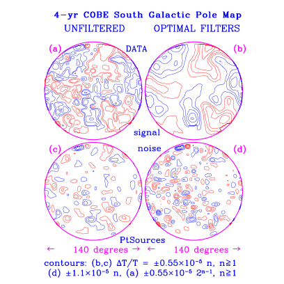
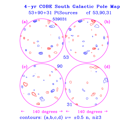
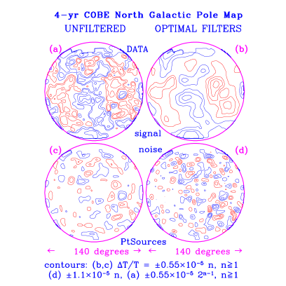
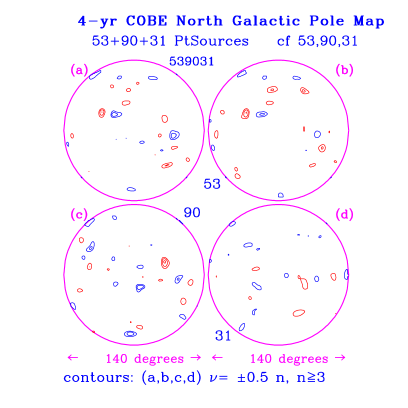
Figure 8.  : The upper left panel shows the unfiltered DMR map (combined 53+90+31 GHz data) of a $140^{\circ}$ diameter region centered on the South Galactic Pole, with the contours indicated, (b) and (d) show the Wiener-filtered signal and noise maps, while (c) shows the fluctuations of height $\nu\sigma$, with $|\nu|>1.5$. The lower left panel shows the same for the North Galactic Pole. Note the similarity between (c) and (d), that is that the Point Sources found at these low contours are consistent with random concentrations of noise, the logical conclusion within the statistics: there are no rare events that are good source candidates. We chose such a low cut so that one could see the effects of making $2$ or $3\sigma$ cuts just by counting in, each positive contour being 0.5 higher than the previous. The right panels show the contours of $\nu$ rather than $\Delta T/T$ for the individual (A+B) frequency maps. A true source would be expected to persist in the three maps, as well as being in the combined one, the strength variation across channels depending upon the emission mechanism. Again there are no obvious hits. Apart from being a useful way to detect point sources, this is a nice mechanism for looking for anomalous local non-Gaussian patterns, to be investigated to determine if we are dealing with funny noise or true signals by appropriate follow-up investigations.

3.8 Comparing: The simplest way to compare data sets A and B is to interpolate on overlap regions dataset A onto the pixels of dataset B. This of course will not always be possible, especially if the pixels are generalized ones, e.g., modal projections such as in the SK95 dataset. We would also like to compare nearby regions even if overlap is only partial. This requires an extrapolation as well as interpolation. In [55], a simple mechanism was described based upon Bayesian methods and a Gaussian interpolating theory for comparing CMB data sets. The statistics of the two experiments is defined by a joint probability for the two datasets, ${\cal P}(A,B|C_{T})$, where the theory matrix $C_{T}$ has $AB$ as well as $AA$ and $BB$ parts connecting it. A probability enhancement factor $\beta=\ln{\cal P}(A|B,C_{T})/{\cal P}(A|C_{T})$ was introduced, which is invariant under $A,B$ interchange.

What was visually instructive was to compare the A-data Wiener-filtered onto B-pixels, ${\langle s_{B}|\Delta_{A}\rangle}=C_{T,BA}\widetilde{W}_{t,AA}\overline{\Delta}_{A}$, with the Wiener-filter of B-data, ${\langle s_{B}|\Delta_{B}\rangle}=C_{T,BB}\widetilde{W}_{t,BB}\overline{\Delta}_{B}$. They should bear a striking resemblance except for the errors. The example used in [55] was SK95 data for A and MSAM92 for B, which showed remarkable similarities: indeed that the two experiments were seeing the same sky signal, albeit with some deviations near the endpoint of the scan. Although these extrapolations and interpolations are somewhat sensitive to the interpolating theory, if it is chosen to be nearly the best fit the results are robust.

The same techniques were used for an entirely different purpose in [56], testing whether two power spectra with appropriate errors, in this case from Boomerang and Maxima, could have been drawn from the same underlying distribution. The conclusion was yes.

3.9 Compressing: We would like to represent in a lossless way as much information as we can in much smaller datasets. Timestreams to maps (and map-orthogonal noise) are a form of compression, from $N_{tbits}$ to $N_{pix}$. Map manipulations, even for Gaussian theories, are made awkward because the total weight matrix involves $C_{N}$, often simplest in structure in the pixel basis, and $C_{T}$, which is often naturally represented in a spherical harmonic basis. Signal-to-noise eigenmodes $\xi_{k}$ are a basis in which $\widetilde{C}_{N}^{-1/2}C_{T}\widetilde{C}_{N}^{-1/2}$ is diagonal, hence are statistically independent of each other if they are Gaussian. They are a complete representation of the map. Another S/N basis of interest is one in which $C_{T}^{1/2}\widetilde{C}_{N}^{-1}C_{T}^{1/2}$ is diagonal, since $\widetilde{C}_{N}^{-1}$ comes out directly from the signal/noise extraction step. Finding the S/N modes is another $O(N_{pix}^{3})$ problem. Typically, ${\langle\xi_{k}^{2}\rangle}$ falls off dramatically at some $k$, and higher modes of smaller eigenvalues can be cut out without loss of information. These truncated bases can be used to test the space of theoretical models by Bayesian methods e.g., [64], and determine cosmic parameters. Further compression to bandpowers is even better for more rapid determination of cosmic parameters.

The related compression concept of parameter eigenmodes mentioned in § 1.4 finds linear combinations of the cosmological or other variables $y_{\alpha}$ that we are trying to determine which are locally statistically-independent on the multidimensional likelihood surface. It provides a nice framework for dealing with near-degeneracies.

3.10 Power Spectra and Parameter Estimation: Determining the statistical distributions of any target parameters characterizing the theories, whether they are cosmological in origin or power amplitudes in bands or correlation function in angular bins, is a major goal of CMB analysis. For power spectra and correlation functions, it is natural that these would involve pairs of pixels. Operators linear in pixel pairs are called quadratic estimators. Maximum likelihood expressions of parameters in Gaussian theories also often reduce to calculating such quadratic forms, albeit as part of iteratively-convergent sequences. Hence the study of quadratic estimators has wide applicability.

3.10.1 Quadratic Estimators: Estimating power spectra and correlation functions of the data has traditionally been done by minimizing a $\chi^{2}$ expression,

$$\chi^{2}=Tr[W(\overline{\Delta}\overline{\Delta}^{\dagger}-C(y))W(\overline{\Delta}\overline{\Delta}^{\dagger}-C(y))]\,/\,4,$$ (18)

where $W$ is some as yet unspecified weight matrix. The $1/4$ is from the pair sum. The critical element is to make a model $C(y)$ for the pixel pair correlation $\overline{\Delta}\overline{\Delta}^{\dagger}$ which is as complete a representation as possible. For example, if we adopt a linear dependence about some fiducial $C_{*}=C(y_{*})$, i.e., $C(y)=C_{*}+\sum_{\beta}C_{\beta}\delta y^{\beta}$, then

$$\sum_{\beta}{\cal F}_{\alpha\beta}\delta y^{\beta}={\textstyle{1\over 2}}{\rm Tr}[WC_{\alpha}W(\overline{\Delta}\overline{\Delta}^{\dagger}-C_{*})],\ \ C_{\alpha}\equiv\partial C/\partial y^{\alpha}\,,$$ (19)

$${\cal F}_{\alpha\beta}\equiv{\textstyle{1\over 2}}{\rm Tr}[WC_{\alpha}WC_{\beta}]-{\textstyle{1\over 2}}{\rm Tr}[WC_{\alpha\beta}W(\overline{\Delta}\overline{\Delta}^{\dagger}-C_{*})],\ \ C_{\alpha\beta}\equiv{\partial^{2}C\over\partial y^{\alpha}\partial y^{\beta}},$$

$${\rm Fisher\ information\ matrix}:\ \ F_{\alpha\beta}\equiv{\langle{\cal F}_{\alpha\beta}\rangle}={\textstyle{1\over 2}}{\rm Tr}[WC_{\alpha}WC_{\beta}]\,.$$ (20)

Since ${\cal F}_{\alpha\beta}$ has $\Delta$ dependence, this is not strictly a quadratic estimator. However, it is if the Fisher matrix $F_{\alpha\beta}$, the ensemble average of ${\cal F}_{\alpha\beta}$, is used. Iterations with $F$ rather than ${\cal F}$ converge to the same $y_{*}$ if $y$ is continually updated by the $\delta y$. $C_{*}=C_{N}+C_{T}$ has been assumed.

The correlation in the parameter errors can be estimated from the average of a quartic combination of pixel values,

$${\langle\delta y\delta y^{\dagger}\rangle}={\cal F}^{-1}{\textstyle{1\over 2}}{\rm Tr}[WC_{\alpha}WCWC_{\beta}WC]{\cal F}^{-1}$$

$$\quad\qquad+{\cal F}^{-1}{\textstyle{1\over 4}}{\rm Tr}[WC_{\alpha}W(\delta C)]{\rm Tr}[WC_{\beta}W(\delta C)]{\cal F}^{-1}\,,$$

where $(\delta C)\equiv C-C_{*}.$ Note, ${\langle\delta y\delta y^{\dagger}\rangle}={\cal F}^{-1}$ if $C=C_{*}$ and $\ W=C_{*}^{-1}.$

Another approach is to estimate the errors by taking the second derivative of $\chi^{2}$, $\partial\chi^{2}/\partial y^{\alpha}\partial y^{\beta}$ = ${\cal F}_{\alpha\beta}$:

$${\langle\partial^{2}\chi^{2}/\partial y_{\alpha}\partial y_{\beta}\rangle} ={\textstyle{1\over 2}}{\rm Tr}[WC_{\alpha}WC_{\beta}]-{\textstyle{1\over 2}}{\rm Tr}[WC_{\alpha\beta}W(\delta C)]$$

$$\rightarrow F_{\alpha\beta}\ {\rm as}\ (\delta C)\rightarrow 0.$$

These two limiting cases hold for the maximum likelihood solution as we now show.

3.10.2 Maximum Likelihood Estimators & Iterative Quadratics: The maximum likelihood solution for a Gaussian signal plus noise is of the form eq.(19) with $W=\widetilde{W}_{t}=(\widetilde{C}_{N}+C_{T}(y))^{-1}$, the “optimal” weight which gives the minimum error bars. This is found by differentiating $-2\ln{\cal L}={\rm Tr}[\widetilde{W}_{t}\overline{\Delta}\overline{\Delta}^{\dagger})]-{\rm Tr}[\ln\widetilde{W}_{t}]+N_{pix}\ln(2\pi)$. Of course the $y_{\beta}$ dependence of $\widetilde{W}_{t}$ means the expression is not really a quadratic estimator. A solution procedure is the Newton-Raphson method, with the weight matrix updated in each iterative improvement $\delta y_{\beta}$ to $y_{*\beta}$, at a cost of a matrix inversion. At each step we are doing a quadratic estimation, and when the final state has been converged upon, the weight matrix can be considered as fixed. Solving for the roots of $\partial\ln{\cal L}/\partial y_{\alpha}$ using the Newton-Raphson method requires that we calculate $\partial^{2}\ln{\cal L}/\partial y_{\alpha}\partial y_{\beta}$, the curvature of the likelihood function. Other matrices have been used for expediency, since one still converges on the maximum likelihood solution; in particular the curvature matrix expectation value, i.e., the Fisher matrix $F_{\alpha\beta}$, which is easier to calculate than ${\cal F}_{\alpha\beta}$. Further, to ensure stability of the iterative Newton-Raphson method, some care must be taken to control the step size each time the $y_{\beta}$ are updated. Since the ${\langle\delta y_{\alpha}\delta y_{\beta}\rangle}$ estimate is just $[{\cal F}^{-1}]_{\alpha\beta}$, this matrix must at least be determined after convergence to characterize the correlated errors.

Note that only in the Gaussian and uniform prior cases is the integration over $s_{(j)}$ analytically calculable, although maximum likelihood equations can be written for simple forms that can be solved iteratively, e.g., maximum entropy priors.

3.10.3 The Bandpower Case: The bandpower associated with a given window function $\varphi_{b\ell}$ of a theory with spectrum ${\cal C}_{T\ell}$ is defined as the average power,

$${\langle{\cal C}_{\ell}\rangle}_{b}\equiv{\cal I}[\varphi_{b\ell}{\cal C}_{T\ell}]/{\cal I}[\varphi_{b\ell}],$$ (21)

with ${\cal I}$ defined by eq.(7). Many choices are possible for $\varphi_{b\ell}$, but the simplest is probably the best: e.g., $\chi_{b}(\ell)$ which is unity in the $\ell$-band, zero outside. Another example uses the average window function of the experiment, $\overline{{\cal W}}_{\ell}\chi_{b}(\ell)$; others use window functions related to relative amounts of signal and noise. There is some ambiguity in the choice for the filter $\varphi_{b\ell}$  [57, 58], but often not very much sensitivity to its specific form.

We want to estimate bandpowers $q^{b}$ taken relative to a general shape ${\cal C}^{(s)}_{\ell}$ rather than the flat shape: $q^{b}\equiv{\cal I}(\varphi_{b\ell}{\cal C}_{T\ell})/{\cal I}(\varphi_{b\ell}{\cal C}^{(s)}_{\ell})$, so ${\langle{\cal C}\rangle}_{b}=\bar{q}_{b}{\langle{\cal C}^{(s)}\rangle}_{b}$. We therefore model $\overline{\Delta}\overline{\Delta}^{\dagger}$ by

$$C_{pp^{\prime}}(q)=\widetilde{C}_{N,pp^{\prime}}+\sum_{b}C^{(s)}_{b,pp^{\prime}}q^{b}\equiv C_{*,pp^{\prime}}+\sum_{b}C^{(s)}_{b,pp^{\prime}}\delta q^{b},$$

$$C^{(s)}_{b,pp^{\prime}}={\cal I}[{\cal W}_{pp^{\prime},\ell}\chi_{b}(\ell){\cal C}_{\ell}^{(s)}]\,,\qquad\delta q^{b}=q^{b}-q^{b}_{*}\,.$$ (22)

Here the $q^{b}_{*}$ are the bandpowers on a last iteration, ultimately converging to maximum likelihood bandpowers if the relaxation is allowed to go to completion, $\delta q^{b}\rightarrow 0$. The pixel-pixel correlation matrices $C_{Tb,pp^{\prime}}=C^{(s)}_{b,pp^{\prime}}q^{b}$ for the bandpowers $b$ follow from eq.(6).

The usual technique [14] is to use this linear expansion in the $q^{b}$, the downside being that the bandpowers could be negative – when there is little signal and the pixel pair estimated signal plus noise is actually less than the noise as estimated from $C_{N}$. By choosing $\exp(q^{b})$ rather than $q^{b}$ as the variables, positivity of the signal bandpowers can be assured. (The summation convention for repeated indices is often used here.)

The full maximum likelihood calculation has been used for bandpower estimates for COBE, SK95, Boomerang and Maxima, among others. The cost is ${\cal O}(N_{pix}^{3})$ for each iteration, so this limits the number of pixels that can be treated. For $N_{pix}\mathrel{\hbox to0.0pt{\lower 3.0pt\hbox{$\mathchar 536\relax$}\hss}\raise 2.0pt\hbox{$\mathchar 318\relax$}}2\times 10^{5}$ or so, the required computing power becomes prohibitive, requiring 640 Gb of memory and of order $3\times 10^{17}$ floating-point operations, which translates to a week or more even spread over a Cray T3E with $\sim 1024$ 900-MHz processors. This will clearly be impossible for the ten million pixel Planck data set. Numerical roundoff would be prohibitive anyway.

The compressed bandpowers estimated from all current data and the satellite forecasts shown in Fig. 3 were also computed using the maximum likelihood Newton-Raphson iteration method (for rather fewer “pixels”).

3.10.4 A Wavenumber-basis Example: There is an instructive case in which to unravel the terms of eq.(19). If we assume the noise and signal-shape correlation matrices in the wavenumber basis ${\bf Q}$ of § 3.4, $\widetilde{C}_{N,{\bf Q}{\bf Q^{\prime}}}$ and $C^{(s)}_{Tb,{\bf Q}{\bf Q^{\prime}}}$, are functions only of the magnitude of the wavenumber, $Q\approx\ell+{\textstyle{1\over 2}}$, then

$$\sum_{b^{\prime}}F_{bb^{\prime}}q^{b^{\prime}}={\textstyle{1\over 2}}\sum_{Q}g_{Q}W^{2}(Q)C_{Tb}^{(s)}(Q)(C_{est}(Q)-\widetilde{C}_{N}(Q))\,,$$ (23)

$$F_{bb^{\prime}}={\textstyle{1\over 2}}\sum_{Q}g_{Q}W^{2}(Q)C^{(s)}_{Tb}(Q)C^{(s)}_{Tb^{\prime}}(Q)\,,$$

$$W(Q)=(\widetilde{C}_{N}(Q)+\sum_{b}C^{(s)}_{Tb}(Q)q_{*}^{b})^{-1}\,\quad C_{est}(Q)\equiv\int{d\phi_{\bf Q}\over 2\pi}\,|\overline{\Delta}_{\bf Q}|^{2}\,.$$

Here $g_{Q}$ is the effective number of modes contributing to the $\Delta Q$=1 wavenumber interval.

In the all-sky homogeneous noise limit, this of course gives the correct result, with $g_{Q}=f_{sky}(2\ell+1)$ and $C^{(s)}_{Tb}(Q)=C^{(s)}_{\ell}\overline{{\cal W}}_{\ell}\chi_{b}(\ell)$, where $\overline{{\cal W}}_{\ell}$ is the window (the angle-average of $|u({\bf Q})|^{2}{\cal B}_{\ell}^{2}$ in the language of § 3.4.1). Since $\chi_{b}(\ell)\chi_{b^{\prime}}(\ell)=\delta_{bb^{\prime}}(\ell)\chi_{b}(\ell)$, $F_{bb^{\prime}}$ is diagonal, with a value expressed in terms of a band-window $\varphi_{b\ell}$:

$$F_{bb}={\textstyle{1\over 2}}{\cal I}[\varphi_{b\ell}{\cal C}^{(s)}_{\ell}],\quad\varphi_{b\ell}=4\pi(g_{Q}/(2Q))W^{2}(Q)C_{\ell}^{(s)}\overline{{\cal W}}_{\ell}^{2}\chi_{b}(\ell)\,.$$ (24)

It may now seem that we have identified up to a normalization the correct band-window to use in this idealized case, with a combination of signal and noise weighting. However the ambiguity referred to earlier remains, for what we are actually doing in estimating the observed $q^{b}$ is building a piecewise discontinuous model relative to the shape ${\cal C}^{(s)}_{\ell}$. The analogue for a given ${\cal C}_{T\ell}$ is the model $\sum_{\ell}\chi_{b}(\ell)q_{Tb}{\cal C}^{(s)}_{\ell}$. Since for the theory, $q^{b}={\cal I}[\varphi_{b\ell}{\cal C}_{T\ell}]/{\cal I}[\varphi_{b\ell}{\cal C}^{(s)}_{\ell}]$, any $\varphi_{b\ell}$ satisfying $\varphi_{b\ell}\chi_{b^{\prime}}(\ell)$ = $\varphi_{b\ell}$ will do to have $q_{Tb}$ the ratio of target-bandpower to shape-bandpower.

The downweighting by signal-plus-noise power is just what is required to give the correct variance in the signal power estimate in the limit of small bin size:

$${\langle(\Delta{\cal C}_{Tb})^{2}\rangle}=F_{bb}^{-1}{\langle{\cal C}_{\ell}^{(s)}\rangle}_{b}^{2}\rightarrow{2\over g_{\ell}}{({\cal C}_{T\ell}\overline{{\cal W}}_{\ell}+\widetilde{{\cal C}}_{N\ell})^{2}\over\overline{{\cal W}}_{\ell}^{2}}\ {\rm as}\ \Delta\ell\rightarrow 1\,.$$ (25)

In the sample-variance dominated regime, the error is ${\cal C}_{T\ell}\sqrt{2/g_{\ell}}$, while in the noise-dominated regime it is $\widetilde{{\cal C}}_{N\ell}\sqrt{2/g_{\ell}}/\overline{{\cal W}}_{\ell}$, picking up enormously above the Gaussian beam scale. Recent experiments are designed to have signal-to-noise near unity on the beam scale, hence are sample-variance dominated for lower $\ell$. The interpretation of the $(\widetilde{C}_{N\ell}+C_{T\ell})^{-1}$ weighting factor is that correlated spatial patterns associated with a wavenumber $\ell$ that are statistically high just because of sample variance are to be downweighted by $C_{T\ell}$.

Although these results are only rigorous for the all-sky case with homogeneous and isotropic noise, they have been used to great effect for forecasting errors (§3.11) for $f_{sky}<1$ regions.

3.10.5 Faster Bandpowers: Since the need for speed to make the larger datasets tractable is essential, much attention is now being paid to much faster methods for bandpower estimation.

A case has been made for highly simplified weights (e.g., diagonal in pixel space) that would still deliver the basic results, with only slightly increased error bars [60]. The use of non-optimal weighting schemes has had a long history. For example, a quadratic estimator of the correlation function was used in the very first COBE DMR detection publication, with $diag(W_{N})$ for $W$, a choice we have also used for COBE and the balloon-borne FIRS. Here one is estimating correlation function amplitudes $C^{\alpha}$, where $\alpha$ refers to an angular bin: $C_{pp^{\prime}}=C_{Npp^{\prime}}+\sum_{\alpha}C^{\alpha}\chi_{\alpha}(\theta_{pp^{\prime}})$, where $\cos(\theta_{pp^{\prime}})={\hat{q}}_{p}\cdot{\hat{q}}_{p^{\prime}}$ and $\chi_{\alpha}(\theta)$ is one inside and zero outside of the bin. As for bandpowers, the distribution is non-Gaussian, so errors were estimated using Monte Carlo simulations of the maps.

Any weight matrix $W$ which is diagonal in pixel space is easy and fast to calculate. In [60] it was shown that making $W$ the identity was adequate for Boomerang-like data. The actual approach used a fast highly binned estimate of $C(\theta)$, which can be computed quickly, which was then lightly smoothed, and finally a Gauss-Legendre integration of $C(\theta)$ was done to estimate ${\langle{\cal C}\rangle}_{b}$.

One can still work with the full $W=\widetilde{W}_{t}$ if the noise weight matrix $C_{N}^{-1}$ has a simple form in the pixel basis. For the MAP satellite, it is nearly diagonal, and a method exploiting this has been applied to MAP simulations to good effect [61].

Since many of the signals are most simply described in multipole space, it is natural to try to exploit this basis, especially in the sample-variance dominated limit. In the Boomerang analysis of [4, 38], filtering of form $\mu(\varpi_{p})u({\bf Q}){\cal B}(Q)$ was imposed. Many of the features of the diagonal ansatz of § 3.10.4 in wavenumber space were exploited, complicated of course by the spatial mask $\mu$, which leads to mode-mode coupling. The main approximation was to use the masked transforms for the basic isotropic $Q$ functions, expressing where needed the masked power spectra as linear transformations on the true underlying power spectrum in $\ell$-space that we are trying to find. Monte Carlo simulations were used to evaluate a number of the terms. Details are given in [4, 38] and elsewhere.

More could be said about making power spectrum estimation nearly optimal and also tractable, and much remains to be explored.

3.10.6 Relating Bandpowers to Cosmic Parameters: To make use of the $q^{b}$ for cosmological parameter estimation, we need to know the entire likelihood function for $q^{b}$, and not just assume a Gaussian form using the curvature matrix. This can only be done by full calculation, though there are two analytic approximations that have have been shown to fit the one-point distributions quite well in all the cases tried [57]. The simplest and most often used is an “offset lognormal” distribution, a Gaussian in $z^{b}=\ln(q^{b}+q_{N}^{b})$, where the offset $q_{N}^{b}$ is related to the noise in the experiment:

$${\cal P}(q)\propto\exp[-{\textstyle{1\over 2}}(z-\bar{z})^{b}{\cal F}^{(z)}_{bb^{\prime}}(z-\bar{z})^{b^{\prime}}],$$

$${\cal F}^{(z)}_{bb^{\prime}}=(\bar{q}^{b}+q_{N}^{b}){\cal F}^{(q)}_{bb^{\prime}}(\bar{q}^{b^{\prime}}+q_{N}^{b^{\prime}}),$$

$$\bar{q}^{b}/q_{N}^{b}=[{\cal F}^{(q)0}_{bb^{\prime}}/{\cal F}^{(q)}_{bb^{\prime}}]^{1/2}-1\,,$$ (26)

where $\bar{q}^{b}$ is the maximum likelihood value. To evaluate $q_{N}^{b}$ in eq.(26), the curvature matrix evaluated in the absence of signal, ${\cal F}^{(q)0}_{bb^{\prime}}$, is needed. For Boomerang and Maxima analysis, the two Fisher matrices are standard output of the “MADCAP” maximum likelihood power spectrum estimation code [59]. Another (better) approach if the likelihood functions ${\cal L}(\{q^{b}\})$ are available for each $q^{b}$ is to fit $\ln{\cal L}$ by $-{\textstyle{1\over 2}}[(z-\bar{z})_{b}]^{2}g_{b}^{2}$, and use $g_{b}G_{bb^{\prime}}g_{b^{\prime}}$ in place of ${\cal F}_{bb^{\prime}}^{(z)}$, where $G_{bb^{\prime}}=diag({\cal F}^{-1})^{1/2}{\cal F}diag({\cal F}^{-1})^{1/2}$. Here $diag()$ denotes the diagonal part of the matrix in question. Values of $q_{N}^{b}$ and other data for a variety of experiments are given in [57] (where it is called $x^{b}$). It is also possible to estimate $q_{N}^{b}$ using a quadratic estimator [4]. To compare a given theory with spectrum ${\cal C}_{T\ell}$ with the data using eq.(26), the $q^{b}$’s need to be evaluated with a specific choice for $\varphi_{b\ell}$. Although this should be band-limited, $\propto\chi_{b\ell}$, as described in § 3.10.4, the case can be made for a number of alternate forms.

3.11 Forecasting: A typical forecast involves making large simplifications to the full statistical problem, such as those used in § 3.10.4. For example, the noise is homogeneous, possibly white, and the fluctuations are Gaussian. This was applied to estimates of how well cosmic parameters could be determined for the LDBs and MAP and Planck in the 9 parameter case described earlier [13], and for cases where the power spectrum parameters are allowed to open up beyond just tilts and amplitudes to parameterized shapes [62]. The methods were also applied when CMB polarization was included, and when LSS and supernovae were included [63].

The procedure is exactly like that for maximum likelihood parameter estimation, except one often does not bother with a realization of the power spectrum, rather uses the average (input) value and estimates errors from the ensemble average curvature, i.e., the Fisher matrix: $F^{-1}$ is therefore a measure of ${\langle\delta y_{\alpha}\delta y_{\beta}\rangle}$, where $\delta y_{\alpha}=y_{\alpha}-\bar{y}_{\alpha}$ is the fluctuation of $y_{\alpha}$ about its most probable value, $\bar{y}_{\alpha}$. As mentioned above, when the $y_{\alpha}$ are the bandpowers instead of the cosmic parameters, we get the forecasts of power spectra and their errors, as for MAP and Planck in Fig. 3. Those results ignored foregrounds. However other authors have treated foregrounds with the Gaussian and max-ent prior assumptions in this simplified noise case [45, 47].

Clearly forecasting can become more and more sophisticated as realistic noise and other signals are added, ultimately to grow into a full pipeline-testing simulation of the experiment, which all of the CMB teams strive to do to validate their operations.

Challenge: The lesson of the CMB analysis done to date is that almost all of the time and debate is spent on the path to a believable primary power spectrum, with the cosmological parameters quickly dropping out once the spectrum has been agreed upon. The analysis challenge, requiring clever new algorithms, gets more difficult as we move to more LDBs and interferometers, to MAP and to Planck. This is especially so with the ramping-up efforts on primary polarization signals, expected at $<$10% of the total anisotropies, and the growing necessity to fully confront secondary anisotropies and foregrounds simultaneously with the primary signals.

Acknowledgments: Many people have worked with us at CITA on aspects of the CMB analysis touched on here, Carlo Contaldi, Andrew Jaffe, Lloyd Knox, Steve Myers, Barth Netterfield, Ue-Li Pen, Dmitry Pogosyan, Simon Prunet, Marcelo Ruetalo, Kris Sigurdson, Tarun Souradeep, Istvan Szapudi, and James Wadsley, along with Julian Borrill, Eric Hivon and other members of the Boomerang and CBI teams, and George Efstathiou and Neil Turok at Cambridge.

References

- [1] Seljak, U. and Zaldarriaga, M. 1996, ApJ 469, 437. (CMBfast)
- [2] Miller, A.D. et al. 1999, ApJ 524, L1. (TOCO)
- [3] de Bernardis, P. et al. 2000, Nature 404, 995.
- [4] Netterfield, C.B. et al. 2001, astro-ph/0104460; de Bernardis, P. et al. 2001, astro-ph/0105296. (BOOM)
- [5] Mauskopf, P. et al. 2000, ApJ Lett 536, L59. (BOOM-NA)
- [6] Hanany, S. et al. 2000, ApJ Lett. 545, 5.
- [7] Lee, A.T. et al. 2001, astro-ph/0104459; Stompor, R. et al. 2001, astro-ph/0104462. (MAXIMA)
- [8] Padin, S. et al. 2000, ApJ Lett., submitted, astro-ph/0012211; Myers, S. et al. 2001, preprint. (CBI)
- [9] Leitch, E.M. et al. 2001, astro-ph/0104488; Halverson, N.W. et al. 2001, astro-ph/0104489; Pryke, C. et al. 2001, astro-ph/0104490. (DASI)
- [10] Bond, J.R. 1996, in Cosmology and Large Scale Structure, Les Houches Session LX, eds. R. Schaeffer J. Silk, M. Spiro and J. Zinn-Justin (Elsevier), pp. 469-674
- [11] Bond, J.R. 1994, Phys. Rev. Lett. 74, 4369.
- [12] e.g., Efstathiou, G. & Bond, J.R. 1999, M.N.R.A.S. 304, 75, where many other near-degeneracies between cosmological parameters are also discussed.
- [13] Bond, J.R., Efstathiou, G. & Tegmark, M. 1997, M.N.R.A.S. 291, L33.
- [14] Bond, J.R., Jaffe, A.H. & Knox, L. 1998, Phys. Rev. D 57, 2117.
- [15] Pen Ue-Li, Seljak U. & Turok N. 1997, Phys. Rev. Lett. 79, 1611.
- [16] Allen, B., Caldwell, R.R., Dodelson, S., Knox, L., Shellard, E.P.S. & Stebbins, A. 1997, astro-ph/9704160.
- [17] Frenk, C.S. et al. 1999, ApJ 525, 554.
- [18] Birkinshaw, M. 1999, Phys. Rep. 310, 97.
- [19] Wadsley, J.W. & Bond, J.R. 2001, preprint.
- [20] Bond, J.R., Pogosyan, D., Kofman, L. & Wadsley, J.W. 1998, in “Wide Field Surveys in Cosmology”, Proc. XIV IAP Colloquium Conf., ed. S. Colombi & Y. Mellier, (Paris: Editions Frontieres), p. 17, astro-ph/9810093.
- [21] Pogosyan, D., Bond, J.R., Kofman, L. & Wadsley, J.W. 1998, in “Wide Field Surveys in Cosmology”, Proc. XIV IAP Colloquium Conf., ed. S. Colombi & Y. Mellier, (Paris: Editions Frontieres), p. 61, astro-ph/9810072.
- [22] Persi, F.M., Spergel, D.N., Cen, R. & Ostriker, J.P. 1995, ApJ 442, 1.
- [23] Refregier, A., Komatsu, E., Spergel, D.N. & Pen, Ue-Li 2000, astro-ph/9912180.
- [24] Scaramella, R., Cen, R. & Ostriker, J.P. 1993, ApJ 416, 399.
- [25] Seljak, U., Burwell, J. & Pen, Ue-Li 2000, astro-ph/0001120.
- [26] da Silva, A.C., Barbosa, D., Liddle, A.R. & Thomas, P.A. 2000, MNRAS 317, 37.
- [27] Springel, V., White, M. & Hernquist, L. 2000, astro-ph/0008133.
- [28] Bond, J.R. 1988, in The Early Universe, Proc. NATO Summer School, Victoria, B.C., Canada, August 1986, p. 283-334, ed. W. Unruh and G. Semenoff, Dordrecht: Reidel.
- [29] Bond, J.R., Carr, B.J. & Hogan, C.J. ApJ 1991, 367, 420.
- [30] Bond, J.R. & Myers, S. 1996, ApJ Supp 103, 1, 41; 63.
- [31] Bond, J.R., Ruetalo, M. & Wadsley, J.W. 2001, in Proc. TAW8 conference on High Redshift CLusters, Missing Baryons and CMB Polarization.
- [32] Lange, A. et al. 2001, Phys. Rev D, in press.
- [33] Bond, J.R., Crittenden, R., Jaffe, A.H. & Knox, L. 1999, Computing in Science and Engineering 1, 21, astro-ph/9903166, and references therein.
- [34] Ferreira, P.G. & Jaffe, A.H. 1999, M.N.R.A.S. astro-ph/9909250.
- [35] Prunet, S. et al. 2001, Proc. Garching Conference on “Analysis of Large Astronomical Data Sets”, astro-ph/0101073.
- [36] Stompor, R. et al. 2001, Proc. Garching Conference on “Analysis of Large Astronomical Data Sets”, astro-ph/0012418.
- [37] Dore, O., Teyssier, R., Bouchet, F.R., Vibert, D. & Prunet, S. 2001, AstronAp, astro-ph/0101112.
- [38] Hivon, E., Gorksi, K.M., Netterfield, C.B., Crill, B.P., Prunet, S., Hansen, F. 2001, ApJ, astro-ph/0105302.
- [39] Stompor, R. et al. 2001, Phys. Rev. D, astro-ph/0106451.
- [40] Hinshaw, G. et al. 2001, Proc. Garching Conference on “Analysis of Large Astronomical Data Sets”, astro-ph/0011555; see also E.L. Wright 1996, astro-ph/9612006.
- [41] Muciaccia, P.F., Natoli, P. & Vittorio, N. 1998, ApJ 488, L63.
- [42] Gorski, K.M., Hivon, E. & Wandelt, B.D. 1998, astro-ph/9812350.
- [43] Crittenden, R. & Turok, N. 1999, astro-ph/9806374.
- [44] Hobson, M.P. & Lasenby, A.N. 1998, M.N.R.A.S. 298, 905.
- [45] Bouchet, F.R. & Gispert, R. 1999, New Astron. 4, 443.
- [46] Prunet, S. et al. 2000b, AstronAp Lett, astro-ph/0012497.
- [47] Hobson, M.P., Jones, A.W., Lasenby, A.N. & Bouchet, F.R. 1999, M.N.R.A.S. astro-ph/9806387.
- [48] Schlegel, D.J., Finkbeiner, D.P. & Davis, M. 1998, ApJ 500, 525.
- [49] Jaffe, A.H., Finkbeiner, D. & Bond, J.R. 1999, preprint.
- [50] de Oliveira-Costa, A., et al. 1997, ApJ Lett 482, 17.
- [51] Crittenden, R. & Bond, J.R. 2001, preprint.
- [52] Tegmark, M. and de Oliveira-Costa, A. 1998, ApJ 500, 83.
- [53] Haehnelt, M.G. & Tegmark. M. 1996, M.N.R.A.S. 279, 545.
- [54] Cayon, L. et al. 2000, M.N.R.A.S. astro-ph/9912471
- [55] Knox, L., Bond, J.R., Jaffe, A.H., Segal, M. & Charbonneau, D. 1998, Phys. Rev. D, 58, 1443.
- [56] Jaffe, A.H. et al. 2001, Phys. Rev. Lett., in press.
- [57] Bond, J.R., Jaffe, A.H. & Knox, L. 2000, ApJ 533, 19.
- [58] Knox, L. 2000, Phys. Rev. D, astro-ph/9902046.
- [59] Borrill, J. 1999, Phys. Rev. D 59, 7302.
- [60] Szapudi, I., Prunet, S., Pogosyan, D., Szalay, A. & Bond, J.R. 2001, ApJ Lett, in press.
- [61] Oh, S.P., Spergel, D.N. & Hinshaw, G. 1999, ApJ 510, 551.
- [62] Souradeep, T., Bond, J.R., Knox, L., Efstathiou, G. & Turner, M.S. 1998, in “Proceedings of COSMO-97”, ed. L. Roszkowski (World Scientific), astro-ph/9802262.
- [63] Eisenstein, D., Hu, W. & Tegmark, M. 1998, ApJ, astro-ph/9807130.
- [64] Bond, J.R. & Jaffe, A. 1998, Phil. Trans. R. Soc. London 357, 57.
- [65] Bond, J.R. et al. 2000, Proc. IAU Symposium 201, astro-ph/0011378; Proc. CAPP 2000, astro-ph/0011379; Proc. Neutrino 2000, astro-ph/0011377.
- [66] Bond, J.R., Pogosyan, D. and Souradeep, T. 2000, Phys. Rev. D 62.