IFIC/01-38

HD-THEP-01-30

Imperial/TP/0-01/23

DAMTP-2001-66

astro-ph/0108093

August 2001

NATURAL MAGNETOGENESIS FROM INFLATION

K. Dimopoulos,¹ T. Prokopec,² O. Törnkvist³ and A. C. Davis⁴

¹Instituto de Física Corpuscular, Universitat de Valencia/CSIC,
Apartado de Correos 22085, 46071 Valencia, Spain

²Institute for Theoretical Physics, Heidelberg University,
Philosophenweg 16, D-69120 Heidelberg, Germany

³Theoretical Physics Group, Imperial College
Prince Consort Road, London SW7 2BZ, U.K.

⁴Department of Applied Mathematics and Theoretical Physics, University of Cambridge,
Wilberforce Road, Cambridge CB3 0WA, United Kingdom

Abstract

We consider the gravitational generation of the massive $Z$ boson field of the standard model, due to the natural breaking of its conformal invariance during inflation. The electroweak symmetry restoration at the end of inflation turns the almost scale-invariant superhorizon $Z$ spectrum into a hypermagnetic field, which transforms into a regular magnetic field at the electroweak phase transition. The mechanism is generic and is shown to generate a superhorizon spectrum of the form $B\propto 1/\ell$ on a length-scale $\ell$ regardless of the choice of inflationary model. Scaled to the epoch of galaxy formation such a field suffices to trigger the galactic dynamo and explain the observed galactic magnetic fields in the case of a spatially flat, dark energy dominated Universe with GUT-scale inflation. The possibility of further amplification of the generated field by preheating is also investigated. To this end we study a model of Supersymmetric Hybrid Inflation with a Flipped SU(5) grand unified symmetry group.

 
¹kostas@flamenco.ific.uv.es, ²T.Prokopec@ThPhys.Uni-Heidelberg.DE
³o.tornkvist@ic.ac.uk, ⁴acd@damtp.cam.ac.uk

1 Introduction

Magnetic fields permeate most astrophysical systems [1] and their presence may have numerous cosmological and astrophysical implications. Indeed, magnetic fields may substantially influence the formation process of large-scale structure [2] and of individual galaxies [3][4]. However, the most important role of large-scale magnetic fields is that they may be responsible for the magnetic fields in galaxies.

It is a well-known observational fact that galaxies feature magnetic fields of strength $\sim\mu$Gauss [1][5][6]. The structure of such fields in spiral galaxies follows closely the spiral pattern [5] and this strongly suggests that the galactic magnetic fields are generated and sustained by a dynamo mechanism [1][5][7]. According to the galactic dynamo, the cyclonic turbulent motion of ionized gas combined with the differential galactic rotation amplifies a weak seed field exponentially until the backreaction of the plasma motion counteracts the growth of the field and stabilizes it to dynamical equipartition strength. However, the origin of the required seed field remains elusive.

In order to trigger successfully the galactic dynamo, the seed field has to satisfy certain requirements of strength and coherence. Indeed, it has been shown that seed fields which are too incoherent may destabilize and destroy the dynamo action [8]. Most dynamos require a minimum coherence length comparable to the dimensions of the largest turbulent eddy, $\sim$ 100 pc. The required strength is determined by the dynamo’s amplification timescale (typically the galactic rotation period) and the age of the galaxy. Recent observations suggest that the Universe at present is dominated by a dark-energy component [9]. In such a case the galaxies are older than previously thought, and the minimum seed-field strength may be as low as $B_{\rm seed}\sim 10^{-30}$Gauss [10].

There have been attempts to generate the necessary seed field using various astrophysical mechanisms, the most important of which involve battery [11] or vorticity effects [4][12]. Battery mechanisms require a large-scale misalignment of density and pressure (temperature) gradients, usually associated with large lobe-jets (AGNs) or starburst activity [13], and are therefore difficult to realize in the majority of the galaxies. On the other hand, large-scale vortical motions can be effective only if the ionization of the plasma is substantial, which can hardly occur as late as the epoch of galaxy formation.

Due to the above difficulties, it has been frequently argued that the origin of the seed field may precede the galaxies themselves, i.e. be truly primordial. The obvious requirement for large-scale magnetic-field generation before the time of recombination is that it has to occur out of thermal equilibrium, because such a field breaks isotropy [14]. This limits the choice to generating the magnetic field either at a phase transition or during inflation, although more exotic mechanisms have occasionally been suggested, such as vorticity-inducing cosmic strings [15] or magnetic fields in the pre-Big Bang era [16].

There have been numerous attempts to create a primordial magnetic field at the breaking of grand unification or at the electroweak phase transition or even at the quark-confinement epoch (QCD transition) [17]. However, since the generating mechanisms are causal, the coherence of the created magnetic field cannot be larger than the particle horizon at the time of the phase transition. Because all the above transitions occurred very early in the Universe’s history, the comoving size of the horizon is rather small (the best case is the QCD transition, for which the horizon corresponds to $\sim$ 1 AU) and so the resulting magnetic fields are too incoherent. It has been shown that not even the most favorable turbulent evolution can adequately increase the correlation length of such fields [18]. Thus, one should achieve superhorizon correlations in order to generate a sufficiently coherent magnetic field in the early Universe.

Inflation presents the only known way to achieve correlations beyond the horizon scale and, for this reason, has received a lot of attention. However, the prime obstacle to generating magnetic fields during inflation is the conformal invariance of electromagnetism, which forces the magnetic flux to be conserved [19]. As a result, the strength of any generated magnetic field decreases exponentially as the inflationary Universe rapidly expands. Attempts to overcome this problem have set out to break the conformal invariance in various ways, such as through the explicit introduction of terms in the Lagrangian which couple the photon directly to gravity or to a scalar or pseudoscalar field, or through the inclusion of a massive photon, or even by means of the conformal anomaly [19][20]. However, those very few attempts that succeed in producing a sufficiently strong magnetic field do so relinquishing simplicity. Recently, interesting efforts have been made to create magnetic fields by coupling the photon to some scalar field during inflation [21] or at the preheating stage [22]. These proposals have since been criticized in [23]. Other recent ideas include magnetogenesis due to the breakdown of Lorentz invariance in the context of string theory and non-commutative VSL theories [24], due to the dynamics of large extra dimensions [25] and, finally, due to gauge field coupling to metric perturbations [26]. The viability of the latter has been questioned in [27].

Recently one of us (TP) has studied the effects of conformal symmetry breaking due to the coupling of the photon field to fermions and scalars [27]. The author has considered effective actions arising from loop corrections in the $1/M$ expansion and from the anomaly. In addition, the photon coupling to scalar and pseudoscalar fields was reconsidered, having been originally introduced by Ratra in [20] and in [19] (see also Garretson et al. in [20] and [28]).

In this paper we show that conformal invariance is naturally broken in inflation without the need for any exotic mechanism or field. In particular, we consider the gravitational generation of the massive $Z$-boson field of the standard model. The electroweak symmetry restoration at the end of inflation turns the superhorizon $Z$ spectrum into a hypermagnetic field, which transforms into a regular magnetic field at the electroweak phase transition. The mechanism is rather generic and is shown to generate a superhorizon spectrum of the form $B_{\rm rms}\propto 1/\ell$ on a length-scale $\ell$ regardless of the choice of inflationary model. However, it is possible to consider further amplification of the generated field via parametric resonance during preheating. To this end, we study a model of Supersymmetric Hybrid Inflation (SUSY-HI) with Flipped SU(5) as the symmetry group of the Grand Unified Theory (GUT). Our mechanism for creating the field has been described in [29], where it was not specifically applied to the $Z$ field.

The structure of our paper is as follows. In Section 2, the model of Supersymmetric Hybrid Inflation is presented. Section 3 contains a study of the relevant particle representations of the Flipped SU(5) group. The symmetry breaking process is analyzed and the field equations of the gauge bosons are obtained, with particular emphasis on the hypercharge field and its source current. Also, the equations for the scalar fields (Higgs fields and the inflaton) are layed out in detail. In Section 4, we study the gravitational production of the $Z$-boson field during inflation in a model-independent way. The resulting spectrum of the magnetic field is computed and scaled down to the epoch of galaxy formation, thus showing that it may be sufficient for explaining the galactic magnetic fields. In Section 5, the possibility of extra amplification by preheating is investigated using the particular model of Flipped-SU(5) SUSY-HI. Both Flipped SU(5) and SUSY-HI are well motivated by Supergravity and Superstrings and rather are naturally compatible. However, it should be noted that the choice of GUT group was made only to allow us to perform analytical calculations. In principle, any GUT group would suffice. Finally, in Section 6 we present our conclusions. We have attached two Appendices, one describing the Hartree approximation used at certain points in the calculations and the other presenting the way to calculate the rms amplitudes of the $Z$-boson and the hypermagnetic field.

Throughout the paper we use a $(+,-,-,-)$ metric and units with $c=\hbar=1$ so that Newton’s gravitational constant is $8\pi G=m_{P}^{-2}$, where $m_{P}=2.4\times 10^{18}$GeV is the reduced Planck mass.

2 Supersymmetric Hybrid Inflation

2.1 Hybrid Inflation

Hybrid Inflation was originally suggested by Linde [30] to avoid the fine-tuning problems of most inflationary models due to radiative corrections. In order to achieve this, Hybrid Inflation introduces a mass scale $M$, much smaller than the Planck mass, that sets the scale of the false-vacuum energy towards the end of inflation. Thus, at least near the end, the inflationary potential is protected from radiative corrections and is sufficiently flat. The expense paid is the necessity of introducing, in addition to the inflaton field $s$, another scalar field $\phi$ related to the scale $M$. The scalar potential for Hybrid Inflation is,

$$V(\phi,s)=\frac{1}{4}\lambda\left(\phi^{2}-M^{2}\right)^{2}+\frac{1}{2}hs^{2}\phi^{2}+V_{s}(s)$$ (1)

where $\lambda$ and $h$ are coupling constants and $V_{s}(s)$ is the slow-roll potential for the inflaton field. Because of the coupling between $s$ and $\phi$, for $s\geq s_{c}$, where $s_{c}\equiv M\sqrt{{\lambda}/{h}}$, the above potential has a global minimum at $\phi=0$, so that $V(0,s)=\lambda M^{4}/4$ and we obtain low energy-scale inflation as required. However, when $s<s_{c}$, spontaneous symmetry breaking displaces the minimum of the potential (1) to $\phi=M_{e\!f\!f}$, where $M_{e\!f\!f}^{2}\equiv M^{2}[1-(s/s_{c})^{2}]$. The system rapidly rolls towards the new minimum and oscillates around it, thus terminating inflation. In general, inflation ends abruptly less than one $e$-folding after the symmetry breaking.

Letting $M$ be of the order of the grand-unification scale can indeed satisfy the requirements of successful inflation, for which the total number of $e$-foldings must be large enough (typically about 60) to solve the flatness and horizon problems and to account for the magnitude of density perturbations and the anisotropy of the Cosmic Microwave Background Radiation (CMBR) in agreement with Large-Scale Structure and COBE observations. Thus, a natural candidate for the $\phi$ scalar is the Higgs field of a Grand Unified Theory (GUT). Such a choice has the merit of not introducing any additional unknown scalars or mass scales.

However, the most important attribute of Hybrid Inflation is that it can originate from Supersymmetry and is, therefore, one of the few inflationary models with a theoretical foundation in particle physics.

2.2 Supersymmetric model

The literature on Supersymmetric Hybrid Inflation (SUSY-HI) is rather rich, as it is possible to attain from either Supergravity or Superstrings [31]. We shall briefly describe an $F$-term GUT inflationary model as in [32]. $D$-term models also exist [33], but will not concern us here.

The most general renormalizable superpotential with $R$-symmetry is [32],

$$W=\kappa S(\Phi\bar{\Phi}-M^{2})$$ (2)

where $\Phi\bar{\Phi}$ is a conjugate pair of singlet components of chiral superfields that belong to a nontrivial representation of the GUT group $G$, $S$ is a gauge-singlet superfield, and $\kappa$, $M$ are constants that can be made positive by phase redefinitions. Introducing the above expression to the $F$-term scalar potential $V_{F}\simeq\sum_{i}|{\partial W}/{\partial\phi_{i}}|^{2}$ one finds,

$$V=\kappa^{2}|M^{2}-\Phi\bar{\Phi}|^{2}+\kappa^{2}|S|^{2}(|\Phi|^{2}+|\bar{\Phi}|^{2})$$ (3)

where we write the scalar components with the same symbols as the superfields. Using $R$-symmetry we can bring the scalar fields onto the real axis. We set $S\equiv s/\sqrt{2}$ and $\Phi=\bar{\Phi}\equiv\phi$, where $s$ and $\phi$ are real scalar fields. Then the scalar potential becomes,

$$V(\phi,s)=\kappa^{2}(\phi^{2}-M^{2})^{2}+\kappa^{2}s^{2}\phi^{2}$$ (4)

This is, in fact, the potential for Hybrid Inflation given in (1) with $\lambda\!=\!2h\!=4\kappa^{2}$ and $s_{c}\equiv\sqrt{2}M$.

The non-vanishing vacuum energy breaks supersymmetry and generates radiative corrections, which induce the required slow-roll potential $V_{s}(s)$. It can be shown that the overall contribution is of the form [32],

$$V_{s}(s)\simeq M^{4}\frac{\kappa^{4}}{16\pi^{2}}(\ln\frac{\sqrt{\kappa}\,s}{\Lambda}+\frac{3}{2})$$ (5)

where $\Lambda$ is a suitable renormalization mass scale. Thus, the radiative corrections provide a gentle down-slope for the inflaton, $V_{s}\propto\ln s$, which helps to drive it towards its minimum.

At earlier stages of the inflaton’s evolution, $s$ may be of the order of the Planck mass, so that Supergravity corrections should also be considered. However, it can be shown [34] that the flatness of the potential is preserved for minimal Kähler potential ($K=2\phi^{2}+S^{2}$).

3 Flipped SU(5)

In choosing the GUT for the symmetry breaking that terminates Hybrid Inflation, one has to ascertain that there is no monopole problem [35]. Thus, a simple or semi-simple group is not an option. We decided in favor of Flipped SU(5) because of its simplicity and its resemblance to the Standard Model (SM). Flipped SU(5) is jargon for the GUT group SU(5)$\times\overline{\mbox{U}}$(1), in which the hypercharge U(1)_Y is contained both in the SU(5) part and the $\overline{\mbox{U}}$(1), in contrast to the Georgi-Glashow SU(5)$\times$U(1) model, which has the hypercharge fully embedded in SU(5) [36].

The supersymmetric version of Flipped SU(5) is well motivated by Superstrings [37]. Moreover, it can be considered as an intermediate stage in the breaking of supersymmetric SO(10) [36][38]:

SO(10) $$\rightarrow\;\;\;\mbox{SU(5)$\times\overline{\mbox{U}}$(1)}\;\;\;\rightarrow {}_{c}\times \times$$ SU(3)SU(2)U(1)_Y

Since the breaking of SO(10) to Flipped SU(5) generates monopoles, it would have to take place before or during the inflationary period, so that the monopoles can be safely inflated away. The SUSY-HI in this model has been studied in [39].

3.1 The model

The Lagrangian density of the model is [40],

$${\cal L}=-\frac{1}{4}g^{\mu\rho}g^{\nu\sigma}\mbox{Tr}(G_{\mu\nu}G_{\rho\sigma})-\frac{1}{4}g^{\mu\rho}g^{\nu\sigma}G^{0}_{\mu\nu}G^{0}_{\rho\sigma}+\frac{1}{2}g^{\mu\nu}\mbox{Tr}[(D_{\mu}\Phi)^{\dagger}D_{\nu}\Phi]+\frac{1}{2}g^{\mu\nu}(\nabla_{\mu}s)\nabla_{\nu}s-V\,$$ (6)

where $\Phi$ is the GUT-Higgs field, $s$ is the inflaton field, $G_{\mu\nu}$ and $G^{0}_{\mu\nu}$ are the field strengths of the SU(5) and the $\overline{\mbox{U}}$(1) gauge fields respectively, $D_{\mu}\Phi$ is the covariant derivative of the Higgs field, and $V$ is the effective potential.

The SU(5) field strength is,

$$G_{\mu\nu}=\nabla_{\mu}\mbox{$\mit\Lambda$}_{\nu}-\nabla_{\nu}\mbox{$\mit\Lambda$}_{\mu}-ig[\mbox{$\mit\Lambda$}_{\mu},\mbox{$\mit\Lambda$}_{\nu}]$$ (7)

where $g$ is the gauge coupling of SU(5), $\mbox{$\mit\Lambda$}_{\mu}=\mbox{$\mit\Lambda$}_{\mu}^{a}T^{a}$, and $\mbox{$\mit\Lambda$}_{\mu}^{a}$ ($a=1...24$) are the SU(5) gauge fields with $T^{a}$ being the corresponding generators. Similarly, for $G^{0}_{\mu\nu}$ we have,

$$G^{0}_{\mu\nu}=\nabla_{\mu}\mbox{$\mit\Lambda$}^{0}_{\nu}-\nabla_{\nu}\mbox{$\mit\Lambda$}^{0}_{\mu}$$ (8)

where $\mbox{$\mit\Lambda$}^{0}_{\mu}$ is the Abelian gauge field of the $\overline{\mbox{U}}$(1) group.

Flipped SU(5) is broken by the GUT Higgs field $\Phi$, which belongs to the (10,1) antisymmetric representation. The $\overline{\mbox{U}}$(1) degree of freedom corresponds to an overall phase. In this representation, the generators $T^{a}$ are given by $T^{a}=-\frac{1}{\sqrt{2}}\mu^{a}$, where the set of modified 5$\times$5 Gell-Mann matrices $\mu^{a}$ can be found in the appendix of [40]. Also, for the Abelian generator we can write $T^{0}=-\frac{1}{\sqrt{2}}\mu^{0}$ and $\mu^{0}\equiv\sqrt{\frac{3}{5}}\,I$ with $I$ being the 5$\times$5 identity matrix. The normalization constant has been chosen so as to simplify the treatment of the symmetry breaking process.

Writing $G_{\mu\nu}=G_{\mu\nu}^{a}T^{a}$ and $\mbox{$\mit\Lambda$}_{\mu}=\mbox{$\mit\Lambda$}^{a}_{\mu}T^{a}$, the field strength (7) becomes,

$$G^{a}_{\mu\nu}=\partial_{\mu}\mbox{$\mit\Lambda$}^{a}_{\nu}-\partial_{\nu}\mbox{$\mit\Lambda$}^{a}_{\mu}+gf^{abc}\mbox{$\mit\Lambda$}^{b}_{\mu}\mbox{$\mit\Lambda$}^{c}_{\nu}$$ (9)

where we have used that $[T^{a},T^{b}]=if^{abc}T^{c}$ and $\mbox{Tr}(T^{a}T^{b})=\delta^{ab}$ with $f^{abc}$ being the structure constants of the group. Thus, in (6) we have $\mbox{Tr}(G_{\mu\nu}G_{\rho\sigma})=G_{\mu\nu}^{a}G_{\rho\sigma}^{a}$.

The covariant derivative is,

$$D_{\mu}\Phi=\partial_{\mu}\Phi-igd(\mbox{$\mit\Lambda$}_{\mu};\Phi)-i\bar{g}d(\;\hat{\!\!\mbox{$\mit\Lambda$}}_{\mu};\Phi)$$ (10)

where $\bar{g}$ is the $\overline{\mbox{U}}$(1) gauge coupling, $\;\hat{\!\!\mbox{$\mit\Lambda$}}_{\mu}=\mbox{$\mit\Lambda$}^{0}T^{0}$, and,

$$\,[d(\mbox{$\mit\Lambda$}_{\mu};\Phi)]_{ij}\equiv(\mbox{$\mit\Lambda$}_{\mu})_{ik}\Phi_{kj}+(\mbox{$\mit\Lambda$}_{\mu})_{jk}\Phi_{ik}$$ (11)

Since $\Phi_{ij}$ is antisymmetric, the above can be written in matrix notation as,

$$d(\mbox{$\mit\Lambda$}_{\mu};\Phi)=\mbox{$\mit\Lambda$}_{\mu}\Phi-(\mbox{$\mit\Lambda$}_{\mu}\Phi)^{T}=\mbox{$\mit\Lambda$}^{a}_{\mu}[T^{a}\Phi-(T^{a}\Phi)^{T}]$$ (12)

and, similarly, $d(\;\hat{\!\!\mbox{$\mit\Lambda$}}_{\mu};\Phi)=-\sqrt{6/5}\;\mbox{$\mit\Lambda$}^{0}_{\mu}\Phi$.

The matrix of the gauge fields, which is hermitian, may be written as,

$$\begin{array}[]{l}\mbox{$\Omega$}_{\mu}\equiv-\sqrt{2}\,\Big{(}\mbox{$\mit\Lambda$}_{\mu}+\mbox{\Large$\frac{\bar{g}}{g}$}\,\mbox{$\mit\Lambda$}^{0}_{\mu}\Big{)}=\\ \\ \left(\begin{array}[]{ccccc}\!\!G^{2}\!+\!\frac{1}{\sqrt{3}}G^{5}\!+\!c^{\prime}_{V}V\!+\!c_{Y}Y\!\!\!\!\!\!\!\!\!\!&\overline{G}^{1}&\overline{G}^{3}&\overline{X}^{1}&\overline{Y}^{1}\\ &&&&\\ G^{1}&\!\!\!\!\!\!\!\!\!\!-G^{2}\!+\!\frac{1}{\sqrt{3}}G^{5}\!+\!c^{\prime}_{V}V\!+\!c_{Y}Y\!\!\!\!\!\!\!\!\!\!&\overline{G}^{4}&\overline{X}^{2}&\overline{Y}^{2}\\ &&&&\\ G^{3}&G^{4}&\!\!\!\!\!\!\!\!\!\!-\frac{2}{\sqrt{3}}G^{5}\!+\!c^{\prime}_{V}V\!+\!c_{Y}Y&\!\!\!\!\!\!\!\overline{X}^{3}&\overline{Y}^{3}\\ &&&&\\ X^{1}&X^{2}&X^{3}&\!\!\!\!\!\!\!W^{3}\!-\!\frac{1}{c_{V}}V\!\!&W^{+}\\ &&&&\\ Y^{1}&Y^{2}&Y^{3}&W^{-}&\!\!-W^{3}\!-\!\frac{1}{c_{V}}V\!\!\end{array}\right)_{\mbox{\small$\!\mu$}}\end{array}$$ (13)

where we have suppressed the spacetime indices inside the matrix. In the above we have employed the following definitions: 

$$\begin{array}[]{lll}X^{1}_{\mu}=\mbox{$\mit\Lambda$}^{9}_{\mu}+i\mbox{$\mit\Lambda$}^{10}_{\mu}&&G^{1}_{\mu}=\mbox{$\mit\Lambda$}^{1}_{\mu}+i\mbox{$\mit\Lambda$}^{2}_{\mu}\\ &&\\ X^{2}_{\mu}=\mbox{$\mit\Lambda$}^{11}_{\mu}+i\mbox{$\mit\Lambda$}^{12}_{\mu}&&G^{2}_{\mu}=\mbox{$\mit\Lambda$}^{3}_{\mu}\\ &&\\ X^{3}_{\mu}=\mbox{$\mit\Lambda$}^{13}_{\mu}+i\mbox{$\mit\Lambda$}^{14}_{\mu}&&G^{3}_{\mu}=\mbox{$\mit\Lambda$}^{4}_{\mu}+i\mbox{$\mit\Lambda$}^{5}_{\mu}\\ &&\\ Y^{1}_{\mu}=\mbox{$\mit\Lambda$}^{16}_{\mu}+i\mbox{$\mit\Lambda$}^{17}_{\mu}&&G^{4}_{\mu}=\mbox{$\mit\Lambda$}^{6}_{\mu}+i\mbox{$\mit\Lambda$}^{7}_{\mu}\\ &&\\ Y^{2}_{\mu}=\mbox{$\mit\Lambda$}^{18}_{\mu}+i\mbox{$\mit\Lambda$}^{19}_{\mu}&&G^{5}_{\mu}=\mbox{$\mit\Lambda$}^{8}_{\mu}\\ &&\\ Y^{3}_{\mu}=\mbox{$\mit\Lambda$}^{20}_{\mu}+i\mbox{$\mit\Lambda$}^{21}_{\mu}&&W^{+}_{\mu}=\overline{W^{-}_{\mu}}\\ &&\\ W^{-}_{\mu}=\mbox{$\mit\Lambda$}^{22}_{\mu}+i\mbox{$\mit\Lambda$}^{23}_{\mu}&&W^{3}_{\mu}=\mbox{$\mit\Lambda$}^{24}_{\mu}\\ \end{array}$$ (14)

where

$$c_{Y}=\sqrt{\frac{5}{3}}\,\frac{g_{Y}}{g}\hskip 28.45274ptc_{V}=\sqrt{\frac{5}{3}}\,\frac{g_{Y}}{\bar{g}}\hskip 28.45274ptc^{\prime}_{V}=c_{V}-\frac{1}{c_{V}}\hskip 28.45274ptg_{Y}^{2}=\frac{g^{2}\bar{g}^{2}}{g^{2}+\bar{g}^{2}}$$ (15)

and also,

$$V_{\mu}=\sqrt{\frac{3}{5}}\,c_{V}\Big{(}\mbox{$\mit\Lambda$}^{15}_{\mu}-\frac{\bar{g}}{g}\,\mbox{$\mit\Lambda$}^{0}_{\mu}\Big{)}\hskip 56.9055ptY_{\mu}=\sqrt{\frac{3}{5}}\,c_{Y}\Big{(}\mbox{$\mit\Lambda$}^{15}_{\mu}+\frac{g}{\bar{g}}\,\mbox{$\mit\Lambda$}^{0}_{\mu}\Big{)}$$ (16)

In the above, the complex bosons $X^{\alpha}_{\mu},Y^{\alpha}_{\mu}$ ($\alpha=1,2,3$) are the supermassive GUT-bosons, $G^{i}_{\mu}$ are the massless SU(3)_c bosons, $W^{\pm}_{\mu}$ and $W^{3}_{\mu}$ are the usual SM $W$-bosons and $Y_{\mu}$ is the hypercharge gauge boson, which should not be confused with the massive $Y^{\alpha}_{\mu}$’s. Finally, $V_{\mu}$ is a massive boson generated partly by SU(5) and partly by $\overline{\mbox{U}}$(1). It can be viewed as the analogue of the $Z$-boson of the SM.

In analogy with the $\mbox{$\Omega$}_{\mu}$ matrix, one can define the matrix

$$H_{\mu\nu}\equiv-\sqrt{2}\,\Big{(}G_{\mu\nu}+\frac{\bar{g}}{g}\,G^{0}_{\mu\nu}\Big{)}$$ (17)

Using this and (7) it is easy to show that

$$H_{\mu\nu}=\partial_{\mu}\Omega_{\nu}-\partial_{\nu}\Omega_{\mu}+\frac{ig}{\sqrt{2}}[\Omega_{\mu},\Omega_{\nu}]$$ (18)

Without loss of generality the GUT Higgs field may be chosen to lie in the following direction:

$$\Phi=\frac{\phi}{\sqrt{2}}\left(\begin{array}[]{ccccc}0&0&0&0&0\\ 0&0&0&0&0\\ 0&0&0&0&0\\ 0&0&0&0&1\\ 0&0&0&-1&0\end{array}\right)\quad$$ (19)

where $\phi$ is a real positive function of time $\phi=\phi(t)$. In this case, it can be shown that the interaction term of the Lagrangian density becomes,

$${\cal L}_{\rm int}\equiv\frac{1}{2}g^{\mu\nu}\mbox{Tr}[(D_{\mu}\Phi)^{\dagger}D_{\nu}\Phi]=\frac{1}{2}g^{\mu\nu}(\partial_{\mu}\phi)(\partial_{\nu}\phi)+\frac{1}{2}M_{XY}^{2}g^{\mu\nu}(X_{\mu}^{\alpha}\overline{X}_{\nu}^{\alpha}+Y_{\mu}^{\alpha}\overline{Y}_{\nu}^{\alpha})+\frac{1}{2}M_{V}^{2}g^{\mu\nu}V_{\mu}V_{\nu}$$ (20)

where the masses of the supermassive GUT-bosons and of $V_{\mu}$ are

$$M_{XY}=\frac{1}{\sqrt{2}}g\phi\hskip 28.45274ptM_{V}=\frac{2}{c_{V}}M_{XY}$$ (21)

Thus, the interaction term reduces to the mass terms of the massive bosons plus the kinetic term of $\phi$. Note that after the GUT symmetry breaking the $W$’s and the hypercharge $Y_{\mu}$ remain massless.

It is straightforward to show that the kinetic term of the supermassive GUT bosons is,

$${\cal L}_{\rm kin}^{XY}=-\frac{1}{4}g^{\mu\rho}g^{\nu\sigma}H^{X^{\alpha}}_{\mu\nu}\overline{H}^{X^{\alpha}}_{\rho\sigma}-\frac{1}{4}g^{\mu\rho}g^{\nu\sigma}H^{Y^{\alpha}}_{\mu\nu}\overline{H}^{Y^{\alpha}}_{\rho\sigma}$$ (22)

where $H^{X^{\alpha}}_{\mu\nu}\equiv(H_{\mu\nu})_{4\alpha}$  and  $H^{Y^{\alpha}}_{\mu\nu}\equiv(H_{\mu\nu})_{5\alpha}$ with  $\alpha=1,2,3$.

3.2 The field equations of the gauge bosons

The field equations of the massive GUT-bosons are,

$$\![\partial_{\mu}+(\partial_{\mu}\ln\sqrt{-D_{g}})]\Big{[}g^{\mu\rho}g^{\nu\sigma}(\partial_{\rho}X_{\sigma}^{\alpha}-\partial_{\sigma}X_{\rho}^{\alpha})\Big{]}+M_{XY}^{2}\,g^{\mu\nu}X_{\mu}^{\alpha} = J^{\nu}_{4\alpha}$$ (23)

$$\![\partial_{\mu}+(\partial_{\mu}\ln\sqrt{-D_{g}})]\Big{[}g^{\mu\rho}g^{\nu\sigma}(\partial_{\rho}Y_{\sigma}^{\alpha}-\partial_{\sigma}Y_{\rho}^{\alpha})\Big{]}+M_{XY}^{2}\,g^{\mu\nu}Y_{\mu}^{\alpha} = J^{\nu}_{5\alpha}$$ (24)

where $D_{g}\equiv$ det($g_{\mu\nu}$) and the current, in matrix notation, is,

$$J^{\nu}=-\frac{ig}{\sqrt{2}}\Big{\{}[\partial_{\mu}+(\partial_{\mu}\ln\sqrt{-D_{g}})]g^{\mu\rho}g^{\nu\sigma}[\mbox{$\Omega$}_{\rho},\mbox{$\Omega$}_{\sigma}]+g^{\mu\rho}g^{\nu\sigma}[\mbox{$\Omega$}_{\mu},H_{\rho\sigma}]\Big{\}}$$ (25)

The field equations for the massless $W$-bosons are,

$$\,[\partial_{\mu}+(\partial_{\mu}\ln\sqrt{-D_{g}})]\Big{[}g^{\mu\rho}g^{\nu\sigma}(\partial_{\rho}W^{+}_{\sigma}-\partial_{\sigma}W^{+}_{\rho})\Big{]}=J^{\nu}_{45}$$ (26)

and

$$\,[\partial_{\mu}+(\partial_{\mu}\ln\sqrt{-D_{g}})]\Big{[}g^{\mu\rho}g^{\nu\sigma}(\partial_{\rho}W^{3}_{\sigma}-\partial_{\sigma}W^{3}_{\rho})\Big{]}=\frac{1}{2}(J^{\nu}_{44}-J^{\nu}_{55})$$ (27)

The field equation for $W^{-}$ is just the complex conjugate of (26).

The field equations for $Y_{\mu}$ and $V_{\mu}$ are,

$$\![\partial_{\mu}+(\partial_{\mu}\ln\sqrt{-D_{g}})][g^{\mu\rho}g^{\nu\sigma}(\partial_{\rho}V_{\sigma}-\partial_{\sigma}V_{\rho})]+M_{V}^{2}\,g^{\mu\nu}V_{\mu} = \mbox{\small$-\sqrt{\frac{5}{12}}$}\cos\Theta\,J_{Y}^{\nu}$$ (28)

$$\![\partial_{\mu}+(\partial_{\mu}\ln\sqrt{-D_{g}})][g^{\mu\rho}g^{\nu\sigma}(\partial_{\rho}Y_{\sigma}-\partial_{\sigma}Y_{\rho})] = \!\!\mbox{\small$-\sqrt{\frac{5}{12}}$}\sin\Theta\,J_{Y}^{\nu}$$ (29)

where $\tan\Theta\equiv\bar{g}/g$ is the GUT equivalent of the Weinberg angle and the hypercharge source current is,

$$J_{Y}^{\nu}=J_{44}^{\nu}+J_{55}^{\nu}$$ (30)

3.3 More on the hypercharge source current

It can be shown that the hypercharge source current can be written as,

$$J_{Y}^{\nu}=\sqrt{2}\,g\,\mbox{Im}\Big{\{}[\partial_{\mu}+(\partial_{\mu}\ln\sqrt{-D_{g}})]g^{\mu\rho}g^{\nu\sigma}(X^{\alpha}_{\rho}\overline{X}^{\alpha}_{\sigma}+Y^{\alpha}_{\rho}\overline{Y}^{\alpha}_{\sigma})+g^{\mu\rho}g^{\nu\sigma}\Big{(}X^{\alpha}_{\mu}\overline{H}^{X^{\alpha}}_{\rho\sigma}+Y^{\alpha}_{\mu}\overline{H}^{Y^{\alpha}}_{\rho\sigma}\Big{)}\Big{\}}$$ (31)

The above gives,

$$J_{Y}^{\nu} = \sqrt{2}\,g\,\mbox{Im}\Big{\{}[\partial_{\mu}+(\partial_{\mu}\ln\sqrt{-D_{g}})]g^{\mu\rho}g^{\nu\sigma}(X^{\alpha}_{\rho}\overline{X}^{\alpha}_{\sigma}+Y^{\alpha}_{\rho}\overline{Y}^{\alpha}_{\sigma})+$$

$$+\,g^{\mu\rho}g^{\nu\sigma}[X^{\alpha}_{\mu}\partial_{\rho}\overline{X}^{\alpha}_{\sigma}+Y^{\alpha}_{\mu}\partial_{\rho}\overline{Y}^{\alpha}_{\sigma}-(\rho\leftrightarrow\sigma)]\Big{\}}+$$

$$+\,g^{2}g^{\mu\rho}g^{\nu\sigma}\mbox{Re}[(\mbox{$\Omega$}_{\mu})_{4k}(\mbox{$\Omega$}_{\rho})_{kl}(\mbox{$\Omega$}_{\sigma})_{l4}+(\mbox{$\Omega$}_{\mu})_{5k}(\mbox{$\Omega$}_{\rho})_{kl}(\mbox{$\Omega$}_{\sigma})_{l5}-(\rho\leftrightarrow\sigma)]$$

It is now evident that, only through the last term in the above expression, may the hypercharge source current receive contributions from gauge fields other than the supermassive GUT-bosons. It can be shown that the contributions to $J_{Y}^{\nu}$ from the various gauge fields are of the following form,

The contribution from the hypercharge field:

$$J_{Y}^{\nu}[Y]=g^{2}c_{Y}g^{\mu\rho}g^{\nu\sigma}\Big{[}\,Y_{\rho}\,\mbox{Re}(X^{\alpha}_{\mu}\overline{X}^{\alpha}_{\sigma}+Y^{\alpha}_{\mu}\overline{Y}^{\alpha}_{\sigma})-(\rho\leftrightarrow\sigma)\,\Big{]}$$ (33)

The contribution from massive $V$:

$$J_{Y}^{\nu}[V]=g^{2}c_{V}g^{\mu\rho}g^{\nu\sigma}\Big{[}\,V_{\rho}\,\mbox{Re}(X^{\alpha}_{\mu}\overline{X}^{\alpha}_{\sigma}+Y^{\alpha}_{\mu}\overline{Y}^{\alpha}_{\sigma})-(\rho\leftrightarrow\sigma)\,\Big{]}$$ (34)

The contribution from $W^{3}$:

$$J_{Y}^{\nu}[W^{3}]=g^{2}g^{\mu\rho}g^{\nu\sigma}\Big{[}\,W^{3}_{\rho}\,\mbox{Re}(Y^{\alpha}_{\mu}\overline{Y}^{\alpha}_{\sigma}-X^{\alpha}_{\mu}\overline{X}^{\alpha}_{\sigma})-(\rho\leftrightarrow\sigma)\,\Big{]}$$ (35)

The contribution from $W^{\pm}$:

$$J_{Y}^{\nu}[W^{\pm}]=-g^{2}g^{\mu\rho}g^{\nu\sigma}\mbox{Re}\Big{[}\,Y^{\alpha}_{\mu}\overline{X}^{\alpha}_{\sigma}W^{\mbox{\small+}}_{\rho}+X^{\alpha}_{\mu}\overline{Y}^{\alpha}_{\sigma}W^{-}_{\rho}-(\rho\leftrightarrow\sigma)\,\Big{]}$$ (36)

The contribution from the gluons $G^{i}$:

$$J_{Y}^{\nu}[G]=g^{2}g^{\mu\rho}g^{\nu\sigma}\mbox{Re}\Big{[}\,(X^{\alpha}_{\mu}\overline{X}^{{}_{\mbox{\scriptsize$\beta$}}}_{\sigma}+Y^{\alpha}_{\mu}\overline{Y}^{{}_{\mbox{\scriptsize$\beta$}}}_{\sigma})\mbox{$\Omega$}_{\rho}^{\alpha\beta}-(\rho\leftrightarrow\sigma)\,\Big{]}$$ (37)

where $\alpha,\beta=1,2,3$. For $\alpha=\beta$ one should consider only the $G$-part of $\mbox{$\Omega$}_{\rho}^{\alpha\beta}$.

In view of all the above we can write the hypercharge field equation as,

$$\begin{array}[]{l}\![\partial_{\mu}+(\partial_{\mu}\ln\sqrt{-D_{g}})][g^{\mu\rho}g^{\nu\sigma}(\partial_{\rho}Y_{\sigma}-\partial_{\sigma}Y_{\rho})]+\frac{5}{6}g^{2}_{Y}{\cal E}^{\mu\nu\rho\sigma}\mbox{Re}(X^{\alpha}_{\mu}\overline{X}^{\alpha}_{\sigma}+Y^{\alpha}_{\mu}\overline{Y}^{\alpha}_{\sigma})\,Y_{\rho}=\\ \\ =-\frac{5}{6}\cot\Theta\,g_{Y}^{2}{\cal E}^{\mu\nu\rho\sigma}\mbox{Re}(X^{\alpha}_{\mu}\overline{X}^{\alpha}_{\sigma}+Y^{\alpha}_{\mu}\overline{Y}^{\alpha}_{\sigma})\,V_{\rho}-\\ \\ -\sqrt{\frac{5}{6}}\,g_{Y}\mbox{Im}\Big{\{}[\partial_{\mu}+(\partial_{\mu}\ln\sqrt{-D_{g}})]g^{\mu\rho}g^{\nu\sigma}(X^{\alpha}_{\rho}\overline{X}^{\alpha}_{\sigma}+Y^{\alpha}_{\rho}\overline{Y}^{\alpha}_{\sigma})\,+\\ \\ \hskip 85.35826pt+\,g^{\mu\rho}g^{\nu\sigma}[X^{\alpha}_{\mu}\partial_{\rho}\overline{X}^{\alpha}_{\sigma}+Y^{\alpha}_{\mu}\partial_{\rho}\overline{Y}^{\alpha}_{\sigma}-(\rho\leftrightarrow\sigma)]\Big{\}}\;-\\ \\ -\sqrt{\frac{5}{12}}g_{Y}g\,{\cal E}^{\mu\nu\rho\sigma}\Big{[}W^{3}_{\rho}\,\mbox{Re}(Y^{\alpha}_{\mu}\overline{Y}^{\alpha}_{\sigma}\!\!-\!X^{\alpha}_{\mu}\overline{X}^{\alpha}_{\sigma})\!-\!\mbox{Re}(Y^{\alpha}_{\mu}\overline{X}^{\alpha}_{\sigma}W^{\mbox{\small+}}_{\rho}\!\!+\!X^{\alpha}_{\mu}\overline{Y}^{\alpha}_{\sigma}W^{-}_{\rho})\Big{]}\!-\!\!\sqrt{\frac{5}{12}}\sin\Theta J_{Y}^{\nu}\![G]\end{array}$$ (38)

where we have used that,

$$g^{\mu\rho}g^{\nu\sigma}\Big{[}A_{\sigma}B_{\rho}-(\rho\leftrightarrow\sigma)\Big{]}={\cal E}^{\mu\nu\rho\sigma}A_{\sigma}B_{\rho}\hskip 28.45274pt{\cal E}^{\mu\nu\rho\sigma}\equiv\epsilon_{\kappa\lambda\xi}\epsilon^{\kappa\mu\nu}g^{\rho\lambda}g^{\sigma\xi}$$ (39)

for any $A_{\sigma}$ and $B_{\rho}$, where $\epsilon^{\kappa\mu\nu}$ is the totally antisymmetric Levi-Civita tensor.

Although the above equation appears rather complicated it can be understood as follows. If we ignore the expansion of the Universe then (38) becomes, schematically,

$$\Box Y+\bar{g}^{2}_{Y}(XX)Y=-\cot\Theta\,\bar{g}_{Y}^{2}(XX)V-\bar{g}_{Y}\{(X\partial X)+(g/\!\mbox{\footnotesize$\sqrt{2}$})[(XXW)+(XXG)]\}$$ (40)

where we have symbolized all the supermassive GUT-bosons with $X$, we have set $\bar{g}_{Y}\equiv\sqrt{5/6}\,g_{Y}$ and we have taken the equivalent of the Lorentz gauge for the hypercharge field.

3.4 The field equations for the scalar fields

The effective potential is taken to be,

$$V=\frac{1}{4}\lambda\left[\,\mbox{Tr}(\Phi^{\dagger}\Phi)-M^{2}\right]^{2}+\frac{1}{2}hs^{2}\mbox{Tr}(\Phi^{\dagger}\Phi)+V_{s}(s)$$ (41)

where $M$ is the scale of the GUT symmetry breaking, $\lambda$ and $h$ are coupling constants and $V_{s}(s)$ is the slow-roll potential for the inflaton field. For the particular $\Phi$-gauge introduced in (19) the scalar potential reduces to the one given in (1), for which in SUSY-HI we have $\lambda=2h\sim 1$ and $V_{s}\propto\ln s$.

The field equation of the inflaton is,

$$\![\partial_{\mu}+(\partial_{\mu}\ln\sqrt{-D_{g}})]\,g^{\mu\nu}\partial_{\nu}s=-\frac{\partial V}{\partial s}$$ (42)

For a spatially-flat Friedman-Robertson-Walker (FRW) metric and with $s=s(t)$ the above reduces to the well known form,

$$\ddot{s}+3H\dot{s}+\frac{\partial V}{\partial s}=0$$ (43)

where $H=\dot{a}/a$ is the Hubble parameter with $a=a(t)$ being the scale factor of the Universe and the dot denotes derivative with respect to the cosmic time $t$. For the potential (1) we have,

$$\frac{\partial V}{\partial s}=h\phi^{2}s+\frac{\partial V_{s}}{\partial s}$$ (44)

Using a Conformal-time FRW (CFRW) metric and with $V_{s}\propto\ln s$ we find,

$$\sigma^{\prime\prime}-\frac{a^{\prime\prime}}{a}\sigma+(h\varphi^{2}\sigma+a^{4}\frac{\partial V_{\sigma}}{\partial\sigma})=0$$ (45)

where $V_{\sigma}\propto\ln\sigma$, the primes denote derivatives with respect to conformal time $\tau$ and,

$$\sigma\equiv a\,s\hskip 56.9055pt\varphi\equiv a\,\phi$$ (46)

The field equation for $\Phi$ is more complicated. The general expression is found to be,

$$\![\partial_{\mu}+(\partial_{\mu}\ln\sqrt{-D_{g}})]\,g^{\mu\nu}(D_{\nu}\Phi)=igg^{\mu\nu}\mbox{$\mit\Lambda$}^{a}_{\mu}d(T^{a};D_{\nu}\Phi)-\Big{\{}\lambda\left[\mbox{Tr}(\Phi^{\dagger}\Phi)-M^{2}\right]+hs^{2}\Big{\}}\Phi$$ (47)

The above is a complex matrix equation. The resulting relevant equation for $\varphi$ in CFRW is,

$$\varphi^{\prime\prime}-\frac{a^{\prime\prime}}{a}\varphi+[\lambda(\varphi^{2}-a^{2}M^{2})+h\sigma^{2}]\,\varphi=\frac{1}{2}a^{2}g^{2}g^{\mu\nu}(X_{\mu}^{\alpha}\overline{X}_{\nu}^{\alpha}+Y_{\mu}^{\alpha}\overline{Y}_{\nu}^{\alpha}+\frac{4}{c_{V}^{2}}V_{\mu}V_{\nu})\,\varphi$$ (48)

where we ignore all but the spatially uniform mode of $\varphi$.

3.5 The contribution of the electroweak Higgs field

Due to supercooling ($T\propto a^{-1}\rightarrow 0$) the electroweak (EW) symmetry is broken during inflation and, thus, it is important to determine the contribution of the EW-Higgs field $\Psi$ to the field equations of the gauge fields. To that end we have to consider the embedding pattern of the SM group into our GUT.

The SM group is not fully contained in the SU(5) part of Flipped SU(5). The SU(2) and the SU(3)_c of the SM are contained in SU(5) so that their couplings, say $g_{2}$ and $g_{3}$ merge and equal $g$ at the GUT scale. But the hypercharge coupling $g_{Y}$ does not. In fact this coupling can be considered to be comprised of the $\bar{g}$ coupling of $\overline{U}$(1) and a $g_{1}$ coupling corresponding to a U(1)₁ subgroup of the SU(5) [36]. This $g_{1}$ merges with $g_{2}$ and $g_{3}$ at the GUT scale. Thus the structure of the symmetry breaking is,

Flipped-SU(5)		Standard Model
$\left.\mbox{\begin{tabular}[]{lc}\begin{tabular}[]{ccc}SU(5)&$\rightarrow$&SU(3)$\times$SU(2)\\ &&$\times$\end{tabular}&\\ $\left.\mbox{\begin{tabular}[]{ccc}$\times$&&\hskip 14.22636ptU(1)${}_{1}$\\ &&\\ $\overline{U}$(1)&$\;\;\rightarrow\;\;$&\hskip 14.22636pt$\overline{U}$(1)\end{tabular}}\right\}$&$\!\!\!\!\rightarrow$ U(1)${}_{Y}$\end{tabular}}\right\}$	$\rightarrow$	SU(3)$\times$SU(2)$\times$U(1)Y

where

$$\left.\begin{array}[]{c}g_{1}\\ g_{2}\\ g_{3}\end{array}\right\}\rightarrow g g_{Y}=\frac{g\bar{g}}{\sqrt{g_{1}^{2}+\bar{g}^{2}}}$$ at GUT scaleand (52)

It is obvious that at the GUT scale, because $g_{1}\rightarrow g$, the hypercharge coupling is given by (15) as required. The U(1)₁ generator corresponds to the $T^{15}$ generator of SU(5) since this is the one that gets mixed with the generator of $\overline{U}$(1) to give the hypercharge generator.

In our framework we have the peculiar situation that, although the GUT symmetry is unbroken during inflation due to the coupling between the inflaton and the GUT-Higgs field, the EW symmetry is, in principle, broken because the Universe is supercooled. Therefore, we are interested in finding the contributions of the EW-Higgs are to the field equations.

The additional EW contribution to the Lagrangian (6) is of the form,

$${\cal L}_{EW}=\frac{1}{2}g^{\mu\nu}(D_{\mu}\Psi)^{\dagger}D_{\nu}\Psi-U(\Psi^{\dagger}\Psi)$$ (53)

where,

$$U(\Psi^{\dagger}\Psi)=\frac{1}{4}\lambda_{*}(\Psi^{\dagger}\Psi-M_{EW}^{2})^{2}$$ (54)

with $M_{EW}$ being the electroweak scale and

$$D_{\mu}\Psi=(\nabla_{\mu}+ig_{2}W^{\alpha}_{\mu}\tau^{\alpha}+ig_{Y}Y_{\mu})\Psi$$ (55)

where $\tau^{\alpha}$ are the generators of the SU(2) of the SM such that $W_{\mu}^{\alpha}\tau^{\alpha}=\sqrt{2}\,\mbox{$\mit\Lambda$}_{\mu}^{a}T^{a}$ with $a=21+\alpha$, $\alpha=1,2,3$ and at GUT scale $g_{2}\rightarrow g$.

The EW-Higgs field is in the 5 complex vector representation. Because the gauge condition (19) leaves the full EW symmetry group unbroken, we can, without loss of generality, introduce the gauge, $\Psi^{T}=\psi$(0 0 0 1 0), where $\psi=\psi(t)$ is a real, positive function. Then the complete field equations of the $W$’s are found to be,

$$\,[\partial_{\mu}+(\partial_{\mu}\ln\sqrt{-D_{g}})]\Big{[}g^{\mu\rho}g^{\nu\sigma}(\partial_{\rho}W^{+}_{\sigma}-\partial_{\sigma}W^{+}_{\rho})\Big{]}+M_{W}^{2}g^{\mu\nu}W^{+}_{\mu}=J^{\nu}_{45}$$ (56)

and

$$\,[\partial_{\mu}+(\partial_{\mu}\ln\sqrt{-D_{g}})]\Big{[}g^{\mu\rho}g^{\nu\sigma}(\partial_{\rho}W^{3}_{\sigma}-\partial_{\sigma}W^{3}_{\rho})\Big{]}+M_{W}^{2}g^{\mu\nu}W^{3}_{\mu}=\frac{1}{2}(J^{\nu}_{44}-J^{\nu}_{55})+\sin\Theta(g\psi)^{2}g^{\mu\nu}Y_{\mu}$$ (57)

where $M_{W}\equiv g\psi$ and the field equation of $W^{-}_{\mu}$ is just the complex conjugate of (56).

Moreover for the hypercharge we have,

$$\,[\partial_{\mu}+(\partial_{\mu}\ln\sqrt{-D_{g}})][g^{\mu\rho}g^{\nu\sigma}(\partial_{\rho}Y_{\sigma}-\partial_{\sigma}Y_{\rho})]+M_{Y}^{2}g^{\mu\nu}Y_{\mu}=-\sqrt{\mbox{\normalsize$\frac{5}{12}$}}\sin\Theta\,J_{Y}^{\nu}+\sin\Theta(g\psi)^{2}g^{\mu\nu}W^{3}_{\mu}$$ (58)

where $M_{Y}\equiv g_{Y}\psi$. It can be shown that the contribution of the EW-Higgs to the field equation of the massive boson $V_{\mu}$ is zero, as expected. Now, let us rotate the above to form the $Z_{\mu}$ boson and the photon $A_{\mu}$ of the SM. They are defined as,

$$Z_{\mu} = \cos\theta_{W}W^{3}_{\mu}-\sin\theta_{W}Y_{\mu}$$ (59)

$$A_{\mu} = \sin\theta_{W}W^{3}_{\mu}+\cos\theta_{W}Y_{\mu}$$ (60)

where $\theta_{W}$ is the Weinberg angle defined as, $\tan\theta_{W}\equiv g_{Y}/g_{2}$. Note that at GUT scale $\tan\theta_{W}=\sin\Theta$.

Thus, we obtain,

$$\begin{array}[]{r}\,[\partial_{\mu}+(\partial_{\mu}\ln\sqrt{-D_{g}})][g^{\mu\rho}g^{\nu\sigma}(\partial_{\rho}Z_{\sigma}-\partial_{\sigma}Z_{\rho})]+M_{Z}^{2}g^{\mu\nu}Z_{\mu}=\\ \\ =\frac{1}{2}\cos\theta_{W}\Big{[}(1+\sqrt{\frac{5}{3}}\sin^{2}\Theta)J_{44}^{\nu}-(1-\sqrt{\frac{5}{3}}\sin^{2}\Theta)J_{55}^{\nu}\Big{]}\end{array}$$ (61)

where

$$M_{Z}\equiv g_{Z}\psi\hskip 28.45274pt\mbox{and}\hskip 28.45274ptg_{Z}\equiv\frac{g}{\cos\theta_{W}}$$ (62)

Thus, we see that $M_{Z}=M_{W}/\cos\theta_{W}$ as expected. For the photon we find,

$$\,[\partial_{\mu}+(\partial_{\mu}\ln\sqrt{-D_{g}})][g^{\mu\rho}g^{\nu\sigma}(\partial_{\rho}A_{\sigma}-\partial_{\sigma}A_{\rho})]=\mbox{\normalsize$\frac{1}{2}$}\sin\theta_{W}\Big{[}(1-\sqrt{\mbox{\normalsize$\frac{5}{3}$}}\,)J_{44}^{\nu}-(1+\sqrt{\mbox{\normalsize$\frac{5}{3}$}}\,)J_{55}^{\nu}\Big{]}$$ (63)

Finally, the field equation of $\Psi$ is,

$$\,[\partial_{\mu}+(\partial_{\mu}\ln\sqrt{-D_{g}})]\,g^{\mu\nu}(D_{\nu}\Psi)=-ig^{\mu\nu}(gW_{\mu}^{\alpha}\tau^{\alpha}+g_{Y}Y_{\mu})D_{\nu}\Psi-\lambda_{*}(\Psi^{\dagger}\Psi-M_{EW}^{2})\Psi$$ (64)

which, in the gauge mentioned above, becomes,

$$y^{\prime\prime}-\frac{a^{\prime\prime}}{a}y+[\lambda_{*}(y^{2}-a^{2}M_{EW}^{2})]y=a^{2}g^{\mu\nu}[\,g^{2}(W_{\mu}^{1}W_{\nu}^{1}+W_{\mu}^{2}W_{\nu}^{2})+g_{Z}^{2}Z_{\mu}Z_{\nu}]\,y$$ (65)

where

$$y\equiv a\psi$$ (66)

It should be pointed out here that the gauge boson masses appearing in the corresponding field equations above are a purely mathematical result of the structure of the Flipped SU(5) group. They will be non-zero only if a Higgs-field condensate is generated, such as happens in the relevant phase transition.

4 Conformal invariance breakdown during inflation

In this section we will show that the $Z$-field is naturally produced during inflation because its mass term is non-zero and, therefore, the field is not conformally invariant, but instead it has gravitational source terms. At the end of inflation reheating restores the EW-symmetry and the generated $Z$-spectrum is projected onto the direction of the massless, Abelian hypercharge field, thus, creating a hypermagnetic field, which freezes into the primordial plasma and survives until the EW phase transition. At that time the hypercharge configuration is projected onto the photon, transforming the hypermagnetic field into a regular magnetic field, which evolves until galaxy formation. We will show that such a field may be strong enough to seed the dynamo in galaxies and account for their observed magnetic fields.

4.1 The mode equations for $Z$

During inflation the temperature is essentially zero, which means that the electroweak symmetry is broken. Thus, we expect $\psi\neq 0$, which, in view of (62) renders the $Z_{\mu}$ gauge field massive. On the other hand, due to the interaction between the inflaton and the GUT-Higgs field, the GUT symmetry is unbroken and $\phi=0$. This means that the GUT-bosons $X^{\alpha}_{\mu}$ and $Y^{\alpha}_{\mu}$ are massless. The same is true also for the $G^{i}_{\mu}$ bosons because they do not couple to any scalar field. Therefore, the $X^{\alpha}_{\mu},Y^{\alpha}_{\mu}$ and the $G^{i}_{\mu}$ bosons remain conformally invariant during inflation so, like the photon, they cannot be generated gravitationally. Thus, their magnitude during inflation is negligible. For this reason, because the current in (61) is primarily sourced by the GUT-bosons we will ignore its contribution during inflation.

Assuming a CFRW metric $g_{\mu\nu}=a(\tau)^{2}\eta_{\mu\nu}$ the field equation (61) may be rewritten as,

$$\eta^{\mu\rho}\eta^{\nu\sigma}\partial_{\mu}(\partial_{\rho}Z_{\sigma}-\partial_{\sigma}Z_{\rho})+a^{2}M_{Z}^{2}\eta^{\mu\nu}Z_{\mu}=0$$ (67)

where $\eta^{\mu\nu}$ is the flat spacetime Minkowski metric and $M_{Z}=M_{Z}(\tau)$ is the mass of the $Z$-boson generated primarily by the self-interaction term of the EW Higgs field during inflation as will be discussed in more detail in Sec. 4.3.

The temporal and spatial components of the above give,

$$\partial_{\tau}(\mbox{\boldmath\bf$\nabla\cdot Z$})-\nabla^{2}Z_{\tau}+a^{2}M_{Z}^{2}Z_{\tau} = 0$$ (68)

$$\Box\mbox{\boldmath\bf$Z$}-\mbox{\boldmath\bf$\nabla$}(\partial_{\tau}Z_{\tau}-\mbox{\boldmath\bf$\nabla\cdot Z$})+a^{2}M_{Z}^{2}\mbox{\boldmath\bf$Z$} = 0$$ (69)

where $\nabla^{2}\equiv\partial_{i}\partial_{i}$ with $i=1,2,3$ is the Laplacian, $\Box\equiv\partial_{\tau}^{2}-\nabla^{2}$ is the D’Alembertian and $\nabla$ is the divergence or the gradient. Taking the derivative of (67) we obtain the integrability condition,

$$\partial_{\tau}Z_{\tau}-\mbox{\boldmath\bf$\nabla\cdot Z$}=-2\,[\partial_{\tau}\ln(aM_{Z})]Z_{\tau}$$ (70)

in view of which we can recast (69) as,

$$\,[\Box+(aM_{Z})^{2}]\mbox{\boldmath\bf$Z$}+2\,[\partial_{\tau}\ln(aM_{Z})]\mbox{\boldmath\bf$\nabla$}Z_{\tau}=0$$ (71)

We now switch to momentum space by defining,

$$Z_{\mu}(\mbox{\boldmath$x$},\tau)=\int\frac{d^{3}k}{(2\pi)^{3}}\,{\cal Z}_{\mu}(\mbox{\boldmath\bf$k$},\tau)\exp(i\mbox{\boldmath\bf$k\cdot x$})$$ (72)

Then (68) and (71) transform into,

$${\cal Z}_{\tau}+\frac{i\partial_{\tau}(\mbox{\boldmath\bf$k\cdot{\cal Z}$})}{k^{2}+(aM_{Z})^{2}} = 0$$ (73)

$$\,[\partial_{\tau}^{2}+k^{2}+(aM_{Z})^{2}]\mbox{\boldmath$\cal Z$}+2i\,[\partial_{\tau}\ln(aM_{Z})]\mbox{\boldmath\bf$k$}Z_{\tau} = 0$$ (74)

which, when combined, result in,

$$\,[\partial_{\tau}^{2}+k^{2}+(aM_{Z})^{2}]\mbox{\boldmath$\cal Z$}+\frac{2\,[\partial_{\tau}\ln(aM_{Z})]}{k^{2}+(aM_{Z})^{2}}\;\partial_{\tau}[\mbox{\boldmath\bf$k$(\mbox{\boldmath\bf$k\cdot{\cal Z}$})]}=0$$ (75)

where $k^{2}=$ $k\cdot k$. We can decompose the gauge field into longitudinal and transverse modes in the manner,

$$\mbox{\boldmath$\cal Z$}^{\parallel}\equiv\frac{\mbox{\boldmath$k$}(\mbox{\boldmath$k\cdot{\cal Z}$})}{k^{2}}\hskip 56.9055pt\mbox{\boldmath$\cal Z$}^{\perp}\equiv\mbox{\boldmath$\cal Z$}-\mbox{\boldmath$\cal Z$}^{\parallel}$$ (76)

Then (75) gives,

$$\Big{\{}\partial_{\tau}^{2}+\frac{2\,[\partial_{\tau}\ln(aM_{Z})]k^{2}}{k^{2}+(aM_{Z})^{2}}\;\partial_{\tau}+k^{2}+(aM_{Z})^{2}\Big{\}}\mbox{\boldmath$\cal Z$}^{\parallel} = 0$$ (77)

$$\Big{[}\partial_{\tau}^{2}+k^{2}+(aM_{Z})^{2}\Big{]}\mbox{\boldmath$\cal Z$}^{\perp} = 0$$ (78)

In the following we will concentrate on the transverse component since the longitudinal component is really relevant only when interactions are taken into account, which, however, are not dealt with in this section. For simplicity, we will drop the ^⟂ symbol.

4.2 Gravitational production of Z bosons

In CFRW coordinates the scale factor during inflation and radiation domination is given by,

$$\begin{array}[]{cclr}a(\tau)&=&-1/H\tau&\qquad-\infty<\tau\leq-1/H\\ &&&\\ a(\tau)&=&H\tau&\qquad\tau\geq 1/H\end{array}$$ (79)

such that $a(-1/H)=a(1/H)=1$ and $a^{\prime}(-1/H)=a^{\prime}(1/H)=H$, where $H\simeq$ const. is the Hubble parameter during inflation. Note that we have assumed a sudden transition from inflation to radiation. If there is an intermediate era evolving like a matter-dominated Universe this can be taken into account; but we do not expect that the conclusions reached below will be affected by that, in that the spectrum should remain unaltered. Furthermore, because we are considering a GUT-scale inflationary model, we expect that reheating restores the EW symmetry and, therefore, $M_{Z}(\tau\!>\!H^{-1})=0$. In view of the above the equation for the transverse component of ${\cal Z}_{k}(\tau)\equiv|$${\cal Z}$${}^{\perp}($$k$,$\tau)|$ given by (78) becomes,

$$\left(\partial_{\tau}^{2}+k^{2}+\frac{M^{2}_{Z}}{H^{2}}\frac{1}{\tau^{2}}\right){\cal Z}_{k}(\tau) = 0\qquad{\rm(inflation)}$$ (80)

$$\left(\partial_{\tau}^{2}+k^{2}\right){\cal Z}_{k}(\tau) = 0\qquad{\rm(radiation)},$$ (81)

As we will show in Sec. 4.3, $M_{Z}^{2}$ is created by the self-interaction of the EW Higgs-field. Because of this there is a slight logarithmic correction due to the time dependence of $M_{Z}$. However, we expect that this change does not affect in any significant manner the results presented below.

Equations (80) and (81) have solutions in terms of Bessel and harmonic functions, respectively. In particular (80) may be written as,

$$\left(\partial_{\tau}^{2}+k^{2}-\frac{\nu^{2}-1/4}{\tau^{2}}\right){\cal Z}_{k}(\tau)=0$$ (82)

with

$$\nu\equiv\sqrt{\frac{1}{4}-\frac{M^{2}_{Z}}{H^{2}}}$$ (83)

which has solutions in terms of the Hankel functions $H^{(j)}_{\nu}$, which have the Wronskian normalization $W[H^{(1)}_{\nu}(z),H^{(2)}_{\nu}(z)]=H^{(1)}_{\nu}(z)\partial_{z}H^{(2)}_{\nu}(z)-H^{(2)}_{\nu}(z)\partial_{z}H^{(1)}_{\nu}(z)=-4i/(\pi z)$. Hence, as a basis for the vector-field mode functions during inflation, we shall choose,

$${\cal Z}_{\nu}^{(j)}(k\tau)=\frac{1}{2}\sqrt{-\pi\tau V}\,H^{(j)}_{\nu}(-k\tau)\qquad(j=1,2),$$ (84)

which solve (80) and have the Wronskian normalization [41]

$$W[{\cal Z}^{(1)}_{\nu}(k\tau),{\cal Z}^{(2)}_{\nu}(k\tau)]\equiv{\cal Z}^{(1)}_{\nu}(k\tau)\partial_{\tau}{\cal Z}^{(2)}_{\nu}(k\tau)-{\cal Z}^{(2)}_{\nu}(k\tau)\partial_{\tau}{\cal Z}^{(1)}_{\nu}(k\tau)=Vi$$ (85)

Asymptotic forms of these solutions are easily found [41]:

$${\cal Z}_{\nu}^{(j)}(k\tau\!\rightarrow\!-\infty)\simeq\sqrt{V/2k}\;\mbox{\large$e$}^{-i(-1)^{j}\left[k\tau+\frac{\pi}{2}(\nu+\frac{1}{2})\right]}\left\{1+i(-1)^{j}\frac{4\nu^{2}-1}{8k\tau}+{\cal O}[(-k\tau)^{-2}]\right\}\qquad(j=1,2)$$ (86)

and also [42],

$${\cal Z}_{\nu}^{(j)}(k\tau\!\rightarrow\!0^{-}) \simeq \frac{1}{2}\sqrt{-\pi\tau V}\left[i(-1)^{j}\frac{\Gamma(\nu)}{\pi}\left(-\frac{2}{k\tau}\right)^{\nu}+\frac{1-(-1)^{j}i\cot(\pi\nu)}{\Gamma(\nu+1)}\left(-\frac{k\tau}{2}\right)^{\!\nu}\,\right]+$$ (87)

$$+\;{\cal O}[(-k\tau)^{2-\nu}]~{},\qquad\mbox{Re}[\nu]>0\quad(j=1,2)$$

In the radiation era the eigenfunctions that solve (81) are

$${\cal Z}_{\rm rad}^{(j)}(k\tau)=\sqrt{V/2k}\;e^{i(-1)^{j}k\tau}\qquad(j=1,2)$$ (88)

which are appropriately normalized as in (85).

It is now obvious that there is particle production since the eigenfunctions in inflation and radiation era are not orthogonal. A simple way of computing particle production is to do the matching at the end of inflation. Choosing for example ${\cal Z}^{(1)}_{\nu}$ in inflation, we can match it to the radiation era eigenfunctions as follows

$${\cal Z}_{\nu}^{(1)}(-k/H) = \alpha_{k}{\cal Z}_{\rm rad}^{(1)}(k/H)+\beta_{k}{\cal Z}_{\rm rad}^{(2)}(k/H)$$

$$\partial_{\tau}{\cal Z}_{\nu}^{(1)}(-k/H) = \alpha_{k}\,\partial_{\tau}{\cal Z}_{\rm rad}^{(1)}(k/H)+\beta_{k}\,\partial_{\tau}{\cal Z}_{\rm rad}^{(2)}(k/H)$$

where $\alpha_{k}$ and $\beta_{k}$ are the Bogoliubov coefficients. The asymptotic form of ${\cal Z}^{(1)}_{\nu}$ in (86) implies that the Bogoliubov transformation is diagonal in momentum space, and that the coefficients depend only on the magnitude of the momentum $k=|\mbox{\boldmath$k$}|$. A similar transformation can be constructed for ${\cal Z}^{(2)}_{\nu}$. The fact that $\beta_{k}\neq 0$ implies that there is particle production in inflation. The number of particles produced per mode is then of the order of $n_{k}\sim|\beta_{k}|^{2}$. Using the asymptotic form (87) for ${\cal Z}_{\nu}^{(1)}$ at the end of inflation, we can solve (LABEL:match) for $k\ll H$:

$$\left(\begin{array}[]{c}\alpha_{{k}}\\ \beta_{{k}}\end{array}\right) = e^{\pm ik/H}\left\{\frac{\Gamma(\nu)}{4\sqrt{\pi}}\left[\mp\left(\frac{1}{2}-\nu\right)\left({\frac{k}{2H}}\right)^{-\frac{1}{2}-\nu}-2i\left({\frac{k}{2H}}\right)^{\frac{1}{2}-\nu}\right]\right.\;+$$

$$+ \!\!\left.\frac{\sqrt{\pi}(i-\cot\nu\pi)}{4\Gamma(1+\nu)}\left[\mp\left(\frac{1}{2}+\nu\right)\left({\frac{k}{2H}}\right)^{\!\!-\frac{1}{2}+\nu}-2i\left({\frac{k}{2H}}\right)^{\!\!\frac{1}{2}+\nu}\right]\right\}+{\cal O}[(k/2H)^{\frac{3}{2}-\nu}]$$

Note that the above Bogoliubov coefficients (94) satisfy the relation $|\alpha_{k}|^{2}-|\beta_{k}|^{2}=1$.

We will consider the case when $\nu=(H^{2}-4M_{Z}^{2})^{1/2}/2H>0$, i.e. $\nu$ is real and positive, which corresponds to $M_{Z}<H/2$. In the limit $M_{Z}\rightarrow H/2$ (i.e. $\nu\rightarrow 0$) conformal invariance is recovered and there is no particle production. Thus, from (4.2), to lowest order in $k/H$, we obtain,

$$|\alpha_{k}|^{2}\approx|\beta_{k}|^{2}\simeq\frac{|\Gamma(\nu)|^{2}}{16\pi}\left(\frac{2H}{k}\right)^{2\nu+1}\left(\nu-\frac{1}{2}\right)^{2}$$ (94)

In order to compute the spectrum of created particles, we need to evaluate,

$$|{\cal Z}_{\rm rad}^{(1)}|^{2}-|{\cal Z}_{\rm vac}^{(1)}|^{2} = \frac{V}{2k}\left(|\alpha_{k}|^{2}-1\right)$$

$$|{\cal Z}_{\rm rad}^{(2)}|^{2} = \frac{V}{2k}|\beta_{k}|^{2}$$ (95)

where we have subtracted the vacuum contribution. In view of (94) we see that the spectrum of $|{\cal Z}|^{2}$ on superhorizon scales has a slope by $k^{-2\nu-1}$ enhanced in comparison to the vacuum spectrum. The enhancement is stronger for small masses $M_{Z}\ll H$, for which $\nu\simeq\frac{1}{2}-(M_{Z}/H)^{2}$ and hence,

$$|{\cal Z}(k)|^{2}=2|\beta_{k}|^{2}\frac{V}{2k}\simeq\pi^{2}V\Big{(}\frac{H}{2\pi}\Big{)}^{2}\Big{(}\frac{M_{Z}}{H}\Big{)}^{4}\frac{1}{k^{3}}\Big{(}\frac{k}{2H}\Big{)}^{2(M_{Z}/H)^{2}}\propto k^{-3+2(M_{Z}/H)^{2}}$$ (96)

where the prefactor of $2|\beta_{k}|^{2}$ actually appeared as $(|\alpha_{k}|^{2}+|\beta_{k}|^{2})-1$.

Therefore, $Z_{\rm rms}(\ell)\propto\ell^{\nu-1/2}\approx\ell^{-(M_{Z}/H)^{2}}$ (see also appendix B). Thus, for $M_{Z}<H/2$, the resulting rms spectrum for $Z$ is almost scale invariant. Due to the $(\nu-\frac{1}{2})^{2}$ factor in (94) we see that the enhancement of the spectrum would be canceled if the gauge field would have been exactly massless, in which case $\nu=\frac{1}{2}$. This, for instance, is the case of the massless photon. However, if $0<M_{Z}\ll H$ then the fact that $|\nu-\frac{1}{2}|\simeq(M_{Z}/H)^{2}\ll 1$ is compensated in the above by considering superhorizon modes, for which $H\gg k$.

It should be noted here that in a similar way one can generate any effectively massless gauge field during inflation and obtain a similar superhorizon spectrum. A case of particular interest is the possibility of applying the above mechanism directly on the photon field by introducing a photon mass term which vanishes at the end of inflation [29]. Another realization of this scenario is by considering a negative coupling Hybrid Inflationary model such that the expectation value of the scalar field, which is coupled to the inflaton, is non-zero during inflation and becomes zero at the end of it. If one considers this scalar field to be coupled to the photon then the above mechanism is operative [43]. However, we feel that using the $Z$-field is rather more natural since, in this case, one does not require any additional scalars or couplings apart from the inflaton and the SM fields.

4.3 The origin and nature of $M_{Z}$ during inflation

In computing the spectrum we have assumed that conformal invariance is broken by a mass term which is due to a condensate of the EW Higgs field. Here we look in more detail at the underlying mechanism behind the formation of such a condensate. To this purpose we need to recast (65) in the Hartree approximation, which we describe in Appendix A. We have,

$$\partial_{\tau}^{2}y_{k}+\Big{[}3\lambda_{*}\langle y^{2}\rangle_{{}_{V}}-a^{2}M_{EW}^{2}-g^{2}a^{2}\sum_{j=+,-}\langle(W^{j})^{2}\rangle_{{}_{V}}-g_{Z}^{2}a^{2}\langle Z^{2}\rangle_{{}_{V}}-\frac{\partial_{\tau}^{2}a}{a}\Big{]}y_{k}=0$$ (97)

where $g^{2}a^{2}\langle\cdot\rangle_{{}_{V}}$ denotes the Hartree back reaction. Assuming that $\langle\Psi^{\dagger}\Psi\rangle_{{}_{V}}\equiv\langle y^{2}\rangle_{{}_{V}}/a^{2}$, $\langle(W^{j})^{2}\rangle_{{}_{V}}$ and $\langle Z^{2}\rangle_{{}_{V}}$ are slowly varying functions in time, during inflation (97) can be recast in the form of (82) with,

$$\nu^{2}_{*}\equiv\frac{9}{4}+\frac{1}{H^{2}}\Big{[}-3\lambda_{*}\langle\Psi^{\dagger}\Psi\rangle_{{}_{V}}+M_{EW}^{2}+g^{2}\sum_{j=+,-}\langle(W^{j})^{2}\rangle_{{}_{V}}+g_{Z}^{2}\langle Z^{2}\rangle_{{}_{V}}\Big{]}$$ (98)

where we used $\partial_{\tau}^{2}a/a=2/\tau^{2}$. As is shown in A.2.1, the Hartree backreaction for the gauge fields gives $\langle Z^{2}\rangle_{{}_{V}}\simeq\langle(W^{j})^{2}\rangle_{{}_{V}}\mbox{\raisebox{-3.87495pt}{~{}$\stackrel{{\scriptstyle\mbox{$<$}}}{{\sim}}$~{}}}H^{2}$. Thus, the backreaction of the gauge fields is less than $(2g^{2}+g_{Z}^{2})H^{2}<H^{2}$. Also $M_{EW}^{2}\ll H^{2}$. Therefore, the dominant contribution in (98) must come from the $3\lambda_{*}\langle\Psi^{\dagger}\Psi\rangle_{{}_{V}}$ term. Now assuming that $\nu_{*}$ changes slowly (adiabatically) the solution of (97) is given by (84),

$$y_{\nu_{*}}^{(j)}(k\tau)=\frac{1}{2}\sqrt{-\pi\tau V}\,H^{(j)}_{\nu_{*}}(-k\tau)\qquad(j=1,2),$$ (99)

where we used again the following normalization [cf. (85)]

$$W[y^{(1)}_{\nu_{*}}(k\tau),y^{(2)}_{\nu_{*}}(k\tau)]=Vi$$ (100)

Assuming that Re$[\nu_{*}]>1/2$ then, in analogy with (87), (99) implies,

$$|y_{\nu_{*}}^{(j)}(k\tau)|^{2}\stackrel{{\scriptstyle k\rightarrow 0}}{{\longrightarrow}}\frac{\Gamma(\nu_{*})^{2}}{\pi}\frac{V}{2k}\left(-\frac{2}{k\tau}\right)^{2\nu_{*}-1},$$ (101)

which, when subtracting the vacuum in the Hartree approximation and considering $\nu_{*}\simeq 3/2$, results in an almost scale invariant spectrum because (See A.2.2),

$$\langle\Psi^{\dagger}\Psi\rangle\simeq\frac{H^{2}}{4\pi^{2}}\ln|\frac{\tau_{i}}{\tau}|$$ (102)

where $\tau_{i}$ denotes the beginning of inflation. The relevant quantity for the backreaction is [cf. (98)] $3\lambda_{*}\langle\Psi^{\dagger}\Psi\rangle/H^{2}\propto-\ln|\tau|$, which is a very weak function of time and thus, the adiabaticity assumption is justified. Moreover, for $\lambda_{*}<1$, we see from (98) that indeed $\nu_{*}\simeq 3/2$ as assumed.

In view of (62), the above considerations suggest that,

$$M_{Z}^{2}\simeq g_{Z}^{2}\langle\Psi^{\dagger}\Psi\rangle\simeq\frac{g_{Z}^{2}}{4\pi^{2}}H^{2}\ln|\frac{\tau_{i}}{\tau}|$$ (103)

4.4 The generated hypermagnetic field

Because reheating introduces large temperature corrections to the scalar potential (54) the EW-symmetry gets restored and the hypercharge field becomes massless. From (59) and (60) we obtain,

$$Y_{\mu}=\cos\theta_{W}A_{\mu}-\sin\theta_{W}Z_{\mu}$$ (104)

However, in contrast to the $Z$-boson case, the superhorizon spectrum of the photon is not almost scale invariant but, in fact, scales as $A_{\rm rms}(\ell)\propto\ell^{-1}$, because conformal invariance is retained for the photon during inflation. Thus, the contribution of the photon to the superhorizon spectrum of the hypercharge field is negligible compared to the one of the $Z$-boson. Therefore, the hypercharge superhorizon spectrum at the end of inflation is also almost scale invariant,

$$|Y_{\mu}|\simeq\sin\theta_{W}|Z_{\mu}|$$ (105)

The hypercharge field during the radiation era is massless and Abelian and, therefore, it satisfies the equivalent of Maxwell’s equations. The associated hypermagnetic field is defined as $B$${}^{Y}\equiv\mbox{\boldmath$\nabla$}\times\mbox{\boldmath$Y$}$. As estimated in the Appendix B, the rms value over a given superhorizon scale $\ell$ of the hypermagnetic field due to the superhorizon spectrum of the $Z$-boson field is,

$$[B_{\rm rms}^{Y}(\ell)]^{2}=\frac{18(\sin\theta_{W})^{2}}{\pi^{2}\ell^{6}}\int_{0}^{+\infty}dk\Big{[}\frac{1}{k}\sin(k\ell)-\ell\cos(k\ell)\Big{]}^{2}\frac{|{\cal Z}(k)|^{2}}{V}$$ (106)

Inserting (96) into the above and after some algebra (see appendix B) we obtain,

$$B_{\rm rms}^{Y}(t_{\rm end})=\frac{3\sqrt{2}\sin\theta_{W}}{8\pi^{2}}\Big{(}\frac{M_{Z}}{H_{\ell}}\Big{)}^{2}k_{\rm end}H_{\rm end}$$ (107)

where $H_{\ell}$ is the Hubble parameter at the time the relevant scale exits the Horizon during inflation, $k_{\rm end}=k(t_{\rm end})=2\pi/\ell$ is the physical momentum at the end of inflation, because in (79) the scale factor $a$ has been normalized at that time and $H_{\rm end}=H(t_{\rm end})$.

4.5 Evolution of the magnetic field

The creation of a thermal bath of SM particles at reheating freezes the hypermagnetic field into the reheated plasma in a way analogous to regular magnetic fields. At this point we should mention that, apart from the hypercharge component the $W$-boson fields also have an almost scale invariant spectrum over superhorizon scales at the end of inflation, generated gravitationally because their conformal invariance is broken during inflation in the same manner as in the case of the $Z$-boson. After reheating, however, because the $W$ gauge fields are non-Abelian they are screened and decay due to the development of a magnetic mass [44], $M_{B}\approx$ 0.28 $g^{2}T$. Because of this we will focus on the evolution of the hypercharge magnetic field configuration.

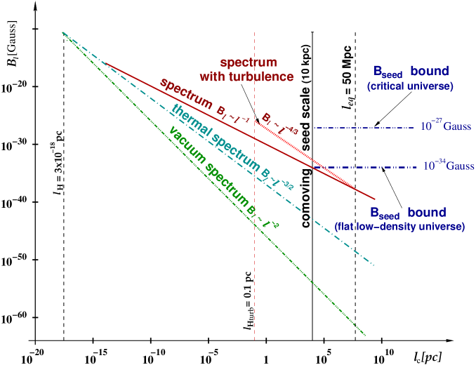
Figure 1: Comoving magnetic field spectra and relevant seed field bounds, plotted against the comoving scale $\ell_{c}$. The steepest line (dash-dot-dot-dot) depicts the (unsubtracted) vacuum spectrum $B_{\rm vac}(\ell)\propto\ell^{-2}$. At the comoving scale $\ell_{c}=10$ kpc one has $B_{\rm vac}^{\rm com}(10$ kpc$)\sim 10^{-54}$Gauss. The line of intermediate steepness (dash-dot) corresponds to the thermal spectrum $B_{\rm th}(\ell)\propto\ell^{-3/2}$, which meets the vacuum spectrum at the comoving scale $\ell_{H}$ corresponding to the Horizon at the end of inflation. The solid line is the primordial magnetic field, resulting from inflation through our mechanism, $B_{\rm rms}(\ell)\propto\ell^{\nu-3/2}\approx\ell^{-1}$, as calculated by (111). On the scale $\ell_{c}=10$ kpc we find $B_{\rm rms}^{\rm com}(10$ kpc$)\sim 10^{-34}$Gauss, i.e. about twenty orders of magnitude stronger than the value corresponding to the vacuum spectrum. This is to be compared with the dynamo bounds rescaled by a factor $10^{-4}$, corresponding to the collapse-amplification enhancement factor and the factor due to the scaling between galaxy formation and the present (see main text). These bounds read $B_{\rm seed}\geq 10^{-27}$Gauss for a Universe with critical matter density and $B_{\rm seed}\geq 10^{-34}$Gauss for a Universe dominated by dark energy (flat, low-density Universe). We also show (dotted line) the spectrum enhanced by helical turbulence (at $\ell_{c}=10$ kpc an enhancement of about 20 is obtained). Finally, we note that we expect our primordial magnetic field spectrum to depart from the $\ell^{-1}$ scaling law near the scale $\ell_{H}$ and approach approximately the thermal spectrum since $\nu\rightarrow 0$ towards the end of inflation. In that way the spectrum of our magnetic field joins the vacuum spectrum at $\ell_{H}$.

The physical momentum scales as $k\propto a^{-1}$. Thus, by scaling $k_{\rm end}$ to the present day we find,

$$k_{\rm end}=\frac{2\pi}{\ell_{c}}(\frac{T_{\rm reh}}{T_{\sc cmb}})$$ (108)

where $\ell_{c}$ is the corresponding scale of the mode in question today, $T_{\rm reh}$ is the temperature resulting from prompt reheating, $T_{\sc cmb}$ is the temperature of the CMBR at present and we have used that $a\propto T^{-1}$ at all times.

If we assume that the field remained frozen until today then, because flux conservation requires $B\propto a^{-2}$, we find that the magnitude of the magnetic field today would have been,

$$B^{\rm com}_{\rm rms}=\cos\theta_{W}\,B^{Y}_{\rm rms}(t_{\rm end})\,(\frac{T_{\sc cmb}}{T_{\rm reh}})^{2}$$ (109)

where $\cos\theta_{W}$ is introduced due to the projection of the hypercharge onto the photon at the electroweak transition according to (60).

Using (107) and (108) the above gives,

$$B^{\rm com}_{\rm rms}=\frac{1}{4}(\frac{3g_{*}}{40\pi^{2}})^{1/4}\sin(2\theta_{W})(\frac{T_{\sc cmb}}{\ell_{c}})(\frac{V_{\rm end}^{1/4}}{m_{P}})(\frac{M_{Z}}{H_{\ell}})^{2}$$ (110)

where, for prompt reheating, $V_{\rm end}\simeq(\pi^{2}/30)g_{*}T_{\rm reh}^{4}$, with $g_{*}=106.75$ being the number of relativistic degrees of freedom at the end of inflation. Putting the numbers in (110) one finds,

$$B^{\rm com}_{\rm rms}=5\times 10^{-33}\left(\frac{\mbox{1 Mpc}}{\ell_{c}}\right)\left(\frac{M_{Z}}{H_{\ell}}\right)^{2}\frac{V_{\rm end}^{1/4}}{m_{P}}\;\mbox{Gauss}$$ (111)

where $T_{\sc cmb}=2.37\times 10^{-13}$ GeV and $\sin(2\theta_{W})\approx 0.84$. The above corresponds to the spectrum of the primordial magnetic field as it would have been today were there no galactic collapse and subsequent dynamo amplification. Typically, such a field is referred to as “comoving”. The comoving spectrum of our primordial field, as given by (111) is shown in Fig. 1, where the substantial amplification compared with the vacuum spectrum is apparent.

However, the actual physical field, being frozen into the plasma, will be affected by the gravitational collapse during structure formation. Since we are interested in seeding the dynamo, we may use (110) to estimate the seed field at the time of galaxy formation. Scaling back the comoving field to galaxy formation provides an amplification factor of $(1+z_{\rm gf})^{2}$, where $z_{\rm gf}$ is the redshift that corresponds to galaxy formation. This is due to the expansion of the Universe (viewed backwards). Moreover, the collapse of matter into galaxies brings about a further amplification of magnetic fields by a factor given by the fraction of the galactic matter density to the matter density of the Universe at galaxy formation, $(\rho_{\rm gal}/\rho_{\rm gf})^{2/3}$, where $\rho_{\rm gf}=\rho_{0}(1+z_{\rm gf})^{3}$ with $\rho_{0}$ being the matter density of the Universe at present. The above result in an overall amplification factor of about $\sim 10^{4}$. Taking this into account and considering that the scale of the largest turbulent eddy corresponds to the comoving scale of about $\ell_{c}\simeq 10$ kpc before the gravitational collapse of the protogalaxy, we find,

$$B_{\rm seed}\sim 10^{-30}\mbox{Gauss}$$ (112)

where we assumed GUT-scale inflation $V_{\rm end}\sim 10^{16}$GeV and we have used that, for total number of inflationary e-foldings $\sim$ 100 we have, $(\frac{M_{Z}}{H_{\ell}})^{2}\sim 0.01$. The above seed field is sufficient to trigger the galactic dynamo in the case of a spatially-flat, dark-energy (e.g. a cosmological constant or quintessence) dominated Universe [10].

A supplementary increase in field strength is obtained if we assume that the magnetic field does not freeze into the plasma upon creation, but rather that its correlation length grows quicker than the scale factor, as is the case for helical turbulence [45]. Such a causal mechanism can only operate on a given comoving scale after this scale has reentered the horizon. One can show that the growth of correlations due to turbulent evolution leads to an additional amplification of about $(\ell_{\rm eq}/\ell_{c})^{2(1-\nu)/3}$, where $\ell_{\rm eq}\sim 50$ Mpc denotes the equal matter-radiation horizon today. For $\ell_{c}=10$ kpc and $\nu\simeq 1/2$ the amplification factor is about 20.

In the above we have assumed prompt reheating. However, it is possible that reheating may be rather inefficient and, therefore, a long-lasting process, especially in the case when the inflaton decays prominently into bosons [46]. Indeed, the reheating temperature is typically given by, $T_{\rm reh}\mbox{\raisebox{-3.87495pt}{~{}$\stackrel{{\scriptstyle\mbox{$<$}}}{{\sim}}$~{}}}\sqrt{\Gamma\,m_{P}}$, where $\Gamma$ is the perturbative decay rate of the inflaton [46][47]. If the inflaton decays into bosons then $\Gamma$ decreases with time and it is possible that the decay of the inflaton particles (inflatons) ceases before being completed leaving a small fraction of the inflatons as dark matter [46][47]. In such case $T_{\rm reh}$ may be rather low and can satisfy the gravitino constraint ($T_{\rm reh}\mbox{\raisebox{-3.87495pt}{~{}$\stackrel{{\scriptstyle\mbox{$<$}}}{{\sim}}$~{}}}10^{9}$GeV) even for GUT-scale inflation. Of course, an initial stage of preheating may increase substantially the overall efficiency of reheating [48]. However, in SUSY-HI, since $\lambda\sim h$, preheating is chaotic and likely to be also rather inefficient [49]. Finally, one can think of variations similar to “smooth Hybrid Inflation” of [35], which may achieve a rather low reheating temperature. Still, as shown in (107), the amplitude of our hypermagnetic field is, in fact, decided by the inflationary energy scale and not by the reheating temperature. Indeed, it is easy to show that, even in the case of long-lasting, inefficient, reheating the strength of our seed field at galaxy formation remains essentially unmodified, so that (111) is still applicable. Therefore, our mechanism may manage to satisfy the gravitino overproduction constraint while still able to provide a sufficiently strong seed field. Thus, our SUSY-HI inflationary model can be incorporated in a Supergravity framework without problem.

Figure 2: The formation of a magnetic field from the generation of the $Z$-boson field has to pass through the intermediate hypercharge stage similarly to light when crossing a set of orthogonal polarizers, which needs an intermediate third polarizer at some angle $\theta$ in order to go through.

At first sight, it may seem unlikely that a magnetic field is obtained from the gravitational production of the $Z$-boson field, which is orthogonal to the photon field. In fact, the situation is analogous to that of light polarizers (see Fig. 2). With two orthogonal light polarizers no light passes. When a third polarizer is inserted at an angle $\theta$ (with respect to the second polarizer) however, some of the photons do pass. The photon amplitude is reduced by $\frac{1}{2}\sin(2\theta)$, just as in the case of the $Z$-field. The main advantage of the amplification mechanism presented here is its naturalness. Indeed, no fields are required except those of the standard model and the inflaton. Moreover, the mechanism is independent of the particular model of inflation considered, but can be thought of as a generic consequence of inflationary theory itself.

An exciting possibility is that the above magnetic field can be amplified even further during preheating in an explosive resonant way. In what follows we explore this possibility using the particular model of Flipped SU(5) SUSY-HI.

5 Preheating

In addition to the growth of the superhorizon spectrum due to the breaking of the $Z$-conformal invariance in the inflationary period, the generated hypermagnetic field may be amplified more during preheating due to the backreaction of the hypercharge source current. From (40) it is evident that the growth of the amplitudes of the GUT-massive gauge fields $X^{\alpha}_{\mu}$ and $Y^{\alpha}_{\mu}$ is a prerequisite for this source current to be substantial. In Hybrid Inflation this is achieved through their mass term given by (21), which resonantly pumps energy from the GUT-Higgs field. The latter is resonantly produced at the end of inflation due to its coupling with the oscillating inflaton.

5.1 Parametric resonance in Hybrid Inflation

5.1.1 The mode equations of the scalar fields

We shall consider production of the supermassive vector bosons by parametric resonance caused by oscillations of $s$ and $\phi$. Since $s$ is a singlet and does not couple to the vector fields, the production of gauge fields is due to the GUT-Higgs field. A significant production of modes of any kind occurs only after $\phi$ and $s$ start oscillating around the bottom of the potential. Oscillations of $\phi$ are not harmonic, but to a good approximation they are periodic, with an almost constant period. This is so since the Hubble constant is small, $H=\sqrt{(\rho_{\rm inf}/3)}/m_{P}\sim\lambda M^{2}/m_{P}\sim 10^{13}$GeV, while a typical oscillation frequency is $\omega\sim\sqrt{\lambda}\,M$, where we have used (1) to estimate $\rho_{\rm inf}\equiv V(0,s_{c})$.

Since, typically, the resonant decay of a field lasts a few hundreds of oscillations, the decay time of the inflaton is $\mbox{\raisebox{-3.87495pt}{~{}$\stackrel{{\scriptstyle\mbox{$<$}}}{{\sim}}$~{}}}H^{-1}$. On these grounds one can neglect the expansion of the Universe during preheating and regard the scale factor to be approximately constant $a\simeq 1$ in agreement with the normalization (79). Therefore, the field equations (45) and (48) become,

$$\Big{(}\partial_{\tau}^{2}+h\varphi^{2}\Big{)}\sigma+\frac{\partial V_{\sigma}}{\partial\sigma} = 0$$ (113)

$$\Big{[}\partial_{\tau}^{2}+\lambda(\varphi^{2}-M^{2})+h\sigma^{2}\Big{]}\varphi=0$$ (114)

where in (114) we have ignored the backreaction of the supermassive GUT-bosons because at the onset of preheating their amplitude is negligible. In terms of the field $\bar{\varphi}=\varphi-M$ the above can be rewritten as,

$$\Big{[}\partial_{\tau}^{2}+\lambda\left(\bar{\varphi}^{2}+3\bar{\varphi}M+2M^{2}\right)+h\sigma^{2}\Big{]}\bar{\varphi}+h\sigma^{2}M = 0$$

$$\Big{[}\partial_{\tau}^{2}+h(\bar{\varphi}^{2}+2\bar{\varphi}M+M^{2})\Big{]}\sigma = 0.$$ (115)

where we have ignored the term $\frac{\partial V_{\sigma}}{\partial\sigma}$ since the slope of the $V_{\sigma}$ potential is negligible compared to the interaction term. The solutions to these equations are damped periodic oscillatory functions which in general have the following form,

$$\bar{\varphi} = \varphi_{0}P_{\varphi}(\omega_{\varphi}\tau)$$

$$\sigma = \sigma_{0}P_{\sigma}(\omega_{\sigma}\tau),$$ (116)

where $P_{\varphi}(x+2\pi)=P_{\varphi}(x)$, and $P_{\sigma}(x+2\pi)=P_{\sigma}(x)$, max$\{|P_{\varphi}|\}=1$ and max$\{|P_{\sigma}|\}=1$, and $\varphi_{0}$ and $\sigma_{0}$ are the amplitudes of oscillations, which are in principle time-dependent since $\varphi$ and $\sigma$ eventually decay and redshift.

The corresponding mode equations can be obtained with Fourier transform. The result is,

$$\Big{[}\partial_{\tau}^{2}+k^{2}+\lambda\left(3\bar{\varphi}^{2}+6\bar{\varphi}M+2M^{2}\right)+h\sigma^{2}\Big{]}\varphi_{k}+2h\sigma(\bar{\varphi}+M)\sigma_{k} = 0\qquad$$ (117)

$$\Big{[}\partial_{\tau}^{2}+k^{2}+h(\bar{\varphi}^{2}+2\bar{\varphi}M+M^{2})\Big{]}\sigma_{k}+2h\sigma(\bar{\varphi}+M)\varphi_{k} = 0$$ (118)

By making use of $\langle\bar{\varphi}^{2}\rangle=\varphi_{0}^{2}/2$ and $\langle\sigma^{2}\rangle=\sigma_{0}^{2}/2$, we can easily estimate the effective masses of the modes to be,

$$m_{\varphi}^{2} = 2\lambda\left(M^{2}+\frac{3}{4}\varphi_{0}^{2}\right)+\frac{1}{2}h\sigma_{0}^{2}\simeq 4\lambda M^{2}$$

$$m_{\sigma}^{2} = h\left(M^{2}+\frac{1}{2}\varphi_{0}^{2}\right)\simeq\frac{3}{2}hM^{2}$$

so that the dispersion relations read,

$$\omega_{\varphi}^{2} = k^{2}+2\lambda\left(M^{2}+\frac{3}{4}\varphi_{0}^{2}\right)+\frac{1}{2}h\sigma_{0}^{2}\simeq k^{2}+4\lambda M^{2}$$

$$\omega_{\sigma}^{2} = k^{2}+h\left(M^{2}+\frac{1}{2}\varphi_{0}^{2}\right)\simeq k^{2}+\frac{3}{2}hM^{2}$$

where $\varphi_{0}^{2}\simeq M$ and $\sigma_{0}^{2}\simeq s_{c}^{2}=(\lambda/h)M^{2}$. Note that the effective mass of the $\bar{\varphi}$ modes is a factor of $\sqrt{2}$ larger than the Higgs mass $M_{H}=\sqrt{2\lambda}\,M$.

We need to investigate whether the mode equations (117) and (118) result in a broad or narrow resonance, and also whether the leading (broad) resonance is active. To do that we have to consider the quality factors $q$ for the mode equations and then compare them to the effective masses (LABEL:effmasses).

5.1.2 The characteristics of the resonance

The generic form for a resonance equation is

$$\frac{d^{2}\psi_{k}}{d^{2}\varpi}+\Big{[}A_{k}+\sum_{i}2q_{i}P_{i}(\varpi)\Big{]}\psi_{k}=0\hskip 28.45274pt\mbox{where}\hskip 28.45274ptA_{k}=\frac{m_{\psi\,\rm eff}^{2}+k^{2}}{\omega_{\varphi}^{2}}=1$$ (121)

and $q_{i}$ are the quality factors with oscillating functions $P_{i}(\varpi)$ ($\langle P_{i}\rangle_{\varpi}=0$, max${}_{x}\{P_{i}\}=1$) whose period is either $\pi$ or $2\pi$, and $\varpi\equiv\omega_{\varphi}\tau$ is the rescaled time variable. In the Mathieu case, $P_{i}=\cos(2\varpi)$. Some of the references where one can find instability charts, which are plots of the Floquet exponent $\mu$ in terms of $q$ and $A$, are listed in [50][46][47].

Consider first the quality factors for (117),

$$q_{\varphi\,1}=\frac{3\lambda\varphi_{0}^{2}}{4\omega_{\varphi}^{2}}\sim\frac{3}{16}\qquad q_{\varphi\,2}=\frac{6\lambda M\varphi_{0}}{2\omega_{\varphi}^{2}}\sim\frac{3}{4}\qquad q^{\prime}_{\sigma\,1}=\frac{2hM\sigma_{0}}{2\omega_{\varphi}^{2}}\sim\frac{1}{4}\sqrt{\frac{h}{\lambda}}$$ (122)

Since $\omega_{\varphi}^{2}\simeq 4\lambda M^{2}$, we conclude that all the quality factors of (117) are generically of the order unity. The quality factors for (118) are on the other hand

$$q_{\sigma\,1}=\frac{h\varphi_{0}^{2}}{4\omega_{\varphi}^{2}}\sim\frac{1}{16}\frac{h}{\lambda}\qquad q_{\sigma\,2}=\frac{2hM\varphi_{0}}{2\omega_{\varphi}^{2}}\sim\frac{1}{4}\frac{h}{\lambda}\qquad q^{\prime}_{\varphi\,1}=\frac{2hM\sigma_{0}}{2\omega_{\varphi}^{2}}\sim\frac{1}{4}\sqrt{\frac{h}{\lambda}}$$ (123)

so that they are typically smaller than the quality factors (122) of (117). Further we can compute

$$A_{\varphi}(k\!=\!0) = \frac{m_{\varphi}^{2}}{\omega_{\varphi}^{2}}=1\sim\frac{4}{3}q_{\varphi\,2}$$

$$A_{\sigma}(k\!=\!0) = \frac{m_{\sigma,\bar{\varphi}=0}^{2}}{\omega_{\varphi}^{2}}=\frac{1}{4}\frac{h}{\lambda}\sim q_{\sigma\,2}$$ (124)

which then determines onto which resonance the field can decay. Note that since the position of the first resonance is at $A\sim 1$ for $q<1$, we conclude that the $\varphi$ field tends to decay into the first resonance such that the infrared superhorizon modes get populated (see figure in [46]) with $\mu\sim 0.3$ or smaller. A similar statement applies to the $\sigma$ field.

The strength of the broad resonances may be as large as $\mu\sim 0.2$ along the $A=2q$ line, and becomes rapidly stronger at smaller values of $A$, i.e. $A<2q$ (cf. Eq. (7) in [50]). Even if the field can decay only into the second available resonance, the strength is expected to be of the order $\mu_{2}\sim 0.04$, just like it is in the case of the chaotic inflation with a quartic scalar interaction term, which decays into the second resonance.

Regarding the $\sigma$ field, depending on the choice of the couplings, $q_{\sigma\,2}$ can be larger or smaller then unity. Generically, however, we expect that $\lambda\sim h$, and hence $q_{\sigma\,2}$ is typically of the order (but smaller then) unity. In SUSY-HI we have $\lambda=2h$ and, therefore, $q_{\sigma\,2}\simeq\frac{1}{8}<1$.

In the above, by taking $a\simeq 1$ we have ignored Hubble damping. It is known that the latter, in fact, results in stochastic resonant amplification, in the sense that the action of the damping term may be positive or negative on occasion, depending on whether the amplitude of the oscillating fields is increasing or decreasing. However, as has been shown in [47][48], the net effect of such a term is, in fact, in favor of resonant production.

This analysis has not covered the mixing terms in (117) and (118). Numerical simulations done by the authors of [50] indicate that these terms typically cannot prevent resonant decay, and in some cases can enhance it.

5.2 Resonant production of massive vector bosons

The field equations for the supermassive GUT-bosons are (23) and (24), while (28) is the one of for the $V$-boson. The resonant production of the massive bosons is due to the fact that their equations of motion are of harmonic form with frequencies given by their oscillating mass term.

5.2.1 The parametric resonance equations

At the onset of preheating we may ignore the backreaction source current because the initial amplitude of the massive bosons is negligible. Later on the source current contributes additionally to the production of the massive bosons.

Let us concentrate on (23) first. Proceeding in a similar manner as in 4.1 we obtain for the longitudinal and transverse modes,

$$\Big{[}(\partial_{\tau}^{2}+k^{2}+M_{XY}^{2})+\frac{2(\partial_{\tau}\ln M_{XY})k^{2}}{k^{2}+M_{XY}^{2}}\partial_{\tau}\Big{]}\mbox{\boldmath$\cal X$}^{\alpha\parallel} = 0$$ (125)

$$\Big{(}\partial_{\tau}^{2}+k^{2}+M_{XY}^{2}\Big{)}\mbox{\boldmath$\cal X$}^{\alpha\perp} = 0$$ (126)

where

$$X_{\mu}^{\alpha}(\mbox{\boldmath$x$},\tau)=\int\frac{d^{3}k}{(2\pi)^{3}}\,{\cal X}_{\mu}^{\alpha}(\mbox{\boldmath\bf$k$},\tau)\exp(i\mbox{\boldmath\bf$k\cdot x$})$$ (127)

Recalling that $\varphi=M+\varphi_{0}P_{\varphi}(\omega_{\varphi}\tau)$ and using (21) we can find the effective mass ${\cal M}_{XY}$ of $X_{\mu}^{\alpha}$ during preheating to be,

$$M_{XY}^{2}=\frac{1}{2}g^{2}(M^{2}+\varphi_{0}^{2}P_{\varphi}^{2}+2M\varphi_{0}P_{\varphi})\Rightarrow{\cal M}_{XY}^{2}=\frac{1}{2}g^{2}M^{2}\Big{[}1+\frac{1}{2}(\frac{\varphi_{0}}{M})^{2}\Big{]}\simeq\frac{3}{4}g^{2}M^{2}$$ (128)

where we used that $\langle P_{\varphi}^{2}\rangle_{\tau}=1/2$ and $\langle P_{\varphi}\rangle_{\tau}=0$. Rescaling the time as $\omega_{\varphi}\tau\rightarrow\varpi$, the equations (125) and (126) can be recast as,

$$\left[\Big{(}\partial_{\varpi}^{2}+\frac{k^{2}+M_{XY}^{2}}{\omega_{\varphi}^{2}}\Big{)}+\frac{2(\partial_{\varpi}\ln M_{XY})k^{2}}{k^{2}+M_{XY}^{2}}\partial_{\varpi}\right]\mbox{\boldmath$\cal X$}^{\alpha\parallel} = 0$$ (129)

$$\Big{(}\partial_{\varpi}^{2}+\frac{k^{2}+M_{XY}^{2}}{\omega_{\varphi}^{2}}\Big{)}\mbox{\boldmath$\cal X$}^{\alpha\perp} = 0$$ (130)

Now, it easy to show that, in the above, we have,

$$\frac{k^{2}+M_{XY}^{2}}{\omega_{\varphi}^{2}}=\frac{k^{2}+{\cal M}_{XY}^{2}}{\omega_{\varphi}^{2}}+\frac{g^{2}M^{2}}{2\omega_{\varphi}^{2}}\Big{[}\frac{1}{2}(\frac{\varphi_{0}}{M})^{2}\hat{P}_{\varphi}+2\frac{\varphi_{0}}{M}P_{\varphi}\Big{]}$$ (131)

where $\hat{P}_{\varphi}=2P_{\varphi}^{2}-1$ is a periodic function of $\varpi$ with frequency $\hat{\omega}_{\varphi}=2\omega_{\varphi}$ and max{$|\hat{P}_{\varphi}|$}=1. Each of the above equations contains two resonant channels with the $q$-factors,

$$q_{1} = \frac{g^{2}M^{2}}{2\omega_{\varphi}^{2}}\frac{\varphi_{0}}{M}\simeq\frac{g^{2}}{8\lambda}\qquad$$

$$q_{2} = \frac{g^{2}M^{2}}{8\omega_{\varphi}^{2}}(\frac{\varphi_{0}}{M})^{2}\simeq\frac{g^{2}}{32\lambda}\simeq\frac{1}{4}q_{1}$$

$$A_{k=0} = \frac{{\cal M}_{XY}^{2}}{\omega_{\varphi}^{2}}\simeq\frac{3g^{2}}{16\lambda}\simeq\frac{3}{2}q_{1}\simeq 6q_{2}$$ (132)

This implies that, provided $q_{1,2}\mbox{\raisebox{-3.87495pt}{~{}$\stackrel{{\scriptstyle\mbox{$>$}}}{{\sim}}$~{}}}1/2$, the $q_{1}$-resonance is efficient in amplifying gauge fields, while the $q_{2}$-resonance is inefficient. In fact when $A_{k=0}<2q$ {$A_{k=0}>2q$} the growth rate of the field grows {decreases} with increasing $q$ [50], implying that for $A_{k=0}\simeq\frac{3}{2}q_{1}$ the resonance becomes stronger as $q_{1}$ increases. For example, one enters the first broad resonance at about $q_{1}\simeq 1/2$ and exits it at about $q_{1}\simeq 3$.

When compared with the transverse equation (130), the longitudinal equation (129) contains an additional ‘damping’ term. The sign of the ‘damping’ coefficient $\partial_{\varpi}\ln M_{XY}=\partial_{\varpi}P_{\varphi}/P_{\varphi}$ may be either positive or negative, resulting in damping or growth, respectively. Since the positive and negative parts are symmetrically and evenly distributed, we expect that the growth wins over the damping, just as it is in the case of stochastic resonance [48]. As a consequence, the longitudinal modes grow faster than the transverse modes. Large longitudinal amplitudes can be mediated to the transverse modes through scatterings. We do not consider here possible physical consequences of these processes.

Similar results are obtained for the $Y^{\alpha}_{\mu}$ and the $V_{\mu}$ bosons, substituting, in the latter case $M_{XY}\rightarrow M_{V}$ or equivalently $g\rightarrow 2\sqrt{(6/5)}\,g/\cos\Theta$.

5.2.2 The amplitudes of the massive vector bosons

In order for the backreaction to stop resonant production of the massive gauge fields, the induced (Hartree) mass must be larger than about the mass of the Higgs boson, since this is the typical resonance scale. This can be argued as follows. The shift in $A$ required to switch off the leading resonance is of the order $\delta A\sim 0.5$. This cannot be mediated by the $\varphi$-field modes, since the maximum possible expectation value is $\langle(\delta\varphi)^{2}\rangle_{\rm max}\sim M^{2}$, resulting in $\delta A=\delta{\cal M}_{XY}^{2}/\omega_{\varphi}^{2}\sim g^{2}/16\lambda$, which is typically not sufficient to shut down the resonance. Moreover, the inflaton does not help, since it does not couple to the vector bosons.

There are however cubic terms in the source current, which have been neglected in (130) and which may shut down the resonance. The cubic source current terms can be obtained from (25). Similarily to (3.3), for the supermassive GUT-bosons we have,

$$(J^{\nu}_{\xi\alpha})^{\rm cubic}_{XY}=g^{2}g^{\mu\rho}g^{\nu\sigma}Re[(\mbox{$\Omega$}_{\mu})_{\xi i}(\mbox{$\Omega$}_{\rho})_{ij}(\mbox{$\Omega$}_{\sigma})_{j\alpha}-(\rho\leftrightarrow\sigma)]$$ (133)

where $\xi=4,5$ and $\alpha=1,2,3$. In view of (13), (133) can be written schematically as

$$J^{\rm cubic}_{XY}\sim g^{2}(XXX+WWX+WVX+VVX),$$ (134)

where $X$ denotes the supermassive GUT-bosons $X^{\alpha}_{\mu}$ and $Y^{\alpha}_{\mu}$, $W$ denotes the electroweak gauge bosons $W^{\pm}_{\mu},\,Y_{\mu}$, which are gravitationally produced in inflation as shown in Sec. 4, and $V$ is the massive $V$-boson. Note that the contribution from the $G$-bosons of SU(3)_c is negligible because they are neither produced gravitationally in inflation, nor are they generated during preheating, since they do not couple to any Higgs field. Thus, a typical contribution of the backreaction current to the mass of the $X^{\alpha}_{\mu},Y^{\alpha}_{\mu}$ fields, coming from their resonant production, is of the form

$$\delta M^{2}_{XY}\sim g^{2}(\langle X^{2}\rangle+\langle V^{2}\rangle)$$ (135)

Similarly, for $V_{\mu}$ we have from (28) that $J^{\nu}_{V}=-\sqrt{\frac{5}{12}}\,\cos\Theta J_{Y}^{\nu}$ so that the cubic term contribution is given by (34) to be,

$$J^{\rm cubic}_{V}\sim\frac{5}{6}\,g^{2}XXV$$ (136)

Hence, the contribution of the backreaction current to the mass of the $V_{\mu}$ is,

$$\delta M^{2}_{V}\sim\frac{5}{6}\,g^{2}\langle X^{2}\rangle$$ (137)

In order to get the first resonance to shut down, one requires $\delta M^{2}\sim M_{H}^{2}=2\lambda M^{2}$. Hence, the energy stored in the $X$ and $V$ fields is then of the order,

$$\rho_{XV}\sim g^{2}(\langle X^{2}\rangle^{2}+\langle V^{2}\rangle^{2})\sim\frac{\lambda^{2}}{g^{2}}M^{4}\sim\frac{\lambda}{g^{2}}\rho_{\rm inf}$$ (138)

Since $\lambda\sim 1$ we conclude that the resonance shuts down only when most of the energy is in the massive gauge field modes. In other words, the resonance is efficient until a significant fraction of the inflaton’s energy decays. Then, as the oscillating amplitude of $\varphi$ decreases, one enters the narrow resonance and the decay slows down. This is just like the case of two scalar fields with $q\sim 1$, and also the one field case, where also $q\sim 1$. One is then left with the condensates of the gauge fields whose amplitude can be estimated to be,

$$|X^{\alpha}_{\mu}|,|Y^{\alpha}_{\mu}|,|V_{\mu}|\sim g_{*}^{-1/4}\frac{M_{H}}{g}\sim 0.1M_{H}$$ (139)

where $g_{*}\mbox{\raisebox{-3.87495pt}{~{}$\stackrel{{\scriptstyle\mbox{$<$}}}{{\sim}}$~{}}}100$ is the effective number of degrees of freedom produced by the resonance.

5.3 The hypercharge field at preheating

In a similar manner as for the supermassive GUT-bosons one finds from (29) that the hypercharge transverse mode equation is,

$$\Big{(}\partial_{\tau}^{2}+k^{2}\Big{)}\mbox{\boldmath$\cal Y$}^{\perp}=\sqrt{\mbox{$\frac{5}{12}$}}\sin\Theta\mbox{\boldmath$\cal J$}_{\!Y}^{\perp}$$ (140)

where

$$J_{Y}^{\nu}(\mbox{\boldmath$x$},\tau)\!=\!\!\int\!\frac{d^{3}k}{(2\pi)^{3}}\,{\cal J}_{\!Y}^{\nu}(\mbox{\boldmath\bf$k$},\tau)\exp(i\mbox{\boldmath\bf$k\cdot x$}) Y^{\nu}(\mbox{\boldmath$x$},\tau)\!=\!\!\int\!\frac{d^{3}k}{(2\pi)^{3}}\,{\cal Y}^{\nu}(\mbox{\boldmath\bf$k$},\tau)\exp(i\mbox{\boldmath\bf$k\cdot x$})$$ and (141)

and we have used the current conservation equation, $\partial_{\tau}({\cal J}_{Y})_{\tau}=i\mbox{\boldmath$k\cdot\cal J$}_{\!Y}$.

Using the Hartree approximation, as shown in the appendix A.1, and also in view of (38) we can recast (140) as,

$$\left\{\partial_{\tau}^{2}+k^{2}+6\,\bar{g}_{Y}^{2}\Big{[}\mbox{\normalsize$\frac{2}{3}$}\langle|\mbox{\boldmath$X$}|^{2}\rangle_{{}_{V}}-\langle|X_{\tau}|^{2}\rangle_{{}_{V}}\Big{]}\right\}\mbox{\boldmath${\cal Y}$}^{\perp}=-6\,\bar{g}_{Y}^{2}\cot\Theta\Big{[}\mbox{\normalsize$\frac{2}{3}$}\langle|\mbox{\boldmath$X$}|^{2}\rangle_{{}_{V}}-\langle|X_{\tau}|^{2}\rangle_{{}_{V}}\Big{]}\mbox{\boldmath${\cal V}$}^{\perp}$$ (142)

where $\bar{g}_{Y}^{2}\equiv\frac{5}{6}g_{Y}^{2}$ and $X_{\mu}$ stands for all the 6 the supermassive GUT-bosons $X_{\mu}^{\alpha},Y_{\mu}^{\alpha}$ with,

$$\langle|\mbox{\boldmath$X$}|^{2}\rangle_{{}_{V}} = \frac{1}{V}\int\frac{k^{2}dk}{2\pi^{2}}\mbox{\boldmath${\cal X}$}(\mbox{\boldmath$k$},\tau)\mbox{\boldmath${\cal X}$}(-\mbox{\boldmath$k$},\tau)\;\;\;\,\simeq\;\;\frac{1}{V}\int\frac{k^{2}dk}{2\pi^{2}}|\mbox{\boldmath${\cal X}$}(k,\tau)|^{2}$$ (143)

$$\langle|X_{\tau}|^{2}\rangle_{{}_{V}} = \frac{1}{V}\int\frac{k^{2}dk}{2\pi^{2}}{\cal X}_{\tau}(\mbox{\boldmath$k$},\tau){\cal X}_{\tau}(-\mbox{\boldmath$k$},\tau)\;\;\simeq\;\;\frac{1}{V}\int\frac{k^{2}dk}{2\pi^{2}}[{\cal X}_{\tau}(k,\tau)]^{2}$$

and also [cf. (73) and (76)],

$$X_{\rm rms}^{2}\equiv\frac{2}{3}\langle|\mbox{\boldmath$X$}|^{2}\rangle_{{}_{V}}-\langle|X_{\tau}|^{2}\rangle_{{}_{V}}=\frac{1}{V}\int\frac{k^{2}dk}{2\pi^{2}}\left\{\frac{2}{3}[\mbox{\boldmath${\cal X}$}(\tau)]^{2}+\frac{k^{2}[\partial_{\tau}\mbox{\boldmath${\cal X}$}^{\parallel}(\tau)]^{2}}{k^{2}+M_{XY}^{2}}\right\}$$ (144)

We shall now investigate whether the hypercharge field (142) may undergo resonant amplification at preheating. Since the supermassive GUT-bosons are mainly produced at preheating, the dominant contribution to $X_{\rm rms}^{2}$ comes from the resonant modes that initially oscillate in phase [50], which in principle may drive resonant amplification of the hypercharge. We now discuss the necessary conditions required for this indirect resonance to be operative.

At early times in preheating the Hartree terms $X_{\rm rms}^{2}$ are small, so that the hypercharge bosons grow through (inefficient) narrow parametric resonance [51]. When the oscillatory component of $X_{\rm rms}^{2}$ becomes of the order $\omega_{\varphi}^{2}$ however, the hypercharge resonance can become broad [46]. Since the hypercharge field has an infrared spectrum that is already amplified in inflation, while the $V$-boson spectrum is that of the Minkowski vacuum, when compared with the $X^{2}V$-term, the $X^{2}Y$-term is expected to dominate the resonant growth on superhorizon scales. Therefore, we may write,

$$\mbox{\boldmath$\cal J$}_{\!Y}^{\perp}(\tau)\simeq-6\sqrt{2}\,g\bar{g}_{Y}X_{\rm rms}^{2}\mbox{\boldmath${\cal Y}$}^{\perp}(\tau)$$ (145)

so that (142) simplifies to

$$\frac{d^{2}\mbox{\boldmath$\cal Y$}^{\perp}}{d\tau^{2}}+\left(k^{2}+6\,\bar{g}_{Y}^{2}X_{\rm rms}^{2}\right)\mbox{\boldmath$\cal Y$}^{\perp}\simeq 0$$ (146)

Now, $X_{\rm rms}^{2}$ can be conveniently split into the slowly growing and oscillatory contributions as follows:

$$X_{\rm rms}^{2}=X_{0}^{2}(\tau)+X_{\rm osc}^{2}[1+P_{X}(\tau)]$$ (147)

where $P_{X}(\tau)$ is a periodic function with period $\sim\pi/\omega_{\varphi}$ such that $\langle P_{X}(\tau)\rangle_{\tau}=0$ and $\langle P_{X}^{2}(\tau)\rangle_{\tau}=1/2$, and

$$X_{0}^{2}(\tau)=X_{\rm vac}^{2}\left(e^{2\mu_{0}\omega_{\varphi}\tau}-1\right),\qquad X_{\rm osc}^{2}(\tau)=X_{\rm vac}^{2}\left(e^{2\mu_{X}\omega_{\varphi}\tau}-1\right)$$ (148)

where $\mu_{X}$ denotes the relevant resonant growth rate of the supermassive GUT-boson fields $X$, and $\mu_{0}$ is the growth rate of the constant contribution to the $X$-field mass induced by the inelastic scatterings. Also, we have subtracted the vacuum contribution $X_{\rm vac}^{2}\sim k_{\rm res}^{2}$, with $k_{\rm res}^{2}$ being the typical resonant momentum. Provided $\mu_{0}<\mu_{X}$, or equivalently $X_{0}<X_{\rm osc}$, the hypercharge grows resonantly. The amount of available energy $\rho_{\rm inf}\simeq\lambda M^{4}/4$ results in the following upper bound,

$$\frac{1}{2}{\cal M}_{XY}^{2}X_{\rm rms}^{2}\mbox{\raisebox{-3.87495pt}{~{}$\stackrel{{\scriptstyle\mbox{$<$}}}{{\sim}}$~{}}}\frac{1}{8}M_{H}^{2}M^{2}$$ (149)

or equivalently [cf. (128)]

$$X_{\rm rms}^{2}\mbox{\raisebox{-3.87495pt}{~{}$\stackrel{{\scriptstyle\mbox{$<$}}}{{\sim}}$~{}}}\frac{2\lambda}{3g^{2}}M^{2}$$ (150)

where ${\cal M}_{XY}^{2}\simeq 3g^{2}M^{2}/4$ and $M_{H}^{2}=2\lambda M^{2}$. This is in agreement with (139) and implies the following bound for the quality factor of the hypercharge resonance,

$$q_{Y}=\frac{6\,\bar{g}_{Y}^{2}X_{\rm osc}^{2}}{2\omega_{\varphi}^{2}}\mbox{\raisebox{-3.87495pt}{~{}$\stackrel{{\scriptstyle\mbox{$<$}}}{{\sim}}$~{}}}\frac{5}{12}\sin^{2}\Theta<0.4$$ (151)

where $\sin\Theta=g_{Y}/g$. Since significant resonant amplification of the hypercharge on superhorizon scales may occur without tuning only when $q_{Y}\mbox{\raisebox{-3.87495pt}{~{}$\stackrel{{\scriptstyle\mbox{$>$}}}{{\sim}}$~{}}}1/2$, we conclude that the inflationary spectrum of the hypercharge gauge bosons is hardly amplified by parametric resonance.

6 Conclusions

We have presented a mechanism of primordial magnetic field generation based on the breaking of conformal invariance of the $Z$-boson field during inflation. The mechanism is generic and independent of inflationary model as long as the reheating temperature is higher than the electroweak scale. This is because our mechanism requires a phase of electroweak unification to “channel” the generated superhorizon $Z$-boson spectrum into the photon, through the hypercharge field.

The conformal invariance of $Z$ is naturally broken due to its standard-model coupling with the electroweak Higgs-field. The latter, during inflation, develops a condensate comparable to the one of the inflaton field itself resulting in a non-zero, but small, mass for the $Z$-boson field. Conformal invariance breakdown results in gravitational production of the $Z$-field on superhorizon scales. We have computed the relevant superhorizon spectrum and found that it is almost scale invariant. At the end of inflation reheating restores the electroweak symmetry and the $Z$-spectrum is converted into a hypercharge spectrum (the photon’s contribution being negligible), which, due to the stochastic nature of the original $Z$-fluctuations, gives rise to a superhorizon hypermagnetic field that freezes into the reheated plasma. We have calculated the spectrum of the rms value of the hypermagnetic field and found that it is of the form $B_{\rm rms}\propto 1/\ell$ as shown in Fig. 1. In a similar way non-Abelian $W$-fields are also generated but their associated magnetic fields are screened due to the existence of a magnetic mass of non-perturbative nature, which stems from their self-interaction. During the radiation era the hypermagnetic field evolves satisfying flux conservation. At the electroweak phase transition it is transformed into a regular magnetic field. When scaled until galaxy formation, this magnetic field is found to be sufficient to trigger the galactic dynamo and explain the observed galactic magnetic fields in the case of a spatially-flat, dark-energy dominated Universe with GUT-scale inflation.

The beauty of our mechanism, apart from being independent of the inflationary model, lies in that it does not, unlike most proposed mechanisms, require the explicit introduction of conformal invariance breaking terms in the Lagrangian or any exotic fields other than the ones of the standard model and the inflaton field. Moreover, we do not have to specify a particular GUT group, or involve grand unification in any way.

An intriguing possibility was that our magnetic field could be further amplified during preheating. In order to study this we considered a (supersymmetric) hybrid inflationary model and grand unification under Flipped SU(5), both well motivated. However, we have found that preheating amplification is probably negligible since the hypercharge field is amplified only via indirect narrow resonance which turns out to be rather inefficient. Still, a better (possibly numerical) treatment of the magnetic field at preheating is probably necessary to provide an adequate understanding of its behavior. Such treatment should, in principle, address issues such as the conductivity of the newly created plasma or the fate of the hyperelectric field.

In particular, the behavior of the conductivity during preheating may inhibit our hypermagnetic field. However, an analytic treatment of this issue is rather complex and beyond the scope of the present article and numerical studies are inconclusive. It seems that the behavior of the conductivity (spatial distribution and growth rate) is highly non-trivial, non-perturbative and model dependent [22]. It has been shown however, that the appearance of conductivity in preheating does not necessarily inhibit the growth or the existence of (hyper)magnetic fields but may allow substantial amplification [22][53]. This is certainly an issue that deserves further investigation.

In summary, we have presented a natural mechanism for magnetogenesis by inflation which may be an explanation for galactic magnetic fields.

Acknowledgements

Support for K.D. was provided by DGICYT grant PB98-0693 and by the European Union under contract HPRN-CT00-00148; O.T. wishes to thank the Theoretical Physics Group at Imperial College for a Visiting Fellowship. We gratefully acknowledge travel support by the U.K. PPARC. This work is supported in part by PPARC.

Appendix A The Hartree approximation

In this appendix we discuss the use of the Hartree approximation in the computation of scalar and gauge fields. This approximation is applicable in this case mainly due to the classicallity of the superhorizon modes and also since the typical value of the quality factor $q$ of the parametric resonance is about one or smaller, essentially until the field grows to its maximum value.

The Hartree approximation takes account of elastic scatterings only, which do not change the momenta of incoming particles, and it models the dynamics well when 2-to-2 scatterings are the only ones that are relevant. This is indeed so at the early stages of preheating, as is known from exact classical simulations (e.g. of the scalar theory). When thermalization begins, inelastic scatterings, which include 2-to-4, etc., become important. They combine the infrared modes into more energetic ones, as it is required by the thermalization process, because particles produced by parametric resonance are more infrared in comparison to a thermal distribution. The Hartree approximation breaks down after a significant fraction of the inflaton’s energy has decayed.

The Hartree approximation consists essentially in replacing a product of two fields (in an equation of motion) with the spatial average as follows,

$$A(\mbox{\boldmath$x$},t)\,B(\mbox{\boldmath$x$},t)\rightarrow\langle A(\mbox{\boldmath$x$},t)\,B(\mbox{\boldmath$x$},t)\rangle_{{}_{V}}=\tilde{A}\tilde{B}+\langle\delta A(\mbox{\boldmath$x$},t)\,\delta B(\mbox{\boldmath$x$},t)\rangle_{{}_{V}}$$ (152)

where $\tilde{A}$ and $\tilde{B}$ denote the zero modes defined as $\tilde{A}\equiv\langle A(\mbox{\boldmath$x$},t)\rangle_{{}_{V}}$, $\tilde{B}\equiv\langle B(\mbox{\boldmath$x$},t)\rangle_{{}_{V}}$ and also
$\delta A(\mbox{\boldmath$x$},t)=A(\mbox{\boldmath$x$},t)-\tilde{A}$, $\delta B(\mbox{\boldmath$x$},t)=B(\mbox{\boldmath$x$},t)-\tilde{B}$, with the volume averages being defined as,

$$\langle\delta A(\mbox{\boldmath$x$},t)\,\delta B(\mbox{\boldmath$x$},t)\rangle_{{}_{V}} \equiv \frac{1}{V}\int d^{3}x\,\delta A(\mbox{\boldmath$x$},t)\,\delta B(\mbox{\boldmath$x$},t)\;=\;\frac{1}{V}\int^{\prime}\frac{d^{3}k}{(2\pi)^{3}}{\cal A}(\mbox{\boldmath$k$},t)\,{\cal B}(-\mbox{\boldmath$k$},t)$$

$$\tilde{A} \equiv \frac{1}{V}\int d^{3}x\,A(\mbox{\boldmath$x$},t)=\frac{1}{V}\;{\cal A}(\mbox{\boldmath$k$}\!=\!0,t)$$ (153)

In these definitions the volume $V$ is defined by the following discretized version of the momentum integral

$$\int\frac{d^{3}k}{(2\pi)^{3}}\rightarrow\frac{1}{V}\sum_{\mbox{\scriptsize\boldmath$k$}}$$ (154)

The prime in the momentum integral indicates that the zero mode should be taken out of the integral. The zero modes require special care, since they may become macroscopic, leading to a condensate.

A.1 Hypercharge source current

Let us employ the Hartree approximation in computing the source current of the hypercharge which is shown explicitly in (38). In the spirit of our approximation, we shall neglect the terms in which the zero modes figure incoherently in quadratic or cubic combinations. This means that at this point we shall take account only of those nonlinear contributions from the zero modes which oscillate coherently in time.

Some of the remaining terms are composed of the fields which have incoherent phases in different points in space, so that, when averaged over space, they vanish. Including these terms is strictly speaking beyond the Hartree approximation. Therefore, to first approximation we keep only the terms that contribute to the genuine Hartree approximation, which are the terms that oscillate coherently in space and time, since they dominate the resonant production.

Consider first the derivative terms of the source current in (38),

$$-\mbox{\normalsize$\sqrt{\frac{5}{12}}$}\,\sin\Theta\,J_{Y}^{\nu}[X\partial X] \equiv -\;\bar{g}_{Y}\,\mbox{Im}\Big{\{}[\partial_{\mu}+(\partial_{\mu}\ln\sqrt{-D_{g}})]g^{\mu\rho}g^{\nu\sigma}(X^{\alpha}_{\rho}\overline{X}^{\alpha}_{\sigma}+Y^{\alpha}_{\rho}\overline{Y}^{\alpha}_{\sigma})\,+$$

$$+\;g^{\mu\rho}g^{\nu\sigma}[X^{\alpha}_{\mu}\partial_{\rho}\overline{X}^{\alpha}_{\sigma}+Y^{\alpha}_{\mu}\partial_{\rho}\overline{Y}^{\alpha}_{\sigma}-(\rho\leftrightarrow\sigma)]\Big{\}}$$

In CFRW with $a\simeq 1$ the above may be written as,

$$-\mbox{\normalsize$\sqrt{\frac{5}{12}}$}\sin\Theta J^{Y}_{\rho}[X\partial X]=\!-\bar{g}_{Y}\eta^{\mu\sigma}\mbox{Im}\Big{\{}\partial_{\mu}(X^{\alpha}_{\rho}\overline{X}^{\alpha}_{\sigma}+Y^{\alpha}_{\rho}\overline{Y}^{\alpha}_{\sigma})+X^{\alpha}_{\mu}(\partial_{\rho}\overline{X}^{\alpha}_{\sigma}-\partial_{\sigma}\overline{X}^{\alpha}_{\rho})+Y^{\alpha}_{\mu}(\partial_{\rho}\overline{Y}^{\alpha}_{\sigma}-\partial_{\sigma}\overline{Y}^{\alpha}_{\rho})\Big{\}}$$ (156)

Hartree averaged the terms in the above are of the form,

$$\langle X^{\alpha}_{\mu}\partial_{0}\overline{X}^{\alpha}_{\sigma}\rangle_{{}_{V}}\equiv\frac{1}{V}\int d^{3}\!x\,X^{\alpha}_{\mu}\partial_{0}\overline{X}^{\alpha}_{\sigma} = \frac{1}{V}\int\frac{d^{3}k}{(2\pi)^{3}}\,{\cal X}^{\alpha}_{\mu}(\mbox{\boldmath$k$},\tau)\,\partial_{\tau}\overline{{\cal X}}^{\alpha}_{\sigma}(\mbox{\boldmath$k$},\tau)$$

$$\langle X^{\alpha}_{\mu}\partial_{i}\overline{X}^{\alpha}_{\sigma}\rangle_{{}_{V}}\equiv\frac{1}{V}\int d^{3}\!x\,X^{\alpha}_{\mu}\partial_{i}\overline{X}^{\alpha}_{\sigma} = \frac{1}{V}\int\frac{d^{3}k}{(2\pi)^{3}}\,{\cal X}^{\alpha}_{\mu}(\mbox{\boldmath$k$},\tau)\,ik_{i}\,\overline{{\cal X}}^{\alpha}_{\sigma}(\mbox{\boldmath$k$},\tau)$$

where ${\cal X}^{\alpha}_{\mu}$ is defined in (127). As a consequence of temporal and spatial isotropy, we have $\langle X^{\alpha}_{\mu}\partial_{\rho}\overline{X}^{\alpha}_{\sigma}\rangle_{{}_{V}}=\tilde{X}^{\alpha}_{\mu}\partial_{\rho}\tilde{\overline{X}}^{\alpha}_{\sigma}\propto\eta_{\mu\sigma}$ that is,

$$\langle X^{\alpha}_{\mu}\partial_{\rho}\overline{X}^{\alpha}_{\sigma}\rangle_{{}_{V}}=\frac{1}{2}\eta_{\mu\sigma}\partial_{\rho}\sum_{\alpha}|\tilde{X}^{\alpha}_{\sigma}|^{2}\Rightarrow\mbox{Im}\Big{(}\langle X^{\alpha}_{\mu}\partial_{\rho}\overline{X}^{\alpha}_{\sigma}\rangle_{{}_{V}}\Big{)}=0$$ (158)

where there is no summation over the $\sigma$ index. Since all the terms in (156) are of the same form we conclude that, in the Hartree approximation, $J^{Y}_{\rho}[X\partial X]=0$, i.e. the spatial averages of the quadratic derivative terms in (38) average to zero and only the cubic terms survive.

Let us consider the cubic terms now. We start by noting that, for two different gauge fields $A_{\mu}$ and $B_{\mu}$ we have, $\langle A_{\mu}B_{\nu}\rangle_{{}_{V}}=\eta_{\mu\nu}\tilde{A}_{\rho}\tilde{B}^{\rho}$. The zero modes are proportional to the polarization vectors, that is,

$$\tilde{A}_{\rho}^{p}=\frac{1}{V}{\cal A}^{p}_{\rho}(\mbox{\boldmath$k$}\!=\!0,\tau)\propto\epsilon^{p}_{\rho\,\mbox{\scriptsize\boldmath$k$}\rightarrow 0} \tilde{B}^{p^{\prime}}_{\rho}=\frac{1}{V}{\cal B}^{p^{\prime}}_{\rho}(\mbox{\boldmath$k$}^{\prime}\!=\!0,\tau)\propto\epsilon^{p^{\prime}}_{\rho\,\mbox{\scriptsize\boldmath$k$}^{\prime}\rightarrow 0},$$ and (159)

where $p=T,L$ ($T=1,2$ and $L=3$) denotes polarization, and $\epsilon^{p}_{\rho\,\mbox{\scriptsize\boldmath$k$}}(\epsilon^{p^{\prime}}_{\mbox{\scriptsize\boldmath$k$}^{\prime}})^{\rho}=-\mbox{\boldmath$\epsilon$}^{p}_{\mbox{\scriptsize\boldmath$k$}}\cdot\mbox{\boldmath$\epsilon$}^{p^{\prime}}_{\mbox{\scriptsize\boldmath$k$}^{\prime}}=-\delta_{\mbox{\scriptsize\boldmath$k$},\mbox{\scriptsize\boldmath$k$}^{\prime}}\,\delta^{pp^{\prime}}$.

As a consequence of the vectorial nature of the condensates, and their origin in quantum fluctuations, we conclude that they are randomly oriented, and hence, for any different gauge fields,

$$\langle A_{\mu}B^{\nu}\rangle_{{}_{V}}=\eta_{\mu\nu}\tilde{A}_{\rho}\tilde{B}^{\rho}\equiv 0$$ (160)

In view of the above result the hypercharge source current in (38) in the Hartree approximation can be recast as,

$$\begin{array}[]{ccl}-\sqrt{\frac{5}{12}}\,\sin\Theta\,J_{Y}^{\nu}&=&-\;\bar{g}^{2}_{Y}{\cal E}^{\mu\nu\rho\sigma}\mbox{Re}\Big{(}\langle X^{\alpha}_{\mu}\overline{X}^{\alpha}_{\sigma}\rangle_{{}_{V}}+\langle Y^{\alpha}_{\mu}\overline{Y}^{\alpha}_{\sigma}\rangle_{{}_{V}}\Big{)}\,Y_{\rho}-\\ &&\\ &&-\;\cot\Theta\,\bar{g}_{Y}^{2}{\cal E}^{\mu\nu\rho\sigma}\mbox{Re}\Big{(}\langle X^{\alpha}_{\mu}\overline{X}^{\alpha}_{\sigma}\rangle_{{}_{V}}+\langle Y^{\alpha}_{\mu}\overline{Y}^{\alpha}_{\sigma}\rangle_{{}_{V}}\Big{)}\,V_{\rho}-\\ &&\\ &&-\;\frac{1}{\sqrt{2}}\,\bar{g}_{Y}g\,{\cal E}^{\mu\nu\rho\sigma}\mbox{Re}\Big{(}\langle Y^{\alpha}_{\mu}\overline{Y}^{\alpha}_{\sigma}\rangle_{{}_{V}}-\langle X^{\alpha}_{\mu}\overline{X}^{\alpha}_{\sigma}\rangle_{{}_{V}}\Big{)}W^{3}_{\rho}\end{array}$$ (161)

Because the $X^{\alpha}_{\mu}$ and $Y^{\alpha}_{\mu}$ bosons are entirely equivalent we define,

$$\langle X_{\mu}\overline{X}_{\sigma}\rangle_{{}_{V}}\equiv\langle X^{\alpha}_{\mu}\overline{X}^{\alpha}_{\sigma}\rangle_{{}_{V}}=\langle Y^{\alpha}_{\mu}\overline{Y}^{\alpha}_{\sigma}\rangle_{{}_{V}}\hskip 28.45274pt\forall\;\alpha=1,2,3\hskip 28.45274pt(\mbox{no summation})$$ (162)

Thus, the above becomes,

$$-\mbox{\normalsize$\sqrt{\frac{5}{12}}$}\,\sin\Theta\,J_{Y}^{\nu}=-6\,\bar{g}^{2}_{Y}{\cal E}^{\mu\nu\rho\sigma}\mbox{Re}\Big{(}\langle X_{\mu}\overline{X}_{\sigma}\rangle_{{}_{V}}\Big{)}\,Y_{\rho}-6\,\cot\Theta\,\bar{g}_{Y}^{2}{\cal E}^{\mu\nu\rho\sigma}\mbox{Re}\Big{(}\langle X_{\mu}\overline{X}_{\sigma}\rangle_{{}_{V}}\Big{)}\,V_{\rho}$$ (163)

Therefore, in the Hartree approximation only the terms of the $Y_{\mu}$ and $V_{\mu}$ bosons contribute to the hypercharge source current. In view of the definition (39) it is straightforward to show that,

$${\cal E}^{\mu\nu\rho\sigma}\mbox{Re}\Big{(}\langle X_{\mu}\overline{X}_{\sigma}\rangle_{{}_{V}}\Big{)}=\mbox{Re}\langle X^{\rho}\overline{X}^{\nu}\rangle_{{}_{V}}-\eta^{\rho\nu}\langle X_{\sigma}\overline{X}^{\sigma}\rangle_{{}_{V}}$$ (164)

Thus the source current becomes,

$$-\mbox{\normalsize$\sqrt{\frac{5}{12}}$}\,\sin\Theta\,J_{Y}^{\nu}=-6\,\bar{g}^{2}_{Y}\Big{(}\mbox{Re}\langle X^{\rho}\overline{X}^{\nu}\rangle_{{}_{V}}-\eta^{\rho\nu}\langle X_{\sigma}\overline{X}^{\sigma}\rangle_{{}_{V}}\Big{)}(Y_{\rho}+\cot\Theta\,V_{\rho})$$ (165)

In (142) we need the spatial component of the above, for which we find,

$$-\mbox{\normalsize$\sqrt{\frac{5}{12}}$}\,\sin\Theta\,(J_{Y})_{i}=6\,\bar{g}^{2}_{Y}\Big{[}\langle|X_{0}|^{2}\rangle_{{}_{V}}-\frac{2}{3}\langle|\mbox{\boldmath$X$}|^{2}\rangle_{{}_{V}}\Big{]}(Y_{i}+\cot\Theta\,V_{i})$$ (166)

where $|X_{0}|^{2}\equiv X_{0}\overline{X}_{0}$, $|\mbox{\boldmath$X$}|^{2}\equiv X_{j}\overline{X}_{j}$ and we used $\langle X_{1}\overline{X}_{1}\rangle_{{}_{V}}=\langle X_{2}\overline{X}_{2}\rangle_{{}_{V}}=\langle X_{3}\overline{X}_{3}\rangle_{{}_{V}}=\frac{1}{3}\langle|\mbox{\boldmath$X$}|^{2}\rangle_{{}_{V}}$. Because $\langle\cdot\rangle_{{}_{V}}$ is a function of time only, we can immediately obtain the Fourier transformed current,

$$-\mbox{\normalsize$\sqrt{\frac{5}{12}}$}\,\sin\Theta\,\mbox{\boldmath${\cal J}$}_{Y}^{\perp}=6\,\bar{g}^{2}_{Y}\Big{[}\langle|X_{\tau}|^{2}\rangle_{{}_{V}}-\frac{2}{3}\langle|\mbox{\boldmath$X$}|^{2}\rangle_{{}_{V}}\Big{]}(\mbox{\boldmath${\cal Y}$}^{\perp}+\cot\Theta\,\mbox{\boldmath${\cal V}$}^{\perp})$$ (167)

which is used in (142).

A.2 Gravitational production during inflation

Here we will briefly calculate the volume averages of scalar and gauge fields which are gravitationally produced during inflation. In particular we will focus on the $Z$-boson field and the electroweak Higgs field $\psi$.

A.2.1 The case of the $Z$ boson

For the $Z$-boson field we have,

$$\langle Z^{2}\rangle_{{}_{V}}\equiv\langle 0|\mbox{\boldmath${\cal Z}\cdot{\cal Z}$}|0\rangle-\langle 0|(\mbox{\boldmath${\cal Z}\cdot{\cal Z}$})_{\rm vac}|0\rangle=\frac{1}{V}\int\!\!\frac{d^{3}k}{(2\pi)^{3}}\,\sum_{p}\left[{\cal Z}^{(1)}_{p}(k\tau){\cal Z}^{(2)}_{p}(k\tau)-\frac{V}{2\omega^{p}_{Z}(\mbox{\boldmath$k$},\tau)}\right]$$ (168)

where $p$ denotes the three possible polarizations, $\omega^{p}_{Z}(\mbox{\boldmath$k$},\tau)$ denotes the dispersion relation for $Z$ and for the vacuum,

$${\cal Z}^{p}_{\rm vac}(\mbox{\boldmath$k$},\tau)=\left[\frac{V}{2\omega^{p}_{Z}(\mbox{\boldmath$k$},\tau)}\right]^{1/2}\;e^{-i\int\omega^{p}(\mbox{\scriptsize\boldmath$k$},\tau)d\tau}$$ (169)

Now, using (87) and taking $\omega_{Z}\simeq k$ (168) becomes,

$$\langle Z^{2}\rangle_{{}_{V}}\simeq-3\int_{0}^{H}\frac{k\,dk}{4\pi^{2}}\left[\frac{|\Gamma(\nu)|^{2}}{\pi}\left(-\frac{2}{k\tau}\right)^{2\nu-1}-1\;\right]$$ (170)

Then, considering $\frac{1}{2}-\nu\simeq(M_{Z}/H)^{2}\ll 1$ we get,

$$\langle Z^{2}\rangle_{{}_{V}}\simeq-3H^{2}\int_{0}^{1}\frac{du}{8\pi^{2}}\left[\left(\frac{4}{u}\right)^{-(M_{Z}/H)^{2}}-1\;\right]\simeq\frac{3H^{2}}{8\pi^{2}}\Big{(}\frac{M_{Z}}{H}\Big{)}^{2}<H^{2}$$ (171)

where $u\equiv(k\tau)^{2}$. Obviously, one arrives at a similar result also for the $W$-bosons.

A.2.2 The electroweak Higgs field

Similarly for the EW-Higgs field one has,

$$\langle y^{2}\rangle_{{}_{V}}\equiv\langle 0|y^{2}|0\rangle-\langle 0|y^{2}_{\rm vac}|0\rangle=\frac{1}{V}\int\!\!\frac{d^{3}k}{(2\pi)^{3}}\,\left[y^{(1)}(k\tau)y^{(2)}(k\tau)-\frac{V}{2\omega_{\psi}(\mbox{\boldmath$k$},\tau)}\right]$$ (172)

where $\omega_{\psi}(\mbox{\boldmath$k$},\tau)$ denotes the dispersion relation for the scalar field and for the vacuum,

$$y_{\rm vac}(\mbox{\boldmath$k$},\tau)=\left[\frac{V}{2\omega_{\psi}(\mbox{\boldmath$k$},\tau)}\right]^{1/2}\;e^{-i\int\omega_{\psi}(\mbox{\scriptsize\boldmath$k$},\tau)d\tau}$$ (173)

Using then (101) and also $\omega_{\psi}\simeq k$, we obtain,

$$\langle y^{2}\rangle_{{}_{V}}\simeq\int_{0}^{H}\frac{k\,dk}{4\pi^{2}}\left[\frac{|\Gamma(\nu_{*})|^{2}}{\pi}\left(-\frac{2}{k\tau}\right)^{2\nu_{*}-1}-1\;\right]$$ (174)

With $\nu_{*}\simeq\frac{3}{2}$ the above gives,

$$\langle y^{2}\rangle_{{}_{V}}\simeq a^{2}H^{2}\int_{0}^{1}\frac{du}{8\pi^{2}}\left(\frac{1}{u}-1\;\right)\simeq\frac{a^{2}H^{2}}{4\pi^{2}}\ln\left|\frac{\tau_{i}}{\tau}\right|$$ (175)

where the infrared cutoff corresponds to the onset of inflation and, for superhorizon scales, $k|\tau|\sim k/H\ll 1$. The above directly results in (102).

Comparing the backreaction terms in view of (171) and (102) we see that the $3\lambda_{*}\langle\Psi^{\dagger}\Psi\rangle_{{}_{V}}$ term is indeed the dominant when $\lambda_{*}\geq g^{4}/2\pi^{2}\sim 10^{-3}$.

Appendix B The rms value of the hypermagnetic field

Here we will calculate the rms value of the hypermagnetic field $B_{\rm rms}^{Y}(\ell)$ as a function of scale at the end of inflation.

The definition of the hypermagnetic field implies,

$${\cal B}^{Y}_{i}(\mbox{\boldmath$k$};t)=i\epsilon^{ijl}k_{j}{\cal Y}_{l}=i\epsilon^{ijl}k_{j}{\cal Y}_{l}^{\perp}$$ (176)

where we used, $\epsilon^{ijl}k_{j}{\cal Y}_{l}^{\parallel}=0$ and

$${\cal B}^{Y}_{i}(\mbox{\boldmath$k$},t)=\int d^{3}\!x\,e^{-i\mbox{\scriptsize\boldmath$k\!\cdot\!x$}}B^{Y}_{i}(\mbox{\boldmath$x$},t) B^{Y}_{i}(\mbox{\boldmath$x$},t)=\int\frac{d^{3}k}{(2\pi)^{3}}\,e^{i\mbox{\scriptsize\boldmath$k\!\cdot\!x$}}{\cal B}^{Y}_{i}(\mbox{\boldmath$k$},t)$$ (177)

$${\cal Y}_{i}(\mbox{\boldmath$k$},t)=\int d^{3}\!x\,e^{-i\mbox{\scriptsize\boldmath$k\!\cdot\!x$}}Y_{i}(\mbox{\boldmath$x$},t) Y_{i}(\mbox{\boldmath$x$},t)=\int\frac{d^{3}k}{(2\pi)^{3}}\,e^{i\mbox{\scriptsize\boldmath$k\!\cdot\!x$}}{\cal Y}_{i}(\mbox{\boldmath$k$},t)$$ (178)

We now define,

$$(B_{\rm rms}^{Y})^{2}=\langle\bar{B}_{i}^{Y}\!(\ell,\mbox{\boldmath$x$})\,\bar{B}_{i}^{Y}\!(\ell,\mbox{\boldmath$x$})\rangle\equiv\frac{1}{V}\int d^{3}\!x\,\bar{B}_{i}^{Y}(\ell,\mbox{\boldmath$x$})\bar{B}_{i}^{Y}(\ell,\mbox{\boldmath$x$})$$ (179)

where

$$\bar{B}_{i}^{Y}\!(\ell,\mbox{\boldmath$x$})=\frac{1}{V}\int_{{}_{\!|\mbox{\tiny\boldmath$x$}-\mbox{\tiny\boldmath$x$}^{\prime}|\leq\ell}}d^{3}\!x^{\prime}\;B_{i}^{Y}\!(\mbox{\boldmath$x$}^{\prime})$$ (180)

Thus, in view of the above we have,

$$(B_{\rm rms}^{Y})^{2}=\frac{1}{V^{3}}\int d^{3}\!x\int_{{}_{\!|\mbox{\tiny\boldmath$x$}-\mbox{\tiny\boldmath$y$}|\leq\ell}}d^{3}\!y\int_{{}_{\!|\mbox{\tiny\boldmath$x$}-\mbox{\tiny\boldmath$z$}|\leq\ell}}d^{3}\!z\int\frac{d^{3}k\,d^{3}k^{\prime}}{(2\pi)^{6}}\exp[i(\mbox{\boldmath$k\cdot y$}+\mbox{\boldmath$k$}^{\prime}\mbox{\boldmath$\cdot\,z$})]\,\mbox{\boldmath$\cal B$}^{Y}(\mbox{\boldmath$k$})\mbox{\boldmath$\cdot$}\mbox{\boldmath$\cal B$}^{Y}(\mbox{\boldmath$k$}^{\prime})$$ (181)

Now, since $\cal B$^Y= $i$$k$$\times$$\cal Y$^⟂($k$) we have,

$$\mbox{\boldmath$\cal B$}^{Y}(\mbox{\boldmath$k$})\mbox{\boldmath$\cdot$}\mbox{\boldmath$\cal B$}^{Y}(\mbox{\boldmath$k$}^{\prime})=[\,\mbox{\boldmath$k\!\cdot{\cal Y}$}^{\perp}(\mbox{\boldmath$k$}^{\prime})][\,\mbox{\boldmath$k$}^{\prime}\mbox{\boldmath$\cdot{\cal Y}$}^{\perp}(\mbox{\boldmath$k$})]-(\mbox{\boldmath$k\cdot k$}^{\prime})[\mbox{\boldmath$\cal Y$}^{\perp}(\mbox{\boldmath$k$})\mbox{\boldmath$\cdot{\cal Y}$}^{\perp}(\mbox{\boldmath$k$}^{\prime})]$$ (182)

Using this and substituting $K$ $\equiv\frac{1}{2}$ ($k$ + $k$^′), $\kappa$ $\equiv\frac{1}{2}$($k$ $-$ $k$^′) and $r$${}_{1}\equiv$ $y$ $-$ $x$, $r$${}_{2}\equiv$ $z$ $-$ $x$ we can recast (181) as,

$$(B_{\rm rms}^{Y})^{2} = \frac{8}{V^{3}}\int d^{3}\!x\int_{{}_{\!|\mbox{\tiny\boldmath$r$}_{{}_{1}}|\leq\ell}}d^{3}\!r_{1}\int_{{}_{\!|\mbox{\tiny\boldmath$r$}_{{}_{2}}|\leq\ell}}d^{3}\!r_{2}\int\frac{d^{3}K\,d^{3}\kappa}{(2\pi)^{6}}\exp\big{\{}i[\mbox{\boldmath$K\cdot$}(\mbox{\boldmath$r$}_{1}+\mbox{\boldmath$r$}_{2}+2\mbox{\boldmath$x$})+\mbox{\boldmath$\kappa\cdot$}(\mbox{\boldmath$r$}_{1}-\mbox{\boldmath$r$}_{2})]\big{\}}\times$$

$$\times \Big{\{}\mbox{\boldmath$K\cdot$}[\mbox{\boldmath$\cal Y$}^{\perp}(\mbox{\boldmath$K$+$\kappa$})+\mbox{\boldmath$\cal Y$}^{\perp}(\mbox{\boldmath$K$-$\kappa$})]-\mbox{\boldmath$\kappa\cdot$}[\mbox{\boldmath$\cal Y$}^{\perp}(\mbox{\boldmath$K$+$\kappa$})-\mbox{\boldmath$\cal Y$}^{\perp}(\mbox{\boldmath$K$-$\kappa$})]+(\kappa^{2}\!-\!K^{2})[\mbox{\boldmath$\cal Y$}^{\perp}(\mbox{\boldmath$K$+$\kappa$})\mbox{\boldmath$\cdot{\cal Y}$}^{\perp}(\mbox{\boldmath$K$-$\kappa$})]\Big{\}}$$

where $K=|$$K$$|$ and $\kappa=|$$\kappa$$|$. Since, $\int d^{3}\!x\int\frac{d^{3}K}{(2\pi)^{3}}e^{2i\mbox{\scriptsize\boldmath$K\!\cdot\!x$}}=\frac{1}{8}\,\delta$($K$) the above becomes,

$$(B_{\rm rms}^{Y})^{2}=\frac{4}{V^{3}}\int_{{}_{\!|\mbox{\tiny\boldmath$r$}_{{}_{1}}|\leq\ell}}d^{3}\!r_{1}\int_{{}_{\!|\mbox{\tiny\boldmath$r$}_{{}_{2}}|\leq\ell}}d^{3}\!r_{2}\int\frac{d^{3}k}{(2\pi)^{3}}\;e^{i\mbox{\scriptsize\boldmath$k\cdot$}(\mbox{\scriptsize\boldmath$r$}_{1}-\mbox{\scriptsize\boldmath$r$}_{2})}k^{2}|{\cal Y}(k)|^{2}$$ (184)

where we put $\kappa$ $\rightarrow$ $k$ and $\cal Y$^⟂($k$) $\!\!\cdot{\cal Y}$^⟂(-$k$) $\simeq 4|{\cal Y}(k)|^{2}$ (because the transverse component has two polarizations) while also using, $k\!\cdot\!{\cal Y}$^⟂($k$)= $k\!\cdot\!{\cal Y}$^⟂(-$k$) = 0.

It is easy to show that,

$$\int_{{}_{\!|\mbox{\tiny\boldmath$r$}|\leq\ell}}d^{3}\!r\;e^{\pm i\mbox{\scriptsize\boldmath$k\cdot r$}}=\int_{0}^{\ell}2\pi r^{2}dr\int_{-1}^{1}d(\cos\vartheta)\,e^{\pm ikr\cos\vartheta}=\frac{4\pi}{k^{2}}\Big{[}\frac{1}{k}\sin(k\ell)-\ell\cos(k\ell)\Big{]}$$ (185)

where $\cos\vartheta\equiv$ ($k\cdot r$)$/kr$ and $r=|$$r$$|$. Using the above into (184) we obtain equation (106),

$$[B_{\rm rms}^{Y}(\ell)]^{2} = \frac{18(\sin\theta_{W})^{2}}{\pi^{2}\ell^{6}}\int_{0}^{+\infty}dk\Big{[}\frac{1}{k}\sin(k\ell)-\ell\cos(k\ell)\Big{]}^{2}\frac{|{\cal Z}(k)|^{2}}{V}$$

(106)

where, from (105), ${\cal Y}$${}^{\perp}\simeq-\sin\theta_{W}$${\cal Z}$^⟂ and we took $V=\frac{4}{3}\pi\ell^{3}$. Since we expect that the contribution of the modes with $k>1/\ell$ is negligible we may consider only the superhorizon spectrum of ${\cal Z}^{\perp}(k)$, which is the one given by (96). Inserting the latter into (106) and after some algebra we find,

$$[B_{\rm rms}^{Y}(\ell)]^{2}=\frac{9}{2\pi^{2}\ell^{2}}\frac{(\sin\theta_{W})^{2}H^{2}}{(2\ell H)^{{}^{2(M_{Z}/H)^{2}}}}\Big{(}\frac{M_{Z}}{H}\Big{)}^{4}\int_{0}^{+\infty}\frac{dw}{w}\Big{[}\frac{\sin w}{w^{2}}-\frac{\cos w}{w}\Big{]}^{2}$$ (186)

where $w\equiv k\ell$. Using spherical Bessel’s functions the integral $I$ in the above evaluates to, $I=1/4$. Therefore, we obtain,

$$B_{\rm rms}^{Y}(\ell)=\frac{3\sqrt{2}\,\sin\theta_{W}}{2\ell(2\ell H)^{{}^{(M_{Z}/H)^{2}}}}\Big{(}\frac{H}{2\pi}\Big{)}\Big{(}\frac{M_{Z}}{H}\Big{)}^{2}\propto\ell^{-1-(M_{Z}/H)^{2}}$$ (187)

In fact, one obtains, $B_{\rm rms}^{Y}(\ell)\propto\ell^{\nu-3/2}$ which, in the limit when $M_{Z}\rightarrow H/2$ ($\nu\rightarrow 0$) corresponds to the thermal spectrum of massless particles, $B\propto\ell^{-3/2}$. However, we actually have $(M_{Z}/H)^{2}\ll 1$ so that, the above becomes (107).

In a similar way one can obtain the rms value of the $Z$-boson field over superhorizon scales. One finds,

$$Z_{\rm rms}(\ell)=\frac{\sqrt{2\,\Gamma[(M_{Z}/H)^{2}]}}{8(2\ell H)^{{}^{(M_{Z}/H)^{2}}}}\Big{(}\frac{H}{2\pi}\Big{)}\Big{(}\frac{M_{Z}}{H}\Big{)}^{2}\propto\ell^{-(M_{Z}/H)^{2}}$$ (188)

We see that the spectrum is almost scale invariant. Note, that the value of the Gamma function is very large for $(M_{Z}/H)^{2}\ll 1$. Physically, this is because the scale invariance of the spectrum results in all the modes with $k<1/\ell$ contributing substantially to the rms value.

References

- [1] P. P. Kronberg, Rept. Prog. Phys. 57 (1994) 325.
- [2] T. V. Ruzmaikina and A. A. Ruzmaikin, Sov. Astron. 14 (1971) 963; I. Wasserman, Astrophys. J. 224 (1978) 337; E. Kim, A. Olinto and R. Rosner, Astrophys. J. 468 (1996) 28 [astro-ph/9412070]; E. Battaner, E. Florido and J. Jimenez-Vicénte, Astron. Astroph. 326 (1997) 13 [astro-ph/9602097]; E. Battaner, E. Florido and J. M. Garcia-Ruiz, Astron. Astrophys. 327 (1997) 8 [astro-ph/9710074]; J. C. N. de Araujo and R. Opher, [astro-ph/9707303]; K. Jedamzik, V. Katalinic and A. V. Olinto, Phys. Rev. D 57 (1998) 3264 [astro-ph/9606080]; K. Subramanian and J. D. Barrow, Phys. Rev. D 58 (1998) 083502 [astro-ph/9712083]; C. G. Tsagas and J. D. Barrow, Class. Quant. Grav. 15 (1998) 3523 [gr-qc/9803032]; Class. Quant. Grav. 14 (1997) 2539 [gr-qc/9704015]; C. G. Tsagas and R. Maartens, Phys. Rev. D 61 (2000) 083519 [astro-ph/9904390].
- [3] P. J. E. Peebles, The Formation and Dynamics of Galaxies, (Reidel, Dordrecht, Holland 1973).
- [4] M. J. Rees, Quart. Jl. R. Astron. Soc. 28 (1987) 197.
- [5] R. Beck, A. Brandenburg, D. Moss, A. A. Shukurov and D. Sokoloff, Ann. Rev. Astron. Astrophys. 34 (1996) 155.
- [6] D. Grasso and H. R. Rubinstein, Phys. Rept. 348 (2001) 163 [astro-ph/0009061].
- [7] E. N. Parker, Cosmical Magnetic Fields, (OUP, Oxford 1979); Y. B. Zel’dovich, A. A. Ruzmaikin and D. D. Sokoloff, Magnetic Fields in Astrophysics, (McGraw-Hill, New York 1983); A. A. Ruzmaikin, A. A. Shukurov and D. D. Sokoloff, Magnetic Fields in Galaxies, (Kluwer, Dordrecht 1988); E. Asseo and H. Sol, Phys. Rep. 148 (1987) 307; A. Z. Dolginov, Phys. Rep. 162 (1988) 337; S. I. Veinstein and A. A. Rutzmaikin, Sov. Astr. 15 (1992) 714; R. M. Kulsrud, S. C. Cowley, A. V. Gruzinov and R. N. Sudan, Phys. Rep. 283 (1997) 213.
- [8] R. M. Kulsrud and S. W. Anderson, Astrophys. J. 396 (1992) 606.
- [9] S. Perlmutter et al. [Supernova Cosmology Project Collaboration], Astrophys. J. 517 (1999) 565 [astro-ph/9812133]; Nature 391 (1998) 51; A. G. Riess et al. [Supernova Search Team Collaboration], Astron. J. 116 (1998) 1009 [astro-ph/9805201]; B. P. Schmidt et al., Astrophys. J. 507 (1998) 46 [astro-ph/9805200]; P. M. Garnavich et al., Astrophys. J. 493 (1998) L53 [astro-ph/9710123]; P. de Bernardis et al., Nature 404 (2000) 955 [astro-ph/0004404]; A. Balbi et al., Astrophys. J. 545 (2000) L1 [astro-ph/0005124]; A. H. Jaffe et al., Phys. Rev. Lett. 86 (2000) 3475; C. Pryke, N. W. Halverson, E. M. Leitch, J. Kovac, J. E. Carlstrom, W. L. Holzapfel and M. Dragovan, [astro-ph/0104490].
- [10] A. C. Davis, M. Lilley and O. Törnkvist, Phys. Rev. D 60 (1999) 021301 [astro-ph/9904022].
- [11] R. M. Kulsrud, R. Cen, J. P. Ostriker and D. Ryu, Astrophys. J. 480 (1997) 481 [astro-ph/9607141]; H. Lesch and M. Chiba, Astron. Astroph. 297 (1995) 305 [astro-ph/9411072]; K. Subramanian, [astro-ph/9707280].
- [12] E.R. Harrison, Nature 224 (1969) 1089; Mon. Not. R. Astron. Soc. 147 (1970) 279; Phys. Rev. Lett. 30 (1973) 188.
- [13] K. Subramanian, [astro-ph/9609123]; S. A. Colgate, H. Li and V. Pariev, [astro-ph/0012484]; S. A. Colgate and H. Li, [astro-ph/0001418].
- [14] S. Davidson, Phys. Lett. B 380 (1996) 253 [astro-ph/9605086].
- [15] T. Vachaspati and A. Vilenkin, Phys. Rev. Lett. 67 (1991) 1057; T. Vachaspati, Phys. Rev. D 45 (1992) 3487; P. P. Avelino and E. P. Shellard, Phys. Rev. D 51 (1995) 5946; K. Dimopoulos, Phys. Rev. D 57 (1998) 4629 [hep-ph/9706513].
- [16] D. Lemoine and M. Lemoine, Phys. Rev. D 52 (1995) 1955; M. Gasperini, M. Giovannini and G. Veneziano, Phys. Rev. Lett. 75 (1995) 3796 [hep-th/9504083].
- [17] C. J. Hogan, Phys. Rev. Lett. 51 (1983) 1488; J. M. Quashnock, A. Loeb and D. N. Spergel, Astrophys. J. 344 (1989) L49; B. Cheng and A. V. Olinto, Phys. Rev. D 50 (1994) 2421; G. Sigl, A. V. Olinto and K. Jedamzik, Phys. Rev. D 55 (1997) 4582 [astro-ph/9610201]; G. Baym, D. Bodeker and L. McLerran, Phys. Rev. D 53 (1996) 662 [hep-ph/9507429]; T. Vachaspati, Phys. Lett. B 265 (1991) 258; K. Enqvist and P. Olesen, Phys. Lett. B 319 (1993) 178 [hep-ph/9308270]; D. Grasso and A. Riotto, Phys. Lett. B 418 (1998) 258 [hep-ph/9707265]; M. Hindmarsh and A. Everett, Phys. Rev. D 58 (1998) 103505 [astro-ph/9708004]; O. Törnkvist, Phys. Rev. D 58 (1998) 043501 [hep-ph/9707513]; J. Ahonen and K. Enqvist, Phys. Rev. D 57 (1998) 664 [hep-ph/9704334]; K. Enqvist, Int. J. Mod. Phys. D 7 (1998) 331 [astro-ph/9803196]; A. C. Davis and K. Dimopoulos, Phys. Rev. D 55 (1997) 7398 [astro-ph/9506132].
- [18] K. Dimopoulos and A. C. Davis, Phys. Lett. B 390 (1997) 87 [astro-ph/9610013].
- [19] M. S. Turner and L. M. Widrow, Phys. Rev. D 37 (1988) 2743.
- [20] W. D. Garretson, G. B. Field and S. M. Carroll, Phys. Rev. D 46 (1992) 5346 [hep-ph/9209238]; F. D. Mazzitelli and F. M. Spedalieri, Phys. Rev. D 52 (1995) 6694 [astro-ph/9505140]; M. Novelo, L. A. R. Oliveira and J. M. Salim, Class. Quant. Grav. 13 (1996) 1089; A. Dolgov and J. Silk, Phys. Rev. D 47 (1993) 3144; A. Dolgov, Phys. Rev. D 48 (1993) 2499 [hep-ph/9301280]; B. Ratra, Astrophys. J. 391 (1992) L1.
- [21] E. A. Calzetta, A. Kandus and F. D. Mazzitelli, Phys. Rev. D 57 (1998) 7139 [astro-ph/9707220]; A. Kandus, E. A. Calzetta, F. D. Mazzitelli and C. E. M. Wagner, Phys. Lett. B 472 (2000) 287 [hep-ph/9908524].
- [22] B. A. Bassett, G. Pollifrone, S. Tsujikawa and F. Viniegra, Phys. Rev. D 63 (2001) 103515 [astro-ph/0010628].
- [23] M. Giovannini and M. Shaposhnikov, Phys. Rev. D 62 (2000) 103512 [hep-ph/0004269].
- [24] O. Bertolami and D. F. Mota, Phys. Lett. B 455 (1999) 96 [gr-qc/9811087]. A. Mazumdar and M. M. Sheikh-Jabbari, Phys. Rev. Lett. 87 (2001) 011301 [hep-ph/0012363].
- [25] M. Giovannini, Phys. Rev. D 62 (2000) 123505 [hep-ph/0007163].
- [26] A. L. Maroto, [hep-ph/0008288].
- [27] T. Prokopec, [astro-ph/0106247], to be published in Phys. Rev. D.
- [28] M. Giovannini, [hep-ph/0104214].
- [29] A. C. Davis, K. Dimopoulos, T. Prokopec and O. Törnkvist, Phys. Lett. B 501 (2001) 165 [astro-ph/0007214].
- [30] A. Linde, Phys. Lett. B 259 (1991) 38; Phys. Rev. D 49 (1994) 748 [astro-ph/9307002].
- [31] E. J. Copeland, A. R. Liddle, D. H. Lyth, E. D. Stewart and D. Wands, Phys. Rev. D 49 (1994) 6410 [astro-ph/9401011].
- [32] G. Dvali, Q. Shafi and R. K. Schaefer, Phys. Rev. Lett. 73 (1994) 1886 [hep-ph/9406319]; G. Lazarides, R. K. Schaefer and Q. Shafi, Phys. Rev. D 56 (1997) 1324 [hep-ph/9608256]; C. Panagiotakopoulos, Phys. Rev. D 55 (1997) 7335 [hep-ph/9702433]; G. Dvali, G. Lazarides and Q. Shafi, Phys. Lett. B 424 (1998) 259 [hep-ph/9710314]; G. Lazarides and N. Tetradis, Phys. Rev. D 58 (1998) 123502 [hep-ph/9802242]; G. Lazarides, Springer Tracts Mod. Phys. 163 (2000) 227 [hep-ph/9904428].
- [33] E. Halyo, Phys. Lett. B 387 (1996) 43 [hep-ph/9606423]; P. Binétruy and G. Dvali, Phys. Lett. B 388 (1996) 241 [hep-ph/9606342].
- [34] E. D. Stewart, Phys. Rev. D 51 (1995) 6847 [hep-ph/9405389]; A. Linde and A. Riotto, Phys. Rev. D 56 (1997) 1841 [hep-ph/9703209]; C. Panagiotakopoulos, Phys. Lett. B 459 (1999) 473 [hep-ph/9904284].
- [35] R. Jeannerot, S. Khalil and G. Lazarides, [hep-ph/0106035].
- [36] S. M. Barr, Phys. Lett. B 112 (1982) 219.
- [37] I. Antoniadis, J. Ellis, J. S. Hagelin and D. V. Nanopoulos, Phys. Lett. B 194 (1987) 231; F. Gabbiani and A. Masiero, Phys. Lett. B 209 (1988) 289; G. K. Leontaris and D. V. Nanopoulos, Phys. Lett. B 212 (1988) 327; I. Antoniadis, J. R. Ellis, J. S. Hagelin and D. V. Nanopoulos, Phys. Lett. B 231 (1989) 65; J. L. Lopez, D. V. Nanopoulos and K. Yuan, Nucl. Phys. B 399 (1993) 654 [hep-th/9203025]; J. L. Lopez and D. V. Nanopoulos, Erice Subnuclear (1995) 125 [hep-ph/9511266]; K. T. Mahanthappa and S. Oh, Phys. Lett. B 441 (1998) 178 [hep-ph/9807231].
- [38] J. Maalampi and J. Pulido, Nucl. Phys. B 228 (1983) 242; J. P. Derendinger, J. E. Kim and D. V. Nanopoulos, Phys. Lett. B 139 (1984) 170; X. G. He and S. Meljanac, Phys. Rev. D 41 (1990) 1620.
- [39] A. C. Davis and R. Jeannerot, Phys. Rev. D 52 (1995) 7220 [hep-ph/9501275]; R. Jeannerot, Phys. Rev. D 53 (1996) 5426 [hep-ph/9509365]; R. Jeannerot, Phys. Rev. D 56 (1997) 6205 [hep-ph/9706391].
- [40] A. C. Davis and N. F. Lepora, Phys. Rev. D 52 (1995) 7265 [hep-ph/9504411].
- [41] M. Abramowitz and I.A. Stegun, (Verlag Harri Deutsch, Frankfurt 1984).
- [42] G. Arfken, Mathematical Methods for Physicists, III eds., (Academic Press, New York 1985); I.S. Gradshteyn and I.M. Ryzhik, Table of Integral, Series, and Products, (Academic Press, New York 1980).
- [43] A.C. Davis, K. Dimopoulos, T. Prokopec and O. Törnkvist, in preparation.
- [44] A. Billoire, G. Lazarides and Q. Shafi, Phys. Lett. B 103 (1981) 450; T. A. DeGrand and D. Toussaint, Phys. Rev. D 25 (1982) 526; T.S. Biró and B. Müller, Nucl. Phys. A 561 (1993) 477; [nucl-th/9211011]. O. Philipsen, A.K. Rebhan, Electroweak Physics and the Early Universe, NATO-ASI Series B: Physics Vol. 338 (pp. 393-397) edited by J.C. Romão ans F. Freire, Plenum Press, New York and London 1994.
- [45] D. T. Son, Phys. Rev. D 59 (1999) 063008 [hep-ph/9803412]; G. B. Field and S. M. Carroll, Phys. Rev. D 62 (2000) 103008 [astro-ph/9811206].
- [46] L. Kofman, A. Linde and A. A. Starobinsky, Phys. Rev. Lett. 73 (1994) 3195 [hep-th/9405187].
- [47] P. B. Greene, L. Kofman, A. Linde and A. A. Starobinsky, Phys. Rev. D 56 (1997) 6175 [hep-ph/9705347].
- [48] L. Kofman, A. Linde and A. A. Starobinsky, Phys. Rev. D 56 (1997) 3258 [hep-ph/9704452].
- [49] J. Garcia-Bellido and A. Linde, Phys. Rev. D 57 (1998) 6075 [hep-ph/9711360]; D. Cormier, K. Heitmann and A. Mazumdar, [hep-ph/0105236].
- [50] B. R. Greene, T. Prokopec and T. G. Roos, Phys. Rev. D 56 (1997) 6484 [hep-ph/9705357].
- [51] J. H. Traschen and R. H. Brandenberger, Phys. Rev. D 42 (1990) 2491; Y. Shtanov, J. Traschen and R. H. Brandenberger, Phys. Rev. D 51 (1995) 5438 [hep-ph/9407247].
- [52] V. Zanchin, A. Maia Jr, W. Craig and R. Brandenberger, Phys. Rev. D 57 (1998) 4651 [hep-ph/9709273].
- [53] F. Finelli and A. Gruppuso, Phys. Lett. B 502 (2001) 216 [hep-ph/0001231].