2-Point Moments in Cosmological Large Scale Structure
I. Theory and Comparison with Simulations

Abstract

We present new perturbation theory (PT) predictions in the Spherical Collapse (SC) model for the 2-point moments of the large-scale distribution of dark matter density in the universe. We assume that these fluctuations grow under gravity from small Gaussian initial conditions. These predictions are compared with numerical simulations and with previous PT results to assess their domain of validity. We find that the SC model provides in practice a more accurate description of 2-point moments than previous tree-level PT calculations. The agreement with simulations is excellent for a wide range of scales ($5-50{\,h^{-1}\,{\rm Mpc}}$) and fluctuations amplitudes ($\sigma^{2}\simeq 0.02-2$). When normalized to unit variance these results are independent of the cosmological parameters and of the initial amplitude of fluctuations. The 2-point moments provide a convenient tool to study the statistical properties of gravitational clustering for fairly non-linear scales and complicated survey geometries, such as those probing the clustering of the Ly$\alpha$ forest. In this context, the perturbative SC predictions presented here, provide a simple and novel way to test the gravitational instability paradigm.

1 Introduction

The 2-point point correlation function $\xi_{2}$ is a well known and useful (eg Peebles 1980, 1993) characterization of fluctuations in the large scale density distribution. It measures the covariance of density fluctuations $\xi_{2}(r_{1},r_{2})\equiv<\delta(r_{1})\delta(r_{2})>$ and should be translationally invariant and isotropic, i.e, $\xi_{2}(r_{1},r_{2})=\xi_{2}(r_{12})\equiv|r_{2}-r_{1}|)$, in an homogeneous and isotropic distribution. In fact, for a Gaussian field, $\xi_{2}(r_{12})$ is all we need to characterize fluctuations, as all higher order correlations $\xi_{N}(r_{1},\dots,r_{N})\equiv<\delta(r_{1})\dots\delta(r_{N})>_{c}$ are zero (the subscript $c$ stands for the ’connected’ or reduced moments). Even if the initial conditions were Gaussian, non-linear evolution of the density field under gravity introduces non-Gaussian correlations so that both in the weakly non-linear regime (e.g, Fry 1984) or the strongly non-linear regime (e.g, Davis & Peebles 1977) we expect $\xi_{N}\simeq\xi_{2}^{N-1}$. It is therefore important to characterize and predict in detail the behavior of higher order correlations. One option is to consider $\xi_{N}$ itself, but this is complicated because of the multimensional space $r_{1},\dots,r_{N}$ involved. Another option is to consider N-order one-point moments or cumulants ${\cal K}_{N}\equiv<\delta^{N}>$, smoothed over a fixed scale $R$. This has the advantage of providing good signal to noise in the measurements (as we are averaging over multidimensional space) but at the cost of losing configuration information. Another problem is to take into account the smoothing window when we have complicated geometries. For example when the survey consists of one dimensional pencil beams, as is the case of the density traced by the Ly$\alpha$ forest in QSO spectra. This is in fact the main physical applications that motivated the present study.

Intermediate between cumulants and N-point correlations are 2-point cumulants:

$${\cal K}_{pq}(r_{1},r_{2})\equiv<\delta(r_{1})^{p}\delta(r_{2})^{q}>_{c}$$ (1)

where ${\cal K}_{pq}(r_{1},r_{2})={\cal K}_{pq}(r_{12})$, in a homogeneous and isotropic distribution. These 2-point cumulants have some of the advantages and disadvantages of N-point functions and N-order cumulants. They do contain information on higher-order correlations (${\cal K}_{pq}=0$, for $p+q>2$ in a Gaussian field), but are better suited than cumulants for situations where we want to avoid boundary restrictions in complicated geometries. As mentioned previously, a good example is the Ly$\alpha$ forest, which traces a narrow one dimensional sample of the density distribution along the line-of-sight of the QSO.

As in the case of the cumulants and N-point functions one can use perturbation theory (PT) to predict the values of ${\cal K}_{pq}$ in gravitational perturbation theory from some given (typically Gaussian) initial conditions. Predictions for the 2-point moments in the PT approach to lowest order were first derived by Bernardeau (1996; B96 hereafter).

This paper is motivated in part by the lack of measurements of 2-point moments, ${\cal K}_{pq}$, from numerical simulations. As pointed out in B96, numerical results for ${\cal K}_{pq}$ are difficult to obtain in a regime where they can be directly compared with the PT predictions. However, simulation work is an important and necessary step, as we need to study both the non-linear regime and the range of validity of the PT calculations for the 2-point statistics.

As we will show below this comparison can be most conveniently done by computing the PT predictions for the density moments using the Spherical Collapse (SC) model. The SC model has been shown to provide a simple and accurate way of predicting the 1-point statistics of gravitational clustering both in the weakly non-linear (Bernardeau 1992, 1994; Fosalba & Gaztañaga 1998, FG98 hereafter; Gaztañaga & Fosalba 1998) and fully non-linear (see e.g, Gaztañaga & Croft 1999; Gaztañaga & Scherrer 2001) regimes.

In this paper we concentrate on the perturbative approach. The fully non-linear case and applications to Ly$\alpha$ forest will be presented elsewhere (Gaztañaga et al. 2001). In paper II of this series we present results in redshift space and a comparison with clustering in galaxy data.

This paper is organized as follows. In §2 we introduce the 2-point statistics. Perturbative predictions in the SC model are given in §3 and a detailed comparison to Nbody simulations is presented in §4. Finally, we summarize our results and give our conclusions in §5.

2 The 2-point PDF and its Cumulants

2.1 The PDF of the Initial Conditions

In the limit of early times, we assume a nearly homogeneous matter distribution with very small fluctuations (or seeds), with given statistical properties. We will concentrate on the case where the statistics of the initial density are well described by Gaussian initial conditions, which correspond to a broad class of physical models to generate initial conditions.

The 2-point PDF is given by a bivariate normal distribution for $P_{G}(\delta_{1},\delta_{2})$:

$$P_{12}^{G}(\delta_{1},\delta_{2})~{}=~{}{1\over{2\pi\sqrt{detC}}}~{}\exp{\left[-{1\over{2}}\sum_{i,j}~{}\delta_{i}~{}c_{ij}^{-1}~{}\delta_{j}\right]},$$ (2)

where $C$ is the inverse of the covariance matrix:

$$c_{ij}\equiv~{}<\delta_{i}~{}\delta_{j}>~{}~{}~{}~{}~{}~{}i,j=12.$$ (3)

In our case we have that $c_{11}=c_{22}\equiv\sigma^{2}$, and $c_{12}=c_{21}\equiv\xi_{2}(r_{12})$ is the 2-point correlation function. Notice that $\sigma^{2}=\xi_{2}(0)$. We then have:

$$P_{12}^{G}~{}=~{}{1\over{2\pi\sqrt{\sigma^{4}-\xi_{2}^{2}}}}~{}\exp{\left[-{\sigma^{2}\delta_{1}^{2}+\sigma^{2}\delta_{2}^{2}-2\xi_{2}\delta_{1}\delta_{2}\over{2(\sigma^{4}-\xi_{2}^{2})}}\right]}$$ (4)

As correlations decrease with separation, we typically have $\xi_{2}(r_{12})<<\sigma^{2}$. In this limit we find:

$$P_{12}^{G}(\delta_{1},\delta_{2})~{}\approx~{}P_{1}^{G}(\delta_{1})~{}P_{1}^{G}(\delta_{2})~{}\left[1+{\xi_{2}(r_{12})\over{\sigma^{2}}}~{}{\delta_{1}\delta_{2}\over{\sigma^{2}}}\right],$$ (5)

where $P_{1}^{G}(\delta)$ is the 1-point PDF for a Gaussian field . Thus, the explansion parameter is $\alpha\equiv\xi_{2}(r_{12}/\sigma^{4}$, and we have:

$$P_{12}^{G}(\delta_{1},\delta_{2})~{}\approx~{}P_{1}^{G}(\delta_{1})~{}P_{1}^{G}(\delta_{2})~{}\left[1+\alpha~{}\delta_{1}\delta_{2}+{\cal O}\left(\alpha^{2}\right)\right].$$ (6)

As we shall see below (see §3) the expansion in Eq.(6) is a basic ingredient for generating PT predictions for the 2-points moments, as it simply factorizes the 2-point average into products of 1-point averages.

2.2 The Evolved Mass PDF

2.2.1 Linear Evolution

Because of gravitational growth, the evolution of the matter density field, $\delta$, will change the initial PDF. For small fluctuations linear theory provides a simple prediction for the time evolution:

$$\delta(t,x)=D(t)~{}\delta_{0}(x)\equiv\delta_{L},$$ (7)

where $D(t)$ is the growth factor (equal to the scale factor $D=a$ for $\Omega=1$), and $\delta_{0}(x)$ is the initial field. We will denote this linear prediction by $\delta_{L}$. For Gaussian initial conditions the linear PDF is also Gaussian with a 2-point function $\xi_{2}(t)$, given by scaling the initial value $\xi_{2}(t_{0})$ by $D^{2}(t)$, so that:

$$\xi_{2}(t)=D^{2}(t)~{}\xi_{2}(t_{0}).$$ (8)

2.2.2 Non-linear Evolution

The (Newtonian) non-linear equations of motion of density fluctuations in the matter dominated regime have no exact analytic solution (Peebles 1980). However, one can conveniently describe the non-linear evolution of density fluctuations by making use of the Spherical Collapse approximation (SC hereafter). Within this approximation the non-linear overdensity $\rho\equiv 1+\delta$ in Lagrangian space is simply related to the linear one by:

$$\rho(q)={{\cal G}}[\delta_{L}(q)]$$ (9)

where $\delta_{L}(q)\equiv D\delta_{0}(q)$, and we stress that we choose Lagrangian coordinates $q$ to describe the growth of fluctuations. The non-linear 2-point probability distribution function of matter density fluctuations, $P(\delta_{1},\delta_{2})$, is thus related to the linear (Gaussian) one by a simple change of variable:

$$P(\rho_{1},\rho_{2})=P_{G}(\delta_{1}^{L},\delta_{2}^{L})~{}\left|{d\delta_{1}^{L}\over{d\rho_{1}}}\right|\left|{d\delta_{2}^{L}\over{d\rho_{2}}}\right|$$ (10)

where $\delta_{L}={\cal G}^{-1}[\rho]$.

As we are interested in the weakly non-linear regime, we shall concentrate on the perturbative (or Taylor) expansion of the non-linear density fluctuation in terms of the linear one:

$$\rho(q)={\cal G}[\delta_{L}(q)]=\sum_{n}{\nu_{n}\over{n!}}~{}[\delta_{L}(q)]^{n}$$ (11)

where the $\nu$ coefficients specify the non-linear coupling between density fluctuations in real-space. Note that in the SC, these $\nu$’s are the equivalent to the angle average (spherically symmetric component) of the couplings between modes as given by the PT kernels in Fourier space (see FG98 for details). The first such coefficients are (see Bernardeau 1992, 1994; FG98),

$$\nu_{2} = {34\over 21}\sim 1.62$$

$$\nu_{3} = {682\over 189}\sim 3.61$$

$$\nu_{4} = {446440\over 43659}\sim 10.22$$

$$\nu_{5} = {8546480\over 243243}\sim 35.13$$ (12)

2.2.3 Lagrangian to Eulerian PDF

As mentioned before, the above expression Eq.(10) for the PDF corresponds to the probability distribution of the evolved field in Lagrangian space, $q$. This corresponds to a fixed mass, while we want the statistics for a fixed volume. The Lagrangian and Eulerian elements can be related by imposing mass conservation:

$$d\delta_{1}(x)~{}d\delta_{2}(x)=\rho_{1}~{}\rho_{2}~{}d\delta_{1}(q)~{}d\delta_{2}(q),$$ (13)

where $\rho(x)=1+\delta(x)$ is the overdensity in Eulerian coordinates. We then have:

$$P_{E}(\rho_{1},\rho_{2})={1\over{\rho_{1}\rho_{2}}}~{}P_{L}(\rho_{1},\rho_{2})$$ (14)

up to a normalization constant. The Eulerian PDF is therefore

$$P_{E}(\rho_{1},\rho_{2})={1\over{N}}{P_{G}(\delta_{1}^{L},\delta_{2}^{L})\over{\rho_{1}\rho_{2}}}~{}\left|{d\delta_{1}^{L}\over{d\rho_{1}}}\right|\left|{d\delta_{2}^{L}\over{d\rho_{2}}}\right|,$$ (15)

where $N$ is a normalization constant.

In the perturbative regime one finds that the PDF in Euler and Lagrange space are the same, as the term $\rho_{1}\rho_{2}$ in the denominator above only introduces changes in higher order corrections (i.e, to leading order, $\rho_{1}\rho_{2}\simeq 1$). The next-to-leading order in the expansion of the PDF or its moments, the so-called one-loop correction (see Scoccimarro & Frieman 1996a,b) has a contribution from the mass conservation factor, $\rho_{1}\rho_{2}\simeq\rho_{1}$, which yields,

$$P_{E}(\rho_{1},\rho_{2})\simeq{1\over{N}}{P_{G}(\delta_{1}^{L},\delta_{2}^{L})\over{\rho_{1}}}~{}\left|{d\delta_{1}^{L}\over{d\rho_{1}}}\right|\left|{d\delta_{2}^{L}\over{d\rho_{2}}}\right|,$$ (16)

and which we shall use below for the estimation of the 2-point moments of the dark matter density field in the weakly non-linear regime .

2.3 2-point Cumulants

Consider now a generic field, $\phi$, which could be either the measured flux in a 1D quasar spectrum or the mass density in 3D space. We will assume that this field has been smoothed over some resolution cell $\lambda$. We define the reduced 2-point reduced moments or cumulants ${\cal K}_{pq}$ of the field $\phi$ at two different positions $r_{1}$ and $r_{2}$, by:

$${\cal K}_{pq}\equiv<\phi(r_{1})^{p}\phi(r_{2})^{q}>_{c}=\left.{{\partial^{2}{\log M[t_{1},t_{2}]}}\over{\partial t_{1}\partial t_{2}}}\right|_{t_{1},t_{2}\rightarrow 0},$$ (17)

where $M[t_{1},t_{2}]=<\exp(\phi_{1}t_{1})\exp(\phi_{2}t_{2})>$ is the joint generating function of the (un-reduced) moments:

$$m_{pq}\equiv<\phi(r_{1})^{p}\phi(r_{2})^{q}>=\left.{{\partial^{2}{{M[t_{1},t_{2}]}}}\over{\partial t_{1}\partial t_{2}}}\right|_{t_{1},t_{2}\rightarrow 0},$$ (18)

which can also be readily obtained by using the corresponding 2-point probability distribution:

$$m_{pq}=<\phi(r_{1})^{p}\phi(r_{2})^{q}>=\int P(\phi_{1},\phi_{2})~{}\phi_{1}^{p}\phi_{2}^{q}~{}d\phi_{1}d\phi_{2}$$ (19)

For example, the 2-point function of the field is just given by:

$$\xi_{2}(r_{12})\equiv{\cal K}_{11}(r_{12})=<\phi_{1}\phi_{2}>_{c}.$$ (20)

Of course, as mentioned in the introduction, these 2-point cumulants are just a function of the separation $r_{12}=r_{2}-r_{1}$ between the cells: ${\cal K}_{pq}={\cal K}_{pq}(r_{12})$ .

The first reduced moments are:

$${\cal K}_{00} = m_{00}$$ (21)

$${\cal K}_{01} = m_{01}$$

$${\cal K}_{02} = \sigma^{2}=m_{02}-m_{01}^{2}$$

$${\cal K}_{03} = m_{03}-3m_{01}m_{02}+2m_{01}^{3}$$

$${\cal K}_{04} = m_{04}-6m_{01}^{4}+12m_{01}^{2}m_{20}-3m_{20}^{2}-4m_{01}m_{03}$$

$${\cal K}_{11} = \xi_{2}=m_{11}-m_{01}^{2}$$

$${\cal K}_{12} = m_{12}-m_{01}m_{02}-2m_{01}m_{11}+2m_{01}^{3}$$

and so on. Note that even when we normalise the field so that the mean is zero ($m_{01}=0$), the cumulants are different from the central moments in that they have the lower order moments subtracted, i.e:

$${\cal K}_{22} = m_{22}-2m_{11}^{2}-m_{20}m_{02}$$

$${\cal K}_{13} = m_{13}-3m_{02}m_{11}$$

$${\cal K}_{14} = m_{14}-4m_{03}m_{11}-6m_{02}m_{12}$$

$${\cal K}_{23} = m_{23}-6m_{12}m_{11}-3m_{02}m_{21}-m_{03}m_{20}$$ (22)

for $m_{01}=0$.

It is interesting to define the following 1-point hierarchical ratios:

$$S_{q}={{\cal K}_{0q}\over{{\cal K}_{02}^{q-1}}}~{}~{}~{}~{}~{}~{}~{}~{}q>2$$ (23)

and the corresponding 2-point generalization:

$$c_{pq}={{\cal K}_{pq}\over{{\cal K}_{11}~{}{\cal K}_{02}^{p+q-2}}}={{\cal K}_{pq}(r_{12})\over{~{}\xi_{2}(r_{12})~{}\sigma^{2(p+q-2)}}}\quad,\quad p+q>2$$ (24)

At $r_{12}=0$ the 2-point cumulants become 1-point cumulants, ${\cal K}_{ij}\rightarrow{\cal K}_{i+j}$ and consequently, for the reduced moments, $c_{pq}\rightarrow S_{p+q}$. These ratios turn out to be roughly constant under gravitational evolution from Gaussian initial conditions (see Peebles 1980).

2.4 Discreteness Effects

For discrete fields, such as fluctuations traced by the galaxy distribution or particles in Nbody simulations, we must correct the cumulants to account for Poisson fluctuations around the mean density $\overline{N}\equiv<N>$ at the smoothing scale. Following Gaztañaga & Yokoyama (1993), there is a simple relation between the discrete cumulant generating function ${\cal N}^{D}(t)$ and the corresponding continuous one ${\cal N}^{C}(t)$:

$${\cal N}^{D}[t]={\cal N}^{C}[e^{t}-1],$$ (25)

where ${\cal N}(t)$ generates the cumulants (or reduced moments) of the density field: $N(r)$. The latter is simply related to the density fluctuation $\delta(r)$, $N(r)=\overline{N}[1+\delta(r)]$. We can trivially extend the above relation to the 2-point case:

$${\cal N}^{D}[t_{1},t_{2}]={\cal N}^{C}\left[e^{t}_{1}-1,e^{t}_{2}-1\right].$$ (26)

This relation yields the following corrections for estimating the continuous cumulants ${\cal K}_{pq}^{C}$ from the measured, discrete, ones ${\cal K}_{pq}^{D}$:

$${\cal K}_{02}^{C} = {\cal K}_{02}^{D}-{1\over{\overline{N}}},$$ (27)

$${\cal K}_{03}^{C} = {\cal K}_{03}^{D}-{3\over{\overline{N}}}{\cal K}_{02}^{C}-{1\over{\overline{N}^{2}}},$$

$${\cal K}_{11}^{C} = {\cal K}_{11}^{D}$$

$${\cal K}_{12}^{C} = {\cal K}_{12}^{D}-{1\over{\overline{N}}}{\cal K}_{11}^{C},$$

$${\cal K}_{13}^{C} = {\cal K}_{13}^{D}-{3\over{\overline{N}}}{\cal K}_{12}^{C}-{1\over{\overline{N}^{2}}}{\cal K}_{11}^{C},$$

$${\cal K}_{22}^{C} = {\cal K}_{22}^{D}-{2\over{\overline{N}}}{\cal K}_{12}^{C}-{1\over{\overline{N}^{2}}}{\cal K}_{11}^{C},$$

and so on. In all cases ${\cal K}_{pq}={\cal K}_{pq}(r_{1},r_{2})$ with $r_{1}\neq r_{2}$. Note how the two point function ${\cal K}_{11}$ is not affected by Poisson fluctuations, unless the two points are the same $r_{1}=r_{2}$ (e.g, ${\cal K}_{02}$). This reflects the fact that Poisson fluctuations are not spatially correlated and it only yield contributions when we have two or more cells at the same location.

In the limit when shot-noise dominates the cumulants we have that the discrete fields give for Eq.(23):

$$S_{q}^{Poisson}={{\cal K}_{0,q}^{D}\over{({\cal K}_{02}^{D})^{q-1}}}=1\quad,\quad q>2.$$ (28)

In this same limit $c_{pq}^{Poisson}=0$. For a Gaussian continuous field (i.e, neglecting only the clustering of higher orders $p+q>2$ ), we find:

$$c_{12}^{Poisson} = 1\qquad;$$

$$c_{22}^{Poisson} = 3\quad,\quad c_{13}^{Poisson}=4~{};$$

$$c_{23}^{Poisson} = 18\quad,\quad c_{14}^{Poisson}=32~{};$$ (29)

and so on. These values illustrate the fact that Poisson fluctuations produce artificial non-Gaussianities which mimic the hierarchical clustering. We will see below that the hierarchical amplitudes that emerge from gravitational growth (starting from Gaussian initial conditions) are significantly higher for all realistic situations. Nevertheless, the shot-noise must be subtracted (using the formulae above) if we want an accurate comparison with predictions from gravitational instability.

3 Perturbative Predictions

3.1 2-point Cumulants for the Mass

We can now use the 2-point quasi-linear distribution induced by the SC, i.e, Eq.(16), to estimate $m_{pq}$ and ${\cal K}_{pq}$ for mass density fluctuations. We first consider the case where the resolution cell $\lambda\rightarrow 0$. This is a straightforward, rather tedious calculation (ideally fitted for algebraic programming, such as Mathematica). The first step is to expand the moments in a perturbative series. We use Eq.(6) and the expansion Eq.(11) for the non-linear overdensity ${\cal G}$:

$$m_{pq}~{}\equiv~{}<{\cal G}_{1}^{p}~{}{\cal G}_{2}^{q}>~{}=~{}I_{p,0}I_{q,0}+\alpha~{}I_{p,1}I_{q,1}$$

$$~{}+~{}{1\over 2}~{}\alpha^{2}\left[I_{p,2}I_{q,2}-(I_{p,2}I_{q,0}+I_{q,2}I_{p,0})~{}\sigma^{2}+I_{p,0}I_{q,0}~{}\sigma^{4}\right]$$

$$~{}+~{}{1\over 6}~{}\alpha^{3}\left[I_{p,3}I_{q,3}-3~{}(I_{p,3}I_{q,1}+I_{q,3}I_{p,1})~{}\sigma^{2}+\right.$$

$$\left.9~{}I_{p,1}I_{q,1}~{}\sigma^{4}\right]~{}+~{}{\cal O}\left(\alpha^{4}\right)~{};~{}$$

$$I_{m,n}~{}\equiv~{}\mathop{\bigl{\langle}}({\cal G}-1)^{m}~{}\delta_{L}^{n}\mathop{\bigr{\rangle}}$$ (30)

where we have truncated the expansion to third order in $\alpha={\xi_{2}(r_{12})/{\sigma^{4}}}$, and the mean $<\dots>$ is taken over the 1-point Gaussian PDF $P_{G}(\delta)$. Note that in Lagrangian space we also need to include a term $1/{\cal G}=1/\rho$ to account for mass conservation.

3.1.1 Results from the SC Model

As discussed in §2, the SC approximation is derived in Lagrange space, but clustering in the simulation and observation samples is measured in Euler space. To normalize appropriately the moments to Euler space, we shall take into account mass conservation, as discussed in §2.2.3. This implies that the 2-point moments in Lagrange and Euler space relate to one another in the following way:

$$<\rho_{1}^{J}\rho_{2}^{K}>_{E}=<\rho_{1}^{J-1}\rho_{2}^{K}>_{L}~{}<1/\rho>_{L}^{J+K-1},$$ (31)

where the sub-indices $E$ and $L$ denote Euler and Lagrange space, respectively. The analogous expression for the 1-point moments is recovered by setting $K=0$.

Introducing Eq.(31) into Eqs.(22) & (30), one can derive PT predictions for the 2-point moments to arbitrary order. In particular, we find that all the 2-point cumulants ${\cal K}_{pq}$ (with $p,q>0$) will be proportional to the two point function $\xi_{2}\equiv{\cal K}_{11}$,

$${\cal K}_{pq}(r_{12})=~{}~{}c_{pq}~{}~{}(\sigma^{2})^{p+q-2}~{}~{}\xi_{2}(r_{12})+{\cal O}(\xi_{2}^{2})$$ (32)

where $\sigma^{2}={\cal K}_{11}(0)={\cal K}_{02}={\cal K}_{20}=\sigma^{2}(\lambda)$ is the variance at the resolution cell.

To leading order in the two point function, $\xi_{2}\equiv{\cal K}_{11}$, they are given by:

$${\cal K}_{11} = \left[1+(3-3\nu_{2}+\nu_{3})\sigma^{2}\right]~{}\xi_{2}$$

$$+ \left({\nu_{2}^{2}\over 2}-\nu_{2}\right)~{}\xi_{2}^{2}+{{\cal O}(\xi_{2}^{3})}$$

$${\cal K}_{02} = \sigma^{2}+\left(3-4\nu_{2}+{1\over 2}\nu_{2}^{2}+\nu_{3}\right)~{}\sigma^{4}+{{\cal O}(\sigma^{6})}$$

$${\cal K}_{12} = \left[2\nu_{2}\sigma^{2}-\left(2-13\nu_{2}+9\nu_{2}^{2}+3\nu_{3}-3\nu_{2}\nu_{3}-\nu_{4}\right)\sigma^{4}\right]~{}\xi_{2}$$

$$+ \nu_{2}~{}\xi_{2}^{2}+{{\cal O}(\xi_{2}^{3})}$$

$${\cal K}_{03} = 3\nu_{2}\sigma^{4}$$

$$+ \left(-2+18\nu_{2}-{33\over 2}\nu_{2}^{2}-4\nu_{3}\right.$$

$$+ \left.\nu_{2}^{3}+6\nu_{2}\nu_{3}+{3\over 2}\nu_{4}\right)\sigma^{6}+{\cal O}\left(\sigma^{8}\right)$$

Similarly, for the reduced moments (or hierarchical ratios), Eq.(24), we get,

$$c_{12} = 2\nu_{2}+(-2+\nu_{2}+5\nu_{2}^{2}-3\nu_{3}-\nu_{2}^{3}-\nu_{2}\nu_{3}+\nu_{4})~{}\sigma^{2}$$ (34)

$$+ \left[{\nu_{2}\over\sigma^{2}}-\nu_{2}+{3\over 2}\nu_{2}^{2}+{1\over 2}(-\nu_{2}^{3}+\nu_{4})\right]~{}\xi_{2}$$

$$+ \left(\nu_{2}^{2}-\nu_{3}+\nu_{2}\nu_{3}-{\nu_{2}^{3}\over 2}\right)~{}{\xi_{2}^{2}\over\sigma^{2}}+{{\cal O}(\xi_{2}^{3})}$$

$$c_{13} = 6\nu_{2}^{2}+3\nu_{3}$$ (35)

$$+ \left(6-30\nu_{2}+18\nu_{2}^{2}+30\nu_{2}^{3}-6\nu_{2}^{4}-2\nu_{3}-9\nu_{2}\nu_{3}\right.$$

$$- \left.9\nu_{2}^{2}\nu_{3}-{3\over 2}\nu_{3}^{2}-4\nu_{4}+9\nu_{2}\nu_{4}+{3\over 2}\nu_{5}\right)~{}\sigma^{2}$$

$$+ \left[{6\nu_{2}^{2}\over\sigma^{2}}-6\nu_{2}-3\nu_{2}^{2}+24\nu_{2}^{3}-6\nu_{2}^{4}\right.$$

$$- \left.9\nu_{2}\nu_{3}-{3\over 2}\nu_{2}^{2}\nu_{3}+{15\over 2}\nu_{2}\nu_{4}\right]~{}\xi_{2}$$

$$+ \left[{\nu_{3}\over\sigma^{2}}+6\nu_{2}^{3}-3\nu_{2}^{4}-2\nu_{3}-3\nu_{2}\nu_{3}\right.$$

$$+ \left.5\nu_{2}^{2}\nu_{3}+{3\over 2}\nu_{3}^{2}+{\nu_{5}\over 2}\right]~{}{\xi_{2}^{2}\over\sigma^{2}}$$

$$+ \left(\nu_{2}\nu_{3}-{1\over 2}\nu_{2}^{2}\nu_{3}-\nu_{4}+{3\over 2}\nu_{2}\nu_{4}\right)~{}{\xi_{2}^{3}\over\sigma^{4}}+{{\cal O}(\xi_{2}^{4})}$$

$$c_{22} = 4\nu_{2}^{2}+\left(-4\nu_{2}-6\nu_{2}^{2}+24\nu_{2}^{3}-4\nu_{2}^{4}\right.$$ (36)

$$- \left.6\nu_{2}\nu_{3}-4\nu_{2}^{2}\nu_{3}+4\nu_{2}\nu_{4}\right)~{}\sigma^{2}$$

$$+ \left[{4\over\sigma^{2}}(\nu_{2}^{2}+\nu_{3})+6-24\nu_{2}+11\nu_{2}^{2}+22\nu_{2}^{3}\right.$$

$$- \left.4\nu_{2}^{4}-6\nu_{3}+6\nu_{2}\nu_{3}-8\nu_{2}^{2}\nu_{3}-2\nu_{3}^{2}\right.$$

$$- \left.3\nu_{4}+6\nu_{2}\nu_{4}+2\nu_{5}\right]~{}\xi_{2}$$

$$+ \left[4{\nu_{2}^{2}\over\sigma^{2}}-8\nu_{2}+8\nu_{2}^{2}+16\nu_{2}^{3}-6\nu_{2}^{4}-14\nu_{2}\nu_{3}\right.$$

$$+ \left.2\nu_{2}^{2}\nu_{3}-2\nu_{4}+8\nu_{2}\nu_{4}\right]~{}{\xi_{2}^{2}\over\sigma^{2}}$$

$$+ \left(2\nu_{2}^{2}-2\nu_{2}^{3}-\nu_{2}^{4}+2\nu_{3}\right.$$

$$- \left.6\nu_{2}\nu_{3}+4\nu_{2}^{2}\nu_{3}+2\nu_{3}^{2}\right)~{}{\xi_{2}^{3}\over\sigma^{4}}+{{\cal O}(\xi_{2}^{4})}$$

The above expressions, Eqs.(34)-(36), are the main analytic results of this paper. Notice that, to leading order (tree level in PT) for Gaussian initial conditions, the following property holds (see B96):

$$c_{pq}=c_{1p}~{}c_{1q}.$$ (37)

However, as can be seen from the above formulae, Eq.(34)-(36), this is not true beyond the leading order (i.e, for the loop corrections in PT).

In the limit $r_{12}\rightarrow 0$, there is a simple correspondence between the 2-point and 1-point moments ${\cal K}_{ij}\rightarrow{\cal K}_{i+j}$, or equivalently, $c_{ij}\rightarrow S_{i+j}$. In particular, in this limit, one recovers known results for the 1-point moments in the SC model (see FG98, Appendix A1):

$${\cal K}_{11} = {\cal K}_{02}\rightarrow\sigma^{2}_{NL}=\sigma^{2}+\left(3-4\nu_{2}+{1\over 2}\nu_{2}^{2}+\nu_{3}\right)\sigma^{4}+{\cal O}\left(\sigma^{6}\right)$$

$${\cal K}_{12} = {\cal K}_{03}\rightarrow{\cal K}_{3}=3\nu_{2}\sigma^{4}+\left(-2+18\nu_{2}-{33\over 2}\nu_{2}^{2}-4\nu_{3}\right.$$

$$+ \left.\nu_{2}^{3}+6\nu_{2}\nu_{3}+{3\over 2}\nu_{4}\right)\sigma^{6}+{\cal O}\left(\sigma^{8}\right)$$

and thus,

$$c_{12}\rightarrow S_{3}~{}=~{}3\nu_{2}+\left(-2+{15\over 2}\nu_{2}^{2}-2\nu_{2}^{3}-4\nu_{3}+{3\over 2}\nu_{4}\right)\sigma^{2}$$

$$c_{13}=c_{22}\rightarrow S_{4}~{}=~{}12\nu_{2}^{2}+4\nu_{3}$$

$$+ \left(6-36\nu_{2}+15\nu_{2}^{2}+60\nu_{2}^{3}-15\nu_{2}^{4}-4\nu_{3}\right.$$

$$- \left.20\nu_{2}\nu_{3}-6\nu_{2}^{2}\nu_{3}-5\nu_{4}+18\nu_{2}\nu_{4}+2\nu_{5}\right)\sigma^{2},$$

which provides a reassuring check for our results for the 2-point moments.

3.2 Smoothing Effects

Following FG98, the smoothing effects in the moments of the density field in cells of given resolution $\lambda$, can be easily incorporated. In particular, smoothing simply changes the $\nu_{n}$ coefficients of the SC model, Eq.(12), by introducing smoothing corrections in terms of derivatives of the logarithmic slope of the rms fluctuation, $\gamma=d\log\sigma^{2}/d\log\lambda$,

$$\nu_{2} \rightarrow \nu_{2}+{\gamma\over 3}$$

$$\nu_{3} \rightarrow \nu_{3}-{\gamma\over 2}+{3\over 2}~{}\nu_{2}~{}\gamma+{\gamma^{2}\over 4}$$

$$\nu_{4} \rightarrow \nu_{4}+{4\over 3}~{}\gamma-4~{}\nu_{2}~{}\gamma+2~{}\nu_{2}^{2}~{}\gamma+{8\over 3}~{}\nu_{3}~{}\gamma-{4\over 3}~{}\gamma^{2}$$ (38)

$$+ {8\over 3}~{}\nu_{2}~{}\gamma^{2}+{8\over 27}~{}\gamma^{3},$$

where we have assumed for simplicity that higher-order derivatives of $\sigma$ are negligible (see also Juszkiewicz et al. 1993). For an arbitrary power-law $P(k)$, the above results can be trivially generalized (see Appendix A of FG98). Eqs.(34)-(36) along with the expression for the smoothed vertices $\nu_{n}$, Eq.(38), can be directly compared to Nbody measurements (see §4 below for a detailed discussion).

Alternatively, the PT solutions by B96 for the 2-point cumulants at tree-level (neglecting again higher-order derivatives of $\sigma$) read:

$$c_{12}^{PT} = {68\over{21}}+{\gamma\over{3}}$$

$$c_{13}^{PT} = {11710\over{441}}+{61\over{7}}~{}\gamma+{2\over{3}}~{}\gamma^{2}$$ (39)

Substituting the smoothed vertices, Eq.(38), into Eqs.(34)-(36), one sees that both results differ in the smoothing effects. For example, according to the SC model prediction, one finds

$$c_{12} = {68\over{21}}+{2\over{3}}~{}\gamma$$

$$c_{13} = {11710\over 441}+{515\over 42}~{}\gamma+{17\over 12}~{}\gamma^{2}$$ (40)

which shows that the 2-point skewness, $c_{12}$, has an additional smoothing correction $\gamma/3$ with respect to the PT results derived by B96, Eq.(39). Similarly, the 2-point kurtosis, $c_{13}$, exhibits different smoothing effects in the SC model as compared to the PT results. Below we shall use Nbody simulations to investigate this discrepancy and discuss its interpretation.

4 Comparison with Simulations

In our numerical comparisons, we focus on two classes of models that approximate well basic observations of galaxy clustering and, in particular, the APM galaxy Survey (Maddox et al. 1990).

The first class of models are Cold Dark Matter (CDM) ones. In particular, we use the flat lambda CDM model ($\Lambda$CDM hereafter) with a shape parameter $\Gamma=0.2$ and $\Omega_{m}=0.2$ ($\Omega_{\Lambda}=0.8$). We generally use the outputs which have an amplitude of mass fluctuations, $\sigma_{8}=1$, although we have also considered other outputs in the range $\sigma_{8}=0.4-1.0$. For completeness we also consider the ”old standard” CDM (SCDM from now on) variant with $\Gamma=0.5$ and $\Omega_{m}=1$ ($\Omega_{\Lambda}=0$). Volume effects are assessed by comparing outputs from different box sizes in the range $300-600{\,h^{-1}\,{\rm Mpc}}$.

The second class of models considered have an APM-like linear power spectrum, so that, after evolution, it resembles closely the power spectrum inferred from the APM galaxy catalogue (see Baugh & Gaztañaga 1996). This model is normalized to $\sigma_{8}\simeq 0.8$ corresponding to the mean redshift in the APM catalog ($z\simeq 0.15$).

The small CDM simulations are the ones in Baugh, Gaztañaga & Efstathiou (1995) and the large ones (CDM and APM-like) are from Gaztañaga & Baugh (1998), where more details can be found. Errors are obtained from the dispersion in 10 (5) independent realizations of the small (large) simulations. An additional advantage of using such simulations is that their higher-order moments have been studied in detailed in the above cited references.

Previous analyses of these simulations showed that the measured dark matter clustering, and in particular, its 1-point moments, are in good agreement with the leading order (also called tree-level) PT predictions, $S_{q}\equiv\overline{\xi}_{q}/\overline{\xi}_{2}^{q-1}$. More recently, Fosalba & Gaztañaga (1998) found by using the SC model that such agreement extends further into non-linear scales when next-to-leading order PT predictions (the so-called loop corrections) are taken into account.

We have also run a new set of simulations with CDM shape $\Gamma=0.25$ but with $\Omega_{m}=1$ (we call it $\Omega_{m}=1\times\Gamma=0.25$ CDM, where a CDM model with these values would correspond to a model with a low Hubble constant $h\simeq 0.25$. There is no need to make this correspondence, however: it can be considered to be an $\Omega_{m}=1$ model with a $P(k)$ shape which is close to that seen in observations). These new simulations can be used to test the sensitivity to $\Omega_{m}$ with independent of the shape of $P(k)$. They have a box size of $300{\,h^{-1}\,{\rm Mpc}}$ and twice the particle resolution to the previous sets ($N=200^{3}$ particles). Thus they can also be used to check for shot-noise and resolution effects. The computation of gravitational dynamics was started at $z=20$ (instead of $z=10$ in the other CDM sets), so that they are less sensitive to possible Zeldovich Approximation transients (see Baugh, Gaztañaga & Efstathiou 1995, Scoccimarro 1998). There are 5 realizations of the $\sigma_{8}=0.5$ output.

4.1 Estimators

The estimator of the density fluctuation at the $a$th pixel (or smoothed point) is

$$\delta_{a}={\rho_{a}\over{\langle\rho\rangle}}-1,$$ (41)

where $\rho_{a}$ is the mass density count in that pixel and $\langle\rho\rangle$ is the overall mean value. The estimator for the 2-point moments can then be generalized from Peebles & Groth (1975) into:

$${\hat{m}_{i,j}}(r)=<\delta_{a}^{i}\delta_{b}^{j}>={1\over N_{r}}\sum_{a,b}\delta_{a}^{i}\delta_{b}^{j}~{}W_{ab}(r)~{},$$ (42)

where $N_{r}=\sum_{a,b}W_{ab}(r)$ is the number of pairs of pixels (or smoothed fields) at separation $r$ in the sample, and the window function $W_{ab}(r)=1$ if pixels $a$ and $b$ are separated by $|{\vec{r}}_{a}-{\vec{r}}_{b}|=r\pm dr$, and 0 otherwise. To obtain the reduced moments $k_{i,j}$ we have to use the relations in equation (2.3). In paper II of this series we propose a variant of this estimator that produces better results for smaller samples. For the large periodic simulations we use here, the above estimator is simpler to code and works as well.

4.2 The 2-point Function and the Linear Regime

Figure 1: The 2-point function $\xi_{2}\equiv<\delta_{1}\delta_{2}>$ as a function of the separation $r_{12}$ in Nbody simulations with a $\Gamma=0.2$ CDM (triangles), $\Gamma=0.5$ CDM (squares) and APM-like (circles) spectrum. The continuous line shows the unsmoothed $\xi_{2}$ predicted by linear theory in each model. The dashed line is the same linear prediction smoothed with the corresponding top-hat window.

Figure 1 shows the comparison of the 2-point function $\xi_{2}(r_{12})$ with linear theory. The smoothing scale in this case are $R_{f}=8{\,h^{-1}\,{\rm Mpc}}$ (LCDM, SCDM) and $R_{f}=10{\,h^{-1}\,{\rm Mpc}}$ (APM-like). At large scales $r_{12}>R_{f}$, the 2-point function agrees well with the (smoothed) linear theory prediction. We find that this is so for a wide ranges of smoothing scales, even when the smoothing radius is smaller (and the corresponding variance larger). This shows that the non-linear nature of small scale fluctuations does not affect significantly the large scale clustering, in agreement with PT predictions.

On small scales, $r_{12}\mathrel{\hbox to0.0pt{\lower 3.0pt\hbox{$\mathchar 536\relax$}\hss}\raise 2.0pt\hbox{$\mathchar 316\relax$}}R_{f}$, the predictions follow closely the smoothed linear predictions (dashed line), but, as expected, there are non-linear corrections when the smoothing scale is such that the variance is larger than unity.

Note that the 2-point function in the APM-like model drops more sharply than the low-density model (see Fig 1). The SCDM model drop is even steeper. At large scales, the shape is similar to the APM-like but it crosses zero at a smaller scale. At the scale where the two point function becomes zero the errors will be quite large, because of the relative effect of sampling fluctuations. This is also visible in the 2-point skewness, $c_{12}$, which is subject to large biases at this point (see below).

These models are quite different in shape and we will further explore the dependence in $\gamma$ by considering different smoothing scales. To see how the properties vary for a fixed scale and shape ($\gamma$) we will also consider the statistics of different outputs (as parametrized by $\sigma_{8}$) from the same simulations.

The agreement with linear PT shown in this section is a good test both for the code and estimator used. Higher-order 2-point moments are obtained from the same codes as the 2-point function, the only difference being the different powers of the density considered.

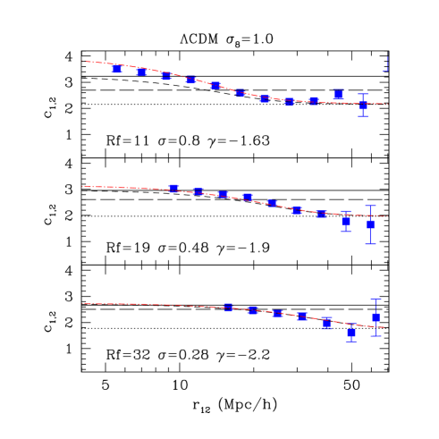
Figure 2: The hierarchical coefficient $c_{12}$ in the $\Lambda$CDM model as a function of the separation $r_{12}$. Each panel shows results for different smoothing scale $R_{f}$ as labeled in the Figure. Symbols show $c_{12}$ in the $\sigma_{8}=1.0$ output of the $\Lambda$CDM model, with errors corresponding to the variance in 5 realizations. The continuous line shows the leading order prediction for the skewness: $S_{3}\equiv c_{12}(r_{12}=0)=34/7+\gamma$. The long-dashed line corresponds to the PT result $c_{12}=68/21+\gamma/3$ (B96). The short-dashed line corresponds to the SC prediction, Eq.(43), which tends to $c_{12}=68/21+2\gamma/3$ (dotted-line) in the limit $\xi_{2}\rightarrow 0$. The dotted-dashed lines correspond to the 1-loop SC prediction, Eq.(34).

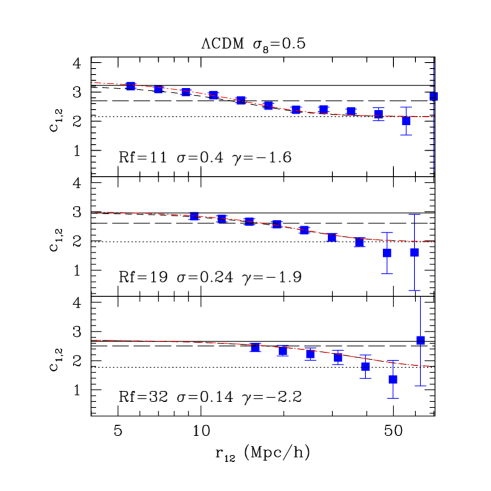
Figure 3: Same as Fig.2 for the $\sigma_{8}=0.5$ $\Lambda$CDM output.

4.3 The 2-point Skewness in the Weakly Non-linear Regime

Figures 2-3 show the 2-point skewness, $c_{12}\equiv{\cal K}_{12}/(\xi_{2}\sigma^{2})$, in the weakly non-linear regime, that is when the smoothing scale is such that the variance is small: $\sigma\la 1$. The figures show a comparison with $\Lambda$CDM simulations for a wide range of values of $\sigma=0.1-1.5$ ($\sigma^{2}=0.02-2$) corresponding to different scales, outputs and values of $\gamma$. The long-dashed line corresponds to the tree-level in PT prediction, Eq.(39). The short-dashed line corresponds to the leading order prediction for the 2-point skewness in the SC:

$$c_{12}=2~{}\overline{\nu_{2}}+\overline{\nu_{2}}~{}{\xi_{2}\over{\sigma^{2}}}={68\over 21}+{2\over 3}~{}\gamma+\left({34\over 21}+{\gamma\over 3}\right)~{}{\xi_{2}\over{\sigma^{2}}}$$ (43)

while the dotted lines gives the limit $\xi_{2}\rightarrow 0$, e.g, Eq.(40). The dot-dashed line includes the 1-loop SC correction (e.g, Eq.(34)). Each panel is labeled with the smoothing scale $R_{f}$ and the corresponding linear rms $\sigma(R_{f})$ and slope $\gamma$.

In all cases we see there is a very good agreement with the leading order SC prediction. Note that in the limit $\xi_{2}\rightarrow 0$ we recover the SC value in Eq.(43) (dotted line) rather than the rigorous PT prediction, Eq.(39) (long dashed line). This is a somewhat surprising result, as one would expect the rigorous PT prediction to be more accurate than the SC approximation. A possible explanation could be that the regime of validity of PT is out of the dynamical range proved in our simulations. However this is unlikely to be the case as we have managed to measure $c_{12}$ for scales as large as $R_{f}\ga 30{\,h^{-1}\,{\rm Mpc}}$ and $r_{12}\ga 50{\,h^{-1}\,{\rm Mpc}}$. On those scales the variance is $\sigma^{2}<0.02$ and $\xi_{2}$ approaches zero, where perturbative expansions of 2-point moments should yield accurate predictions.

On large scales the agreement with SC does not seem to depend on the value of the variance at the smoothing scale, except when we approach $\sigma\simeq 1$ and the perturbative approach itself breaks down (see §4.4).

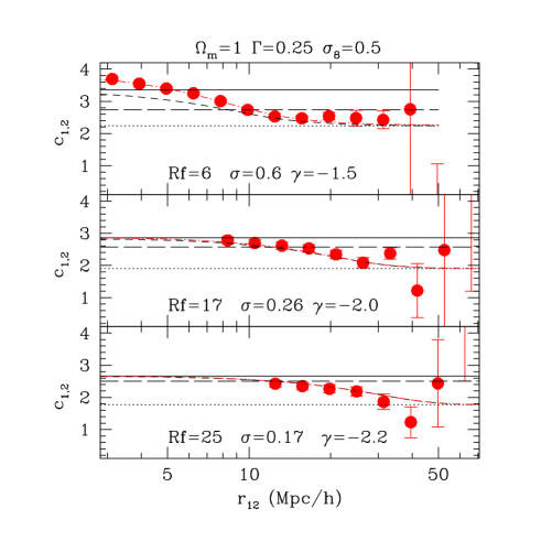
Figure 4: Same as Fig.2 for $\sigma_{8}=1.0$ $\Omega_{m}=1\times\Gamma=0.25$.

Fig.4 shows a comparison similar to Fig.3 for the $\Omega_{m}=1\times\Gamma=0.25$ model. The results are almost identical, indicating that they are insensitive to the value of $\Omega_{m}$ and to the particle resolution.

Fig. 5, shows the corresponding comparison for the realistic APM-like model. It displays large fluctuations at $r_{12}\simeq 50{\,h^{-1}\,{\rm Mpc}}$ which reflects the fact that the 2-point function in the APM-like model goes to zero on that scale. A similar problem arises around $r_{12}\simeq 40{\,h^{-1}\,{\rm Mpc}}$ for the SCDM model in Fig 6. As the two point function crosses zero quite sharply and the smoothing scale $R_{f}$ is large, the zero crossing affects a large range of scales $r_{12}\simeq 40{\,h^{-1}\,{\rm Mpc}}$ (typically a range $\pm R_{f}$).

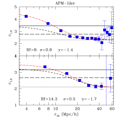
Figure 5: Same as Figure 2 for the APM-like model.

We can see Figure 5 that the SC prediction gives a much better match to the simulations than the PT predictions, in agreement with the cases discussed previously. Both in Fig 5 and 6 we can see how the SC model including the next-to-leading order (i.e, 1-loop correction) accurately reproduces the higher-order moments measured in simulations .

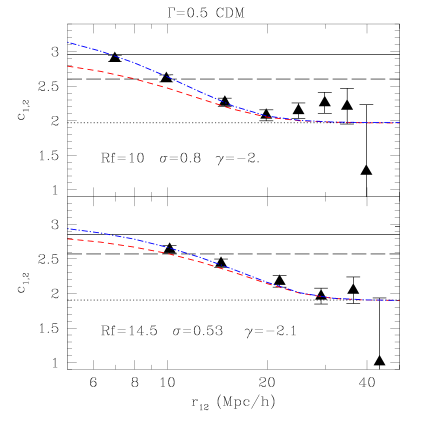
Figure 6: Same as Figure 2 for the $\Gamma=0.5$ CDM model.

4.4 The 2-point Skewness in the Non-linear Regime

Figure 7 shows a comparison for smaller smoothing radius. Here the variance at the smoothing scale $R_{f}\simeq 3-4$ is $\sigma^{2}\simeq 2$. Notice that, as expected, significant departures from the tree-level prediction in the SC model are observed on such small scales, i.e, when the variance largely exceeds unity. This is in agreement to what is already known for the skewness $S_{3}$. On the other hand, as can be seen in Fig 7, the SC predictions work well on large scales, where $\xi_{2}<1$ (e.g, for $r_{12}>8{\,h^{-1}\,{\rm Mpc}}$), even when $\sigma^{2}>1$. This is similar to what we found for $\xi_{2}$ in §4.2, which follows well linear theory even when the smoothing scale is fully non-linear.

For small smoothing radius $R_{f}$ the errors become much smaller and the SC gives a perfect match to Nbody measurements at large $r_{12}$. This says that the SC reproduces well the non-linear transition between small and large scales found in numerical simulations.

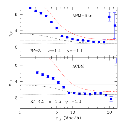
Figure 7: Same as Figure 2, but for smaller smoothing scales (which means larger values of the variance). The top (bottom) panel shows the APM-like ($\Gamma=0.2$ CDM) model.

In general, for $\sigma\la 0.8$ the results agree quite well with the perturbative SC model. In some cases, when $\gamma$ is large (flat slope) and $\sigma\simeq 1$ the amplitudes $c_{12}$ tend to increase at all scales, including at large $r_{12}$. This behavior is qualitatively predicted by the perturbative SC expressions as given by Eq.(34), although in the non-linear regime, there is no reason to expect that the term $\sim\sigma^{2}$ intrinsic to loop corrections in PT can accurately account for the gravitational evolution of the moments. We stress that the value of $\sigma$, where deviations from SC prediction take place, depends on the value of the smoothing parameter, $\gamma$, in agreement with the general trend found in FG98 for the 1-point moments: the larger the smoothing correction (or the smaller $\gamma$), the smaller the non-linear contribution to the moments (see Table 2 in FG98). This can also be seen at large scales ($r_{12}\ga 8{\,h^{-1}\,{\rm Mpc}}$) by comparing the two panels in Fig.7.

4.5 The 2-point Kurtosis

The analysis presented for the 2-point skewness above, can be straightforwardly extended to higher-order moments of the density field. In particular, we shall compare the results in the SC model for the 2-point estimators of the volume averaged 4-point function, what we shall call the 2-point kurtosis, Eqs.(35)-(36), with numerical simulations. This will allow us to assess how general are the results found from the analysis of the skewness. Figure 8 & 9 compare the SC prediction for the normalized 2-point kurtosis, $c_{13}$ and $c_{22}$, with the APM-like and CDM simulations, respectively. Note how the limit for large scales (dotted lines) is quite different for $c_{13}\rightarrow 6\nu_{2}^{2}+3\nu_{3}$ than for $c_{22}\rightarrow 4\nu_{2}^{2}$. In both cases the SC predictions are in agreement with simulations.

In general, for weakly non-linear scales, $\sigma\la 0.5$, the results agree quite well with the perturbative SC model. For larger values of $\sigma$ the amplitudes tend to increase at all scales, including at large $r_{12}$.

The observed behavior is qualitatively predicted by the perturbative SC model, Eqs.(35)-(36), although noticeable differences appear when $\sigma\ga 0.5$. This is due to the fact that the perturbative regime has a narrower domain of validity as one considers higher-order moments of the density field. This is so because loop corrections are relatively more important for the 2-point kurtosis (see the difference between short-dashed and dot-dashed lines in Figs 8 & 9) than for the 2-point skewness (see same lines in lower panels of Figs 5 & 6).

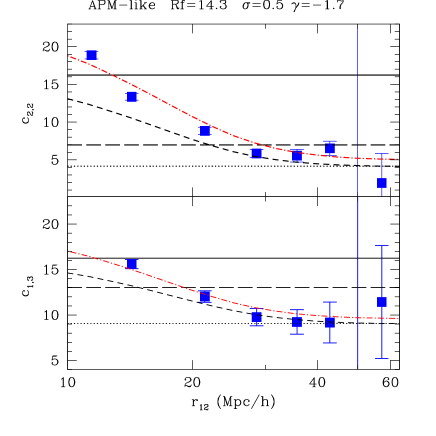
Figure 8: The hierarchical coefficients $c_{22}$ (top panel) and $c_{13}$ (bottom panel) in the APM-like model smoothed over a cell of $R_{f}=14.3$ ($\sigma=0.5$) as a function of the cell separation $r_{12}$. The continuous line shows the leading order prediction for the kurtosis: $S_{4}\equiv c_{13}(r_{12}=0)\equiv c_{22}(r_{12}=0)$. The long dashed line corresponds to the rigorous PT prediction. The short-dashed line corresponds to the SC leading order predictions, which tend to the dotted-lines in the limit $\xi_{2}\rightarrow 0$. The dotted-dashed line corresponds to the 1-loop SC prediction as given by Eqs.(35)-(36).

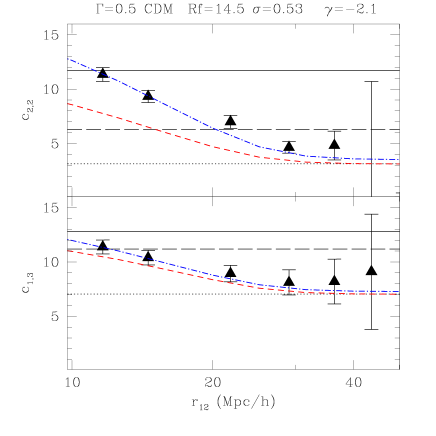
Figure 9: Same as Fig. 8 for $\Gamma=0.5$ CDM.

5 Conclusions

We have presented perturbative results for the 2-point moments of the dark matter density field within the SC model. In particular, we have derived expressions for the 2-point skewness and kurtosis in the weakly non-linear regime (see §3).

We have found an excellent agreement between the SC model and CDM and APM-like simulations at all relevant scales. When the variance $\sigma^{2}\la 0.5$ the perturbative SC model is in full agreement (within the error-bars) with measurements of the 2-point skewness and kurtosis from numerical simulations. When normalized to the second order statistics, we have confirmed that our results are insensitive to the cosmological parameters or to the amplitude of the initial fluctuations. We have tested the robustness of our findings against particle resolution and volume effects.

However, we have observed that the domain of validity of the perturbative SC model gets narrower as one considers higher-order moments of the density field, as seem in the analysis of the 2-point kurtosis (as compared to that of the skewness).

For larger values of the variance of the matter density field, $\sigma^{2}$, the perturbative approach is observed to break down, as expected. This is more extreme for smaller smoothing corrections. As we approach the strongly non-linear regime, $\sigma^{2}\ga 2$, the leading order SC predictions match the simulations quite well on scales $r_{12}>R_{f}$, while for $r_{12}\la R_{f}$ there are important non-linear effects which cannot not accounted for within our perturbative approach, as one would expect.

Our numerical simulations fail to match the leading order analytic predictions from perturbation theory (PT), derived by Bernardeau (1996, B96). In the unsmoothed case, these calculations are identical to the SC results presented here. But B96 found a different result for smoothed fields (ie compare Eq.[39] with Eq.[40]). Our failure to reconcile the simulations with the B96 predictions is puzzling. We have managed to extend our analysis to quite small values of the variance, i.e, $\sigma^{2}\la 0.02$, and we have considered large simulation boxes (up to $600{\,h^{-1}\,{\rm Mpc}}$) and also different resolution cells. It is unlikely that larger (realistic) simulations could resolve this problem as we are already probing scales where the two point function goes to zero and starts oscilating. On these larger scales, both simulations and predictions become uncertain. The deviations we find are quite significant, given the errors. One possible future approach could be to reduce the errors so as to be able to compare the predictions to earlier simulation outputs. This would allow us to explore the regime where $\sigma^{2}\la 0.02$, while $\xi_{2}$ is still positive.

The idea that PT could fail for $\sigma^{2}\simeq 0.02$ and start working for $\sigma^{2}\la 0.02$ is possible, but unlikely. Experience with other PT calculations and comparison with simulartions (e.g., with the bispectrum, see Scocimarro etal 1998) indicates good convergence even for relatively large variance $\sigma^{2}\ga 0.1$. It is reassuring that the perturbative SC approach works so well for a wide range of (realistic) situations, such as those we have explored here, so that in practice we should use these predictions (rather than B96) to compare to observations (see paper II). Note that the proposal by Szapudi (1998) to determine the bias with cumulant correlators will not work in the regime we are exploring here (unlike B96 predictions, the 1-point and 2-point SC predictions have the same smoothing corrections).

The 2-point moments should provide a convenient tool to study the statistical properties of gravitational clustering for fairly non-linear scales and complicated survey geometries, as those probing the clustering of the Ly$\alpha$ forest. In this context, the perturbative SC predictions presented here provide a simple and novel way to test the gravitational instability paradigm over a wide dynamical range.

References

- [1]
- [Baugh, Gaztañaga & Efstathiou 1995] Baugh, C.M., & Gaztañaga, E., Efstathiou, G., 1995, MNRAS, 274, 1049
- [Baugh & Gaztañaga 1996] Baugh, C.M., & Gaztañaga, E., 1996, MNRAS, 280, 37
- [Bernardeau 1992] Bernardeau, F., 1992, ApJ, 392, 1
- [Bernardeau 1994] Bernardeau, F., 1994, ApJ, 427, 51
- [Bernardeau 1996] Bernardeau, F., 1996, A&A, 312, 11 (B96)
- [Davis & Peebles, 1977] Davis, M. & Peebles, P.J.E., 1977 ApJS, 34, 425
- [Fosalba & Gaztañaga 1998] Fosalba, P., Gaztañaga, E., 1998, MNRAS, 301, 503
- [Fry 1984] Fry, J. 1984, ApJ, 277, L5
- [Gaztañaga & Croft 1999] Gaztañaga, E., Croft, R.A.C, 1999, MNRAS, 309, 885
- [Gaztañaga & Fosalba 1998] Gaztañaga, E., Fosalba, P., 1998 MNRAS, 301, 524
- [Gaztañaga & Yokoyama] Gaztañaga, E., Yokoyama, J., ApJ, 1993, 403, 450
- [Gaztañaga & Scherrer 2001] Gaztañaga, E., Scherrer, R.J, 2001, astro-ph/0105534, MNRAS, in press
- [Gaztañaga et al.] Gaztañaga, E., et al. , 2001, in preparation
- [Juszkiewicz et al. 1993] Juszkiewicz, R., Bouchet, F.R., & Colombi, S., 1993, ApJ, 412, L9
- [Peebles 1980] Peebles, P.J.E., 1980, The Large–Scale Structure of the Universe, Princeton University Press, Princeton (LSS)
- [Peebles 1993] Peebles, P.J.E., 1993), Principles of Physical Cosmology, Princeton University Press, Princeton
- [Scoccimarro & Frieman 1996a] Scoccimarro, R., & Frieman, J., 1996, ApJS., 105, 37
- [Scoccimarro & Frieman 1996b] Scoccimarro, R., & Frieman, J., 1996, ApJ, 473, 620
- [Scoccimarro 1998] Scoccimarro, R., 1998, MNRAS, 299, 1097
- [Scoccimarro 1998] Scoccimarro, R., Colombi, S., Fry, J. N., Frieman, J. A., Hivon, E., & Melott, A. 1998, ApJ, 496, 586
- [Szapudi(1998)] Szapudi, I. 1998, MNRAS, 300, L35