Clumpy outer Galaxy molecular clouds and the steepening of the IMF

We report the results of high-resolution ($\sim$0.2 pc) CO(1–0) and CS(2–1) observations of the central regions of three star-forming molecular clouds in the far-outer Galaxy ($\sim$16 kpc from the Galactic Center): WB89 85 (Sh 2-127), WB89 380, and WB89 437. We used the BIMA array in combination with IRAM 30-m and NRAO 12-m observations. The GMC’s in which the regions are embedded were studied by means of KOSMA 3-m CO(2–1) observations (here we also observed WB89 399). We compare the BIMA maps with optical, radio, and near-infrared observations. Using a clumpfind routine, structures found in the CO and CS emission are subdivided in clumps, the properties of which are analyzed and compared with newly derived results of previously published single-dish measurements of local clouds (OrionB South and Rosette). We find that the slopes of the clump mass distributions (–1.28 and –1.49, for WB89 85 and WB89 380, respectively) are somewhat less steep than found for most local clouds, but similar to those of clouds which have been analyzed with the same clumpfind program. We investigate the clump stability by using the virial theorem, including all possible contributions (gravity, turbulence, magnetic fields, and pressure due to the interclump gas). It appears that under reasonable assumptions a combination of these forces would render most clumps stable. Comparing only gravity and turbulence, we find that in the far-outer Galaxy clouds, these forces are in equilibium (virial parameter $\alpha\approx 1$) for clumps down to the lowest masses found (a few M_⊙). For clumps in the local clouds $\alpha\approx 1$ only for clumps with masses larger than a few tens of M_⊙. Thus it appears that in these outer Galaxy clumps gravity is the dominant force down to a much lower mass than in local clouds, implying that gravitational collapse and star formation may occur more readily even in the smallest clumps. Although there are some caveats, due to the inhomogeneity of the data used, this might explain the apparently steeper IMF found in the outer Galaxy.

1 Introduction

Studies of molecular clouds have spanned size scales from many tens to tenths of parsecs. The large-scale properties of molecular clouds can be studied throughout the Galaxy as well as in external galaxies. For the smallest structures in molecular clouds, however, lack of resolving power has limited detailed studies to molecular clouds nearest to the Sun. Therefore, it has never been investigated whether the effects of a different physical environment influences the properties of those structures. The possibility of making high-resolution maps with mm-interferometers allows a study of clump properties in clouds at much larger distances from the Sun, and therefore in a potentially different physical and chemical environment. The outer part of the galactic disk is such a region, where molecular clouds are more sparsely distributed (Wouterloot et al. wbbk (1990)), the diffuse galactic interstellar radiation field is weaker (Cox & Mezger cox (1989), Bloemen bloemen (1985)), the metallicity is lower (Shaver et al. shaver (1983), Fich & Silkey fichsilk (1991), Wilson & Matteucci wilson (1992), Rudolph et al. rudolph97 (1997)), and the cosmic-ray flux density is smaller (Bloemen et al. bloemenben (1984)), compared to the solar neighbourhood.

Previously, we have studied molecular clouds at galactocentric distances $R>$15 kpc (Brand & Wouterloot brandw1 (1994)) and analyzed molecular cloud properties across the Galaxy (Brand & Wouterloot brandw2 (1995), hereafter BW95). It was found that cloud kinetic temperatures as well as CO luminosities are similar to GMCs of the same mass in the solar neighbourhood. These results were in contradiction with those of Mead & Kutner (mead1 (1988)), who derived kinetic temperatures of 7 K for a sample of clouds at $R\sim$13 kpc, significantly colder than GMCs in the solar neighbourhood, and Digel et al. (digel (1990)), who found that outer Galaxy molecular clouds appear to be underluminous in CO with respect to their virial mass, by a factor of four, compared to local clouds (suggesting that the CO-to-H₂ conversion factor, $X$, should be four times higher). BW95 showed that the Digel et al. result is a consequence of the small number of clouds studied by them. BW95 also found that outer Galaxy clouds are generally less massive than inner Galaxy clouds, and that in the inner Galaxy there are relatively more large clouds (see also May et al. may (1997)); they furthermore noted that outer Galaxy clouds have larger radii than inner Galaxy clouds of the same mass, which in part could be explained by a lower pressure of the surrounding ISM at large $R$, allowing the clouds to settle at larger equilibrium radii. Wouterloot et al. (wouterfieg (1995)), and Fich & Terebey (fichter (1993)), using far-infrared luminosities of IRAS point sources in the outer Galaxy determined by Wouterloot & Brand (wb89 (1989); hereafter WB89), measured a slope for the initial mass function in the outer Galaxy that is steeper than the IMF measured in the solar neighbourhood. A similar indication of steepening has been found by Garmany et al. (garmany (1982)) from O-stars (M$>$20 M_⊙) within 2.5 kpc from the Sun. These differences are generally attributed to the different conditions in the outer Galaxy. On the other hand Casassus et al. (casassus (2000)), from a study of IRAS sources with the colours of UCHii regions concluded that the exponent of the IMF does not seem to vary.

The aim of the present study is to investigate the properties of molecular clumps (sizes from $0.2-2$ pc) in GMCs in the outer Galaxy, and to explain any differences with clump properties in local clouds in terms of effects due to a different physical environment. At the typical distances for these objects of 10 kpc, the resolution required for such a study is $\sim$ 5″, which can only be obtained by using an interferometer. We employed the BIMA mm-interferometer (Welch et al. welch (1996)) to map CO(1–0) and CS(2–1) in three molecular clouds at $R>$15 kpc. To compensate for the lack of zero-spacing information, which is particularly important for structures that are extended over size-scales larger than 1′, the data were complemented with observations from the Kitt Peak 12-m (CO) and the IRAM 30-m telescopes (CS). The combined maps allow us to compare clump properties in the far outer Galaxy with those obtained from single dish observations of nearby GMCs. Three clouds (2 of which were also observed with BIMA) were mapped with KOSMA, to allow derivation of their masses.

Sect. 2 describes the sample of objects, the observations and the data reduction. In Sect. 3 we present the results for the individual sources, while in Sect. 4 we describe the method used to identify clumps from the data. Sect. 5 is devoted to a discussion of the clump physical properties and a comparison with local clouds. In particular, in Sect. 5.1.4 we look at the implications of our observational results on the slope of the IMF as a function of $R$. In Sect. 6 we summarize the main results.

Table 1: BIMA observational parameters.

Source	IRAS	$\alpha$(1950)	$\delta$(1950)	Molecule	Array	beam	pixel	rms	K/Jy
WB89		h m s	° ′ ″			″	″	Jy
85	21270+5423	21 27 05.9	+54 23 42	CO(1–0)	B,C	10.7$\times$8.5	2	1.2	1.02
380	01045+6505	01 04 35.7	+65 05 21	CO(1–0)	B,C	7.2$\times$4.7	1.5	1.2	2.73
				CS(2–1)	B,C	8.9$\times$6.6	2	0.46	2.19
437	02395+6244	02 39 30.6	+62 44 22	CO(1–0)	C	21.8$\times$14.9	3	1.9	0.28
				CS(2–1)	C	19.3$\times$16.0	3	0.65	0.41

2 Observations and Data Reduction

2.1 Source Selection

The WB89-catalogue presents an extensive CO survey towards IRAS point sources located in the outer Galaxy (second and third quadrants), with infrared colours that discriminate in favour of sources frequently associated with H₂O masers and dense molecular cloud cores (Wouterloot & Walmsley wouterwalms (1986)), and hence with star forming regions. We selected the four sources at $R>$15 kpc with the highest far-IR luminosity, to wit WB89~85 (IRAS~21270+5423), WB89~380 (IRAS~01045+6505), WB89~399 (IRAS~01420+6401), and WB89~437 (IRAS~02395+6244). Unless specified otherwise, in the following we shall for convenience use the WB89-name to indicate the molecular clouds associated with these IRAS sources, rather than the IRAS source itself.

2.2 Single-Dish Observations

NRAO 12-m

WB89 85, 380, and 437 were observed using position switching on a 9$\times$9 grid with 30″ spacing in CO J=1–0 with the Kitt Peak 12-m telescope on December 4-9, 1991. The emission was found to extend beyond this region in all three cases; subsequently the GMC near WB89 85 was completely mapped. The telescope beamwidth at 115 GHz is 56″. The standard chopper wheel method (Ulich & Haas ulich (1976), Kutner & Ulich kutnerul (1981)) was used for calibration. All intensities are on a a $T_{\rm R}^{*}$-scale. System temperatures were typically 350 – 500 K. We used filterbanks of 128 channels of 100 kHz for each of the polarizations. The velocity coverage is therefore 33 kms^-1 with 0.26 kms^-1 resolution. After averaging, the rms noise level is $0.13-0.25$ K.

We have also observed ¹²CO(2–1), ¹³CO(1–0), CS(2–1), HCO⁺(1–0), and HCN(1–0) at various locations on and near the three main CO peaks surrounding IRAS21270+5423.

IRAM 30-m

WB89 85, WB89 380, and WB89 437 were observed in CS J=2–1, 3–2, and 5–4 with the IRAM 30-m telescope at Pico Veleta from July 24 – 26 1991. The maps are on a 11$\times$11 grid with 15″ spacing, covering all CS emission. The telescope beamwidth at these frequencies (98, 147, and 245 GHz) is respectively 26″, 16″, and 11″. The standard chopper wheel method was employed for temperature calibration. All intensities are on a $T_{\rm A}^{*}$-scale. System temperatures were typically 200 – 250 K. Using a 128 channel filterbank of 100 kHz per channel, the velocity coverage is 40 kms^-1 and the resolution 0.3 kms^-1. Observations were made by position switching; the typical rms noise level in the spectra is 0.08 K. Low-order polynomial baselines were subtracted. In addition, 15 more outer Galaxy clouds were observed in the same transitions, to search for potentially interesting objects. With a few exceptions, these were all single-pointed observations at the IRAS PSC position.

KOSMA 3-m

WB89 380, WB89 399, and WB89 437 were observed in ¹²CO(2–1) in August 1998 and September 1999 with the refurbished KOSMA 3-m telescope (see Kramer et al. 1998a ). The beamsize at 230 GHz is about 1$\aas@@fstack{\prime}$9 and the clouds were observed in position switching mode on a 1′ raster in galactic coordinates, covering the region where Brand & Wouterloot (brandw1 (1994)) detected ¹²CO(1–0) at the lower resolution (and raster) of about 4′. We used an acousto-optical spectrometer with a channel spacing of 167 kHz and effective resolution of 360 kHz (0.47 kms^-1). The sky transmission was estimated by measuring the radiation temperature of the blank sky at the elevation of the sources. Analogous to the standard chopper wheel calibration, the intensities were corrected to the $T_{\rm A}^{*}$-scale. The rms noise level in the spectra is about 0.10 – 0.15 K. For the mass calculations (see Sect. 3) we used $T_{\rm mb}$ ($\eta_{\rm mb}=0.7$).

2.3 Interferometer Observations

WB89 85, 380, and 437 were observed with the three-element BIMA interferometer in 1991 October, May and June, respectively. CO(1–0) observations of WB89 85 and WB89 380 were made with the B- and C-array, and of WB89 437 with the C-array. CS(2–1) observations of WB89 380 were made with the B- and C-array, and of WB89 437 with the C-array. Flux- and phase calibrators were 3C84, BL Lac, and 3C454. The primary beam of the array is 100″ at 115 GHz and 117″ at 98 GHz. Table 1 lists the parameters of the observations. The instrumental phase and gain were determined with the standard BIMA data reduction package Miriad.

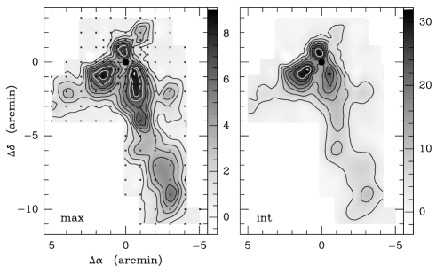
Figure 1: NRAO 12-m map of CO peak $T_{\rm R}^{*}$ (left) and $\int T_{\rm R}^{*}{\rm d}v$ (right) for $-100<V_{\rm lsr}<-88$ km s^-1 for WB89 85. Contour values are 1(1)9 K (left) and 4(4)32 Kkm s^-1 (right). The IRAS source position is indicated with the filled circle at (0,0), while the small crosses indicate the observed positions.

2.4 Combining Single-Dish and Interferometer Data

In all three sources the distributions of CO and CS are extended with respect to the BIMA synthesized beams, which implies that the interferometer observations are not sensitive to a significant fraction of the emission, due to a lack of information on the low spatial frequencies. This information has been obtained using the single-dish observations. The maps from the 12-m sample spatial frequencies from 0 to 4.5 k$\lambda$ in the uv-plane, and those from the 30-m sample spatial frequencies from 0 to 9.6 k$\lambda$.

The method used for this data combination is similar to that described by Vogel et al. (vogel (1984)) and Bieging et al. (bieging (1991)). A single dish observation is a convolution of the true spatial distribution of the emission with the beam. To take out the effect of this convolution, the maps were deconvolved using the CLEAN-algorithm. Similarly, an interferometer observation is a convolution of the true distribution of the emission with the primary beam of each of the BIMA telescopes. The deconvolved single-dish maps were convolved with the primary-beam pattern of the BIMA telescopes. To ensure correct scaling and positioning of the single-dish data with respect to the interferometer observations, maps were constructed from the interferometer and single dish uv-data separately covering only the overlapping part in uv-space. For the 12-m and BIMA comparison this involved a uv-range of 2.3 to 4.0 k$\lambda$, and for the 30-m and BIMA comparison we used 2.0 to 7.0 k$\lambda$. In these maps we found small offsets in the absolute positions between the single dish and the interferometer map centers. These were 10″ or less for the comparison with the 12-m maps, and 6″ or less for the 30-m maps. Since the pointing accuracy of the single-dish telescopes is worse than that of the interferometer, we corrected the central coordinates of the single dish maps to match those of the interferometer observations. The shifted maps made from the same limited uv-range were then used to derive the relative scaling of 35 Jy/K for the 12-m CO observations, and 9 Jy/K for the 30-m CS(2–1) observations. These values are within 5% of the theoretical gain of the single-dish antennas.

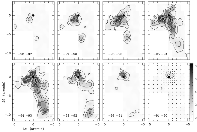
Figure 2: NRAO 12-m ¹²CO(1–0) map of the WB89 85 cloud, showing channel maps in 1 kms^-1 intervals. Contour values are 0.5(1)8.5 Kkms^-1. Symbols as in Fig. 1

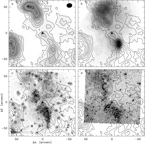
Figure 3: a High-resolution BIMA CO image of the WB89 85 region. The emission is integrated over $-98.25<V_{\rm lsr}<-89.50$ km s^-1, and the (primary beam-corrected) contour levels are 14(14) Kkms^-1. The resolution of the BIMA synthesized beam is indicated in the upper righthand corner. The filled circle is the IRAS source, the thick dotted contour is the associated error ellipse. b The BIMA CO contours superimposed on the distribution of the 6-cm continuum radiation (halftone and dotted contours), with a peak flux in the map of about 170 mJy/beam. c As b, but with the BIMA CO contours superimposed on the optical image from the DSS. For clarity, the more intense optical emission has been contoured (white). d As c, but with the BIMA CO contours superimposed on the K-frame obtained by de Geus & E. Lada (pers. comm.). The cuts of the gray scale have been set to show the low-level emission; for clarity, the more intense K-emission has been contoured (white; the lower levels only, to avoid confusion).

After applying the shift and gain, the single-dish maps were (fast) Fourier-transformed to uv-space and sampled on a set of eight circular tracks in the uv-plane from 0 to 4.0 k$\lambda$ for the 12-m maps and from 0 to 8.0 k$\lambda$ for the 30-m maps. To check this procedure, the uv-datasets acquired in this way were Fourier transformed back into map space; the resulting maps as well as the beam profiles were compared to the input maps and beam patterns. The maxima and the total fluxes of the maps agree to with 3%, and Gaussian fits to the beam maps give beam profiles that are within 2% of the nominal sizes of the single-dish beams.

The single-dish uv-data were then combined with the uv-datasets from the interferometer. Complete data cubes were subsequently obtained by Fourier transforming the combined uv-datasets to the map plane, using the Miriad routine INVERT, with natural weighting (which is essential to maintain the appropriate relative weights of the single-dish and interferometer contributions). From the resulting cubes the “dirty” beam was deconvolved using the Miriad routine CLEAN, and convolved with a “clean”-beam using RESTORE. From the separate planes in the data cubes the CLEAN and RESTORE procedure left only the inner quarter with useful data, which was extracted from the cubes. In order to correct for the response of the primary beam of the interferometer elements, these data cubes were divided by the normalized primary beam profile. This final procedure allows us to determine clump properties confidently over the whole image, but has the important disadvantage that the noise is not uniform over the image. This leads to uncertainties in the clump finding process, which will reflect on the completeness of the clump search, particularly for the weakest (i.e. smallest and least massive) clumps.

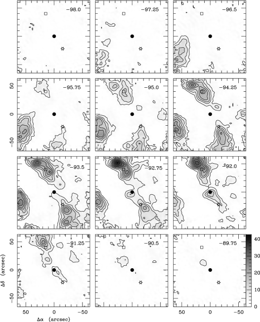
Figure 4: High-resolution ¹²CO(1–0) channel maps of the Sh 2-127 region showing the velocity structure between –98.0 and –89.75 km s^-1. Each panel shows the emission in a 0.75 kms^-1 wide interval, centered at the indicated velocity. The position of the IRAS source WB89 85 is indicated by the filled circle and that of the compact Hii region/radio component B by the asterisk. The square denotes the position of the peak of radio component A (see text). Contour levels are 4(4) Kkms^-1.

3 Results

WB89 85 (IRAS 21270+5423) is located in Sh~2-127, which is an optical Hii region at a kinematic distance of 15.0 kpc from the galactic center and 11.5 kpc from the Sun. The associated molecular cloud was completely mapped in CO with the NRAO 12-m at Kitt Peak. Fig. 1 shows the NRAO 12-m CO map of peak temperature (left) and integrated emission (right). From the total CO luminosity, and using a value for the $X$-factor ($N{\rm(H_{2})}/W_{\rm CO}$) of 1.9$\times$10²⁰ (Strong & Mattox strongmat (1996)), we derive a mass $M_{\rm CO}$ (see Sect. 4) for this molecular cloud of 1.6$\times 10^{4}$ M_⊙. The IRAS far infrared luminosity of the point source is $L_{\rm fir}$=1.0$\times 10^{5}$ L_⊙, which indicates the presence of the equivalent of an O7 V₀ star (or O8-8.5 V; Panagia panagia (1973)). The relevant parameters of this cloud, and the other clouds, are collected in Table 2. Fig. 1 shows that the IRAS source is located in a relative minimum, and is surrounded by three main clouds. From the channel maps in Fig. 2 we see that most of the emission is between $-$95 and $-$93 kms^-1, and that the three clouds near the IRAS source all have the peak of their emission at different velocities.

Table 2: Cloud parameters.

Source	$d$	$R$	$L_{\rm fir}$	$M_{\rm CO}$	$r_{\rm eff}^{\clubsuit}$
WB89	(kpc)	(kpc)	(104 L⊙)	(104 M⊙)	(pc)
85	11.5	15.0	10	1.61	11.41
380	10.3	16.6	10	3.52	22.42
399	9.9	16.6	4.3	2.62	21.32
437	9.1	16.2	7.1	0.942	13.32
♣ Effective radius, $r_{\rm eff}=\sqrt{Area/\pi}$, corrected for beam size
1 From NRAO 12-m CO(1–0) data
2 From KOSMA 3-m CO(2–1) data

Radio-continuum observations (Rudolph et al. rudolph (1996)), revealed the presence of an extended source (their component A; deconvolved size 30″), and a compact Hii region (their component B; deconvolved size 9″), about 1′ to the southwest. Both components are connected and enveloped by low-level diffuse emission (see Fig. 1 in Rudolph et al.), and indicate the presence of the equivalent of one O7 and one O8.5 V₀ star, for components A and B, respectively, consistent with the IRAS luminosity.

Fig. 3a shows the distribution of the integrated CO intensity towards Sh 2-127 obtained from the BIMA and the NRAO 12-m observations, corrected for the primary beam of the BIMA antennas. It shows the three main clouds from Fig. 1, as well as some low-intensity emission.

The distribution in velocity of the CO emission is shown in Fig. 4. The emission is quite structured, and several emission peaks can be seen in each panel; in Sect. 4 we use a clump finding program that leads to the identification of 62 clumps in these data.

Figure 5: Spectra at four positions towards WB89 85 extracted from the BIMA CO datacube, averaged over 5$\times$5 pixels of 2″ centered at the indicated offset from the map center.

The CO peaks in the interferometer map were searched for CS emission with the IRAM 30-m telescope. A CS core of size (at 1–2$\sigma$ level) $\approx$ 50″$\times$60″ (2.8 pc $\times$ 3.4 pc) was detected towards the northern CO peak, centered at offset $\sim$(17″,49″). This corresponds to within 5″ with both the position of the northern radio continuum peak and the northern CO-peak. A search with the NRAO 12-m for the higher-density tracing transitions CS(2–1) and HCN(1–0) towards the easternmost CO peak in the single-dish CO map has resulted in the detection of both molecules ($T_{\rm R}^{*}\sim 0.3$ K), which implies densities of at least a few times 10⁴ cm^-3 (e.g. Evans evans (1999)); likewise, HCO⁺(1–0) was searched for and detected ($T_{\rm R}^{*}\sim 0.5$ K) towards all three CO peaks that surround the IRAS position. A fit to the hyperfine lines in the HCN(1–0) sum-spectrum indicates that the emission is optically thin ($\tau\sim 0.6\pm 0.7$).

In Fig. 3b, c, and d we compare the integrated CO distribution with respectively the VLA 6-cm radio continuum map (Rudolph et al. rudolph (1996)), the optical image, taken from the Digital Sky Survey (DSS), and a 2 $\mu$m (K-band) image, obtained with the 4-m telescope at Kitt Peak, by de Geus & E. Lada (pers. comm.).

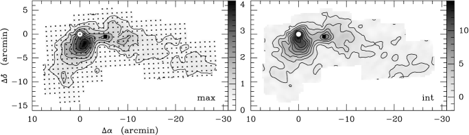
Figure 6: KOSMA ¹²CO(2–1) map of the cloud associated with WB89 380, showing the peak (left) and integrated CO intensity (right) from $-92<V_{\rm lsr}<-82$ km s^-1. The lowest contour level and contour step are 0.5 and 0.5K (left) and 1.0 and 1.5 K km s^-1 (right). Indicated are the locations of two IRAS point sources that were included in Wouterloot & Brand (wb89 (1989)): WB89 379 (IRAS 01037+6504; square) and WB89 380 (circle; at (0,0)). The small crosses indicate the observed positions. The interferometer observations are centered on the position of WB89 380.

The diffuse radio continuum emission covers much of the area in Fig. 3b, and correlates (together with the components A and B) fairly well with that of the high-resolution CO emission, although there are significant differences (see below).

The optical- and the CO emission are clearly anti-correlated. Comparison of Fig. 3b and c shows that the optical emission of component A is for the most part obscured by, and therefore located behind, the large northern CO complex: only some relatively faint emission of this component is optically visible, beyond the western edge of the obscuring molecular cloud, which shows that component A is not (completely) embedded. Its peak is slightly offset to the SW from the main CO peak, but coincides with a clump (nr. 10 in Table 3).

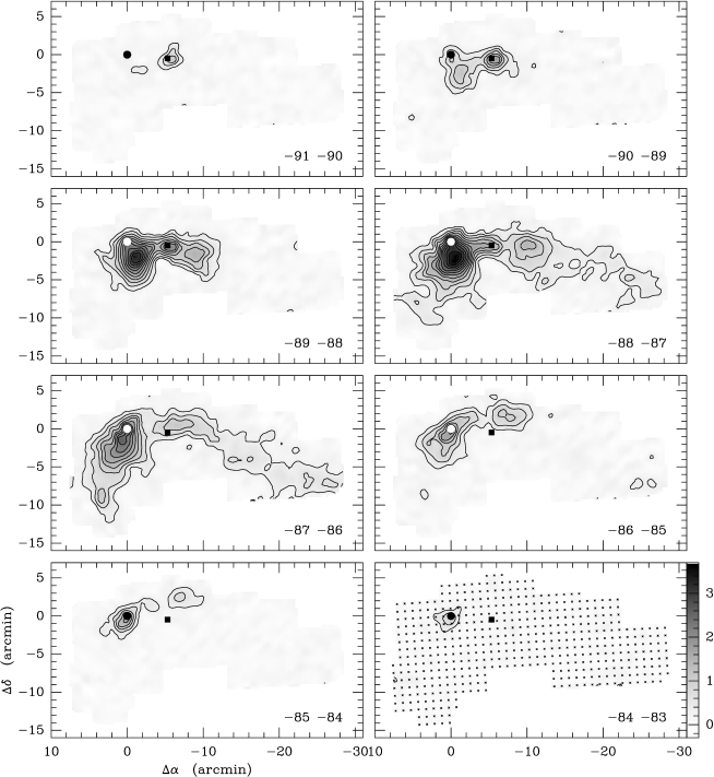
Figure 7: KOSMA ¹²CO(2–1) map of the WB89 380 cloud, showing channel maps in intervals of 1 km s^-1. The lowest contour level and contour step are 0.3 K km s^-1. Symbols are as in Fig. 6.

The optically visible compact Hii region (component B) lies at the eastern edge of a patch of obscuration (Fig. 3c), which corresponds to a peak in the CO emission, and the Hii region must therefore lie on the near side of the molecular complex. This is confirmed by the fact that Fich et al. (fichha (1990)) find $V_{\rm lsr}$(H_α) = $-98\pm 0.4$ kms^-1, which indicates that the ionized gas is moving towards us with respect to the molecular cloud. The radio peak B (Fig. 3b) is slightly displaced to the West with respect to the optical emission (Fig. 3c), which indicates that this region is still partially obscured. At the radio peak $\int T{\rm(CO)d}v\approx 41.3$ Kkms^-1, which translates into $N{\rm(H_{2})}\approx 7.8\times 10^{21}$ cm^-2, corresponding to a visual extinction $A_{\rm v}\approx$ 8 mag. Likewise, $\int T{\rm(CO)d}v$ seen projected on the optically visible part of the Hii region corresponds to $A_{\rm v}\approx$ 2 mag, and probably most of that CO lies behind the optically visible emission. The Hii region therefore lies in a cavity in the southwestern molecular cloud; the cavity is open towards the East, where we can see the ionized gas optically, while the wall of the cavity closest to us causes the rest of the Hii region to be obscured by about 6 mag. The compact Hii region is associated neither with a temperature peak in Fig. 4, nor with a peak in $\int T{\rm d}v$ in Fig. 3. It also does not lie near the center of any of the identified clumps. The clumps just to the SW and NE of the Hii region (resp. nrs. 11 and 14 in Table 3) are at different velocities (resp. –93.8 and –92.5 km s^-1). Because the ionized gas is breaking through the cloud, it has removed molecular gas from the line-of-sight. In Fig. 5 we show CO spectra towards four offset positions: that of the position of WB89 85 at (0″,0″), the compact Hii region to the SW ($-$16″,$-$22″), the CO peak near that ($-$20″,$-$30″), and the strong northern maximum (26″,50″).

A comparison of the K-band emission with the optical image shows there are about 40 objects that are visible in the NIR, but not on the DSS. Considering the distance of this object, and its location in the outer Galaxy, it’s unlikely that many, if any, of these K-band sources are reddened background stars. One of these objects lies at the position of the peak of radio component A, and might be its exciting source. These NIR data will be discussed in detail in a separate paper. The IRAS source is seen projected on top of a small clump. It is unclear whether there really is a YSO at this position or whether the PSC position results from confusion due to nearby sources north and south.

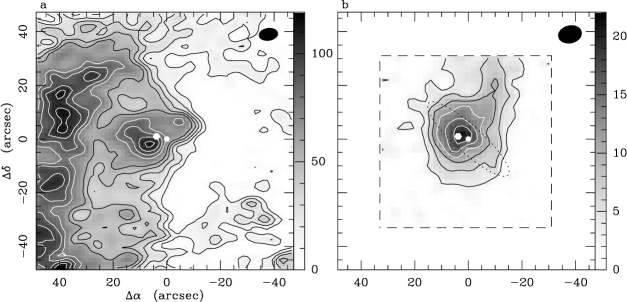
Figure 8: High-resolution images of the WB89 380 region. The position of the compact Hii region (point source at 6 cm), detected with the VLA is indicated by the hexagon. The IRAS source is shown as a filled circle. a The BIMA interferometer integrated ($-89.75\leq V_{\rm lsr}\leq-83.25$) CO map, with the contour levels: 11(11) Kkms^-1; b The integrated ($-90.55\leq V_{\rm lsr}\leq-83.35$) CS distribution, with the contour levels 3(3) Kkms^-1. The error ellipse of the IRAS source is shown as well. There are no data in this panel outside the dashed box.

WB89 380 (IRAS 01045+6505). There is no association with an optical Hii region for this object. WB89 reported two velocity components for this line of sight, of which the brighter one is at –88 km/s. More recent ¹³CO and C¹⁸O observations (Wouterloot & Brand wb96 (1996)) reveal that the ¹²CO(1–0) is self absorbed, however, and that the central velocity is actually –86 km/s. This leads to a kinematic galactocentric distance of 16.6 kpc and a heliocentric distance of 10.3 kpc. WB89 380 has a FIR luminosity of 1.0$\times$10⁵ L_⊙, which suggests the presence of an O7 V₀ star (or O8-8.5 V; Panagia panagia (1973)). This object was observed at the VLA at 6, 3.6 and 2-cm by Rudolph et al. (rudolph (1996)); a point source was detected at the IRAS PSC position. From the continuum data, a spectral type of O7.5 V₀ (O8.5 V; Rudolph et al. rudolph (1996)) is derived, which is consistent with that deduced from the FIR luminosity.

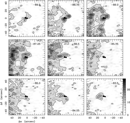
Figure 9: High-resolution ¹²CO(1–0) channel maps of the WB89 380 region showing the velocity structure between –89.5 and –83.5 km s^-1. Each panel shows the emission in a 0.75 kms^-1 wide interval, centered at the indicated velocity. Contour levels are 6(6) Kkms^-1. The filled circle indicates the position of WB89 380, the hexagon that of the compact radio source.

Fig. 6 shows the single dish ¹²CO(2–1) map obtained with the KOSMA 3-m telescope, from which we derive a mass $M_{\rm CO}=3.5\times 10^{4}$ M_⊙ ($X=1.9\times 10^{20}$, assuming a ratio (2–1)/(1–0) of 0.85 (BW95), and $\eta_{\rm mb}=0.7$), and a radius $r_{\rm eff}$ = 22.4 pc (see Table 2). In Fig. 6 there is a strong maximum towards WB89 380, and a weaker one towards WB89 379. Furthermore there is extended emission at a level of about $T_{\rm A}^{*}$=1 K with line widths less than 2 km s^-1. The channel maps in Fig. 7 show that most emission is at –88 to –86 km s^-1. Northwest of WB89 379 there is a separate component at about –86 km s^-1. Towards this IRAS source both components overlap (double lines are seen), while towards WB89 380 lines are much broader and profiles are asymmetric, and are affected by the self-absorption mentioned above. The highest temperatures occur south of this source.

The BIMA observations are centered on the IRAS point source WB89 380, located near the strongest CO peak of the cloud. Fig. 8a shows the BIMA integrated CO emission, and Fig. 8b shows the same for the CS integrated emission.

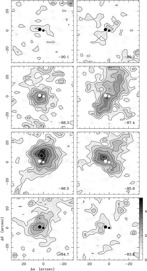
Figure 10: High-resolution CS(2–1) channel maps of the WB89 380 region showing the velocity structure between –90.1 and –83.8 km s^-1. Each panel shows the emission in a 0.9 kms^-1 wide interval, centered at the indicated velocity. Contour levels are 0.6(0.6) Kkms^-1. The filled circle indicates the position of WB89 380; the hexagon identifies the compact radio source.

Figure 11: Spectra at three positions towards WB89 380 extracted from the CO and CS datacubes, averaged over 5$\times$5 pixels of 1$\aas@@fstack{\prime\prime}$5 (CO) or 2″ (CS), centered at the indicated offsets from the map center. The absence of CO emission at the line center (i.e. the location of the CS emission peak) is due to self absorption.

The unresolved compact Hii region lies at the edge of a peak in the CO intensity map, but its position coincides almost exactly with the peak in the CS distribution, suggesting that the ionizing star(s) is (are) still embedded in the dense gas. This is confirmed by the detection of an H₂O maser towards WB89 380 (Wouterloot et al. wbf (1993); Comoretto et al. comore (1990)). The velocity structure of the CO and CS emission is shown in Figs. 9 and 10, respectively. There is an indication of a ring-like structure in the CO line at velocities between –89 and –87 km s^-1, perhaps caused by dynamical interaction of earlier formed stars with the gas.

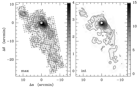
Figure 12: KOSMA ¹²CO(2–1) map of the cloud associated with WB89 399, showing the peak (left) and integrated CO intensity (right) from $-86<V_{\rm lsr}<-77$ km s^-1. The contour levels are 0.3 (0.3) 1.2 (0.6) 3.6 K(left) and 1(1) K km s^-1 (right). The circle at(0,0) indicates the location of the IRAS point source. The small crosses indicate the observed positions.

In the CS channel maps we note that while at the extreme velocities ($<-88$ and $>-85$ kms^-1) the emission peaks at the location of the compact radio source, it is offset from this position at the intermediate velocities, where it also has a larger extent. This behaviour is reminiscent of that of an expanding or contracting shell around the radio source, and deserves study at higher angular resolution.

We can use the present data to estimate the age of the Hii region. Assuming the structure we see in the CS channel maps in Fig. 10 is in fact an expanding shell, i.e. gas being swept up by the expanding Hii region, the expansion velocity of the shell $\approx 1.8$ kms^-1. The mass of the gas is $\sim$350 M_⊙, which is the average between the LTE mass of the gas (assuming $T_{\rm ex}=30$ K, and a [CS]/[H₂] abundance of 1.0$\times 10^{-8}$) and the sum of the virial masses of the clumps (see Table  5). Then the kinetic energy of the shell $E_{\rm kin}\approx 1.1\times 10^{46}$ erg. The central star is of type O7 V₀, has a luminosity of 10⁵ L_⊙, of which a fraction of 0.35 (Panagia panagia (1973)) is available in the Lyman continuum, i.e. $1.3\times 10^{38}$ ergs^-1. The efficiency with which this stellar energy is transformed into mechanical energy is about 0.1% (Spitzer spitzer (1978)). To arrive at the observed kinetic energy of the shell thus requires $\sim 3000$ yrs. The radius of the Hii region is 0.65 pc (Rudolph et al. rudolph (1996)). An Hii region around an O7 V₀ star reaches this radius after $\sim 1.2-3.8\times 10^{3}$ yrs (Spitzer spitzer (1978)), for initial densities of the embedding medium of $10^{7}-10^{8}$ cm^-3 (a reasonable estimate, see also De Pree et al. depree (1995)). This calculation is for the case of no absorption of the Lyman continuum photons by dust; with a fractional absorption by dust, it takes somewhat longer to reach a certain radius at the same initial density, but for the purpose of making a rough estimate the difference is negligible. This time interval is consistent with the 3000 yrs estimated above. In these considerations we have ignored the contribution of stellar wind to the energy budget: with a mass loss rate of $\sim 10^{-7.5}$ M_⊙yr^-1 and a wind velocity of $\sim 10^{3}$ kms^-1 (Garmany et al. garmetal (1981)) the available energy $\approx 2.4\times 10^{34}$ ergs^-1, four orders of magnitude less than the energy available in Lyman continuum photons.

Fig. 11 shows spectra for the CO and CS lines derived from the interferometer data, by summing all spectra in a box of 7$\aas@@fstack{\prime\prime}$5$\times$7$\aas@@fstack{\prime\prime}$5 (CO) or 10″$\times$10″ (CS) towards three offset positions. The CS spectrum peaks at –87 km/s, where the CO spectrum shows a dip, due to self-absorption. From these maps it is evident that the source is in an early stage of evolution with the young stellar object(s) still embedded in a high density clump. At 2 $\mu$m de Geus & E. Lada (pers. comm.) have found a cluster of stars centered on the CS clump. WB89 380 is therefore in an earlier stage of evolution than WB89 85, where alongside a young region (the northern CS core and possibly the NIR objects, if they are embedded) we also find more evolved objects.

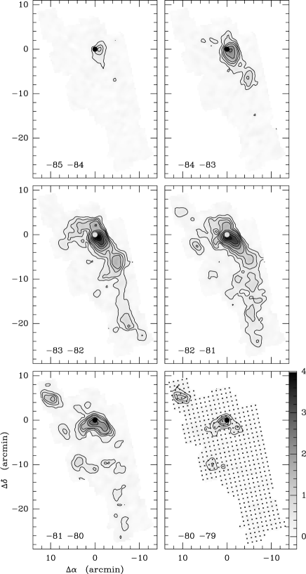
Figure 13: KOSMA ¹²CO(2–1) observations of WB89 399, showing channel maps in intervals of 1 km s^-1. The contour levels are 0.3 (0.3) 1.2 (0.6) 3.6 K km s^-1. Symbols are as in Fig. 12.

WB89 399 (IRAS 01420+6401). Towards WB89 399 an (optically visible) resolved Hii was detected with the VLA (see Rudolph et al. rudolph (1996)). The radio data suggest excitation by an O9.5 V₀ star, while the FIR luminosity of 4.3$\times 10^{4}$ L_⊙ implies a spectral type of O9-9.5 V₀ (or B0 V; Panagia panagia (1973)). The region was originally mapped in ¹²CO(1–0) and, incompletely, in ¹²CO(2–1) by Brand & Wouterloot (brandw1 (1994)). We present in Fig. 12 a new, complete ¹²CO(2–1) map of this region, made with KOSMA; due to lack of time, no BIMA observations were made. There is a strong maximum slightly southwest of WB89 399, located in a ridge of emission. In addition there are more isolated and weaker cloud components, in general with small line widths. Fig. 13 shows the velocity distribution. The strongest emission is at –83 to –81 km s^-1 with some weaker components at other velocities. The mass derived from the CO(2–1) data, assuming an intensity ratio of (2–1)/(1–0) of 0.85, $\eta_{\rm mb}=0.7$, and $X=1.9\times 10^{20}$, is $M_{\rm CO}=2.6\times 10^{4}$ M_⊙; the effective radius $r_{\rm eff}$ = 21.3 pc (see Table 2).

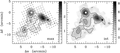
Figure 14: KOSMA ¹²CO(2–1) map of WB89 437, showing the peak (left) and integrated CO intensity (right) from $-80<V_{\rm lsr}<-68$ km s^-1. The lowest contour level and contour step are 0.5 and 0.5K (left) and 1.0 and 1.5 K km s^-1 (right). The triangles show the locations of two IRAS point sources that were included in Wouterloot & Brand (wb89 (1989)): WB89 436 (IRAS 02383+6241; square) and WB89 437 (circle). The small crosses indicate the observed positions. The interferometer observations are centered on the position of WB89 437.

WB89 437 (IRAS 02395+6244). This object has a FIR luminosity of 7.1$\times$10⁴ L_⊙, which indicates the presence of an O8 V₀ star (or O9-9.5 V; Panagia panagia (1973)). In the radio continuum observations, however, WB89 437 was not detected, putting an upper limit to the spectral type of a (single) embedded object of B1 (Rudolph et al. rudolph (1996)). These authors considered various scenarios to explain the discrepancy between the radio continuum and FIR observations, such as the presence of a very rich cluster of non-ionizing main-sequence stars of spectral type later than B1, large enough to produce the $L_{\rm fir}$ of 7.1$\times 10^{4}$ L_⊙, or the presence of a large amount of dust within the Hii region, that would have to absorb $\sim$90% of the UV radiation. Other possibilities are that an Hii region is present, but that it is very young and still optically thick. It is also possible that $L_{\rm fir}$ is generated by infall; a small amount of infalling matter would be enough to quench the forming of an Hii region around the embedded massive object (Molinari et al. molinari (1998); Walmsley walmsley (1995)).

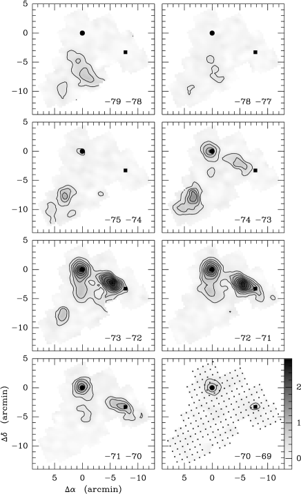
Figure 15: KOSMA ¹²CO(2–1) observations of WB89 437, showing channel maps in intervals of 1 km s^-1. The lowest contour level and contour step are 0.3 K km s^-1. Symbols are as in Fig. 14.

Fig. 14 shows the KOSMA ¹²CO(2–1) map of WB89 437. With the same assumptions as before, we derive a mass $M_{\rm CO}=9.4\times 10^{3}$ M_⊙, and a radius $r_{\rm eff}$ = 13.3 pc (see Table 2). There are two main clumps, near WB89 436 and 437 respectively, and several cloud components with weaker emission. The optically visible WB89 436 (see Rudolph et al. rudolph (1996)) is displaced from the center of the associated CO cloud, whereas WB89 437 is deeply embedded and shows strong outflow emission (Wouterloot & Brand wb96 (1996)). Channel maps of the ¹²CO(2–1) emission are shown in Fig. 15. The main clouds are at a velocity of $-73$ to $-71$ km s^-1, but the components in the southeastern part show emission at velocities down to –79 km s^-1.

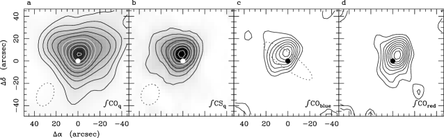
Figure 16: Results of the mm-interferometer measurements of WB89 437. The circle indicates the IRAS PSC position; the dotted ellipse in panels a and b represents the beam; the dotted contour in panel c is IRAS error ellipse. No primary-beam correction has been applied. a Integrated CO emission from $-$75 to $-$67.5 km s^-1. Lowest contour level and step are 17 Kkms^-1. The range of the grey scale is -10 (white) to 185 Kkms^-1 (black). b Image of integrated CS emission from from $-74$ to $-68.9$ km s^-1. Contour levels are 1.8 to 14.4 Kkms^-1 in steps of 1.8 Kkms^-1. The range of the greyscale is -1 (white) to 14 Kkms^-1 (black). c,d Contour plot of the CO emission, integrated over velocity intervals covering the blue (c) and red wing (d). The integration intervals are $-81<V_{\rm lsr}<-78\leavevmode\nobreak\$km s^-1 and $-66.5<V_{\rm lsr}<-63.5$ km s^-1. The contour levels are 1.4(1.4) Kkms^-1.

The BIMA observations were centered on the IRAS point source. Fig. 16a and b show the distribution of the integrated CO and CS emission, respectively. Unfortunately only C-array interferometer observations were obtained for this source in both CO and CS, which results in maps of relatively low resolution (18″=0.8 pc). Both CO and CS peak near the position of the IRAS point source, and the observations reveal a compact clump in both molecules. Near-IR observations of WB89 437 have led to the detection of an embedded young cluster centered on the dense core of the molecular gas (de Geus & E. Lada, pers. comm.). Fig. 16c and d show two velocity-integrated maps, covering the velocity ranges of the blue and red wings of the profile, respectively; the emission centers are offset by 6″. Spectra at the peak of the CO and CS emission at (0″,6″) are shown in Fig. 17. The presence of strong wing emission is evident from the CO spectrum, confirming the interpretation that the embedded cluster is producing outflowing gas. Unfortunately the available velocity range is too small to cover all outflow gas (cf. Fig. 17), and therefore we cannot derive the outflow parameters. The IRAM CS observations (not shown) also show this outflowing gas. The early evolutionary state of this source is also confirmed by the detection of an H₂O maser towards this source (Zuckerman & Lo zuck (1987); Wouterloot et al. wbf (1993)).

Figure 17: Spectra towards the peak of the integrated CO and CS emission of WB89 437, extracted from the BIMA datacubes, averaged over 5$\times$5 pixels of 3″ centered at the indicated offset (in arcsec) from the map center.

4 Clump Analysis

The observations have been analysed using the three-dimensional clump detection and analysis program CLUMPFIND described by Williams et al. (williams (1994)). The clump analysis has been carried out on both the CO and the CS data. Table 3 lists the properties of the CO clumps in WB89 85, the clump properties for WB89 380 are listed in Table 4 (from CO) and 5 (from CS), and Table 6 lists the clump properties for WB89 437 (both CO and CS). Note that the tables list only the resolved clumps, i.e. those for which an accurate value of the radius could be derived. Most of the clump parameters are self-explanatory, but a few require additional comments.

Col. 7 gives the effective radius $r_{\rm eff}$ of the clumps, which was derived from the measured effective radius at the lowest usable intensity level of the map (which we put at 2.5 $\sigma_{rms}$): $r_{\rm eff}=\sqrt{r_{\rm eff,obs}^{2}-r_{\rm beam}^{2}}$, where $r_{\rm beam}$ is the beam size. $r_{\rm eff,obs}=\sqrt{A/\pi}$ has been obtained by measuring the area ($A$) of the total extent of the clump when integrated over its full velocity range. At this low intensity level (relative to the clump maximum), the beam will have a size which differs from the usually reported full-width at half maximum (FWHM) beam size. Assuming the beam is Gaussian, the appropriate beam size can be calculated for each clump from the ratio of the peak temperature ($T_{\rm peak}$) of the clump to the actual temperature ($T$) at which the size is measured, and expressed in terms of the $FWHM$: $r_{\rm beam}=0.6\sqrt{\ln T_{\rm peak}-\ln T}\times FWHM_{\rm beam}$.

The FWHM linewidths of the clumps, $\Delta v$, are listed in column 8 and were calculated from the formal one-dimensional velocity dispersion $\sigma$ through $\Delta v^{2}$=8ln2 $\sigma^{2}$.

The CO luminosity, $L_{\rm CO}($K km s^-1 pc²) is calculated by adding the signals of all pixels that are assigned to a particular clump, and multiplying with the channel width in km s^-1 and the pixel area in pc². The mass of the clump is then determined from $M_{\rm CO}$/M_⊙=5.0 ($X$/2.3) $L_{\rm CO}$ (including a correction of 1.36 for He), where $X$ is the conversion factor from CO integrated intensity to molecular hydrogen column density (in units of $\rm 10^{20}(Kkms^{-1})^{-1}cm^{-2}$). We use $X$=1.9, the value derived by Strong & Mattox (strongmat (1996)); hence $M_{\rm CO}$/M_⊙=4.13 $L_{\rm CO}$ (Col. 9). The lowest, highest $M_{\rm CO}$ found are 3.3, 349 M_⊙ in WB89 85, 2.0, 62.4 M_⊙ in WB89 380, and 9.7, 480 M_⊙ in WB89 437. CLUMPFIND managed to allocate virtually all emission in the maps to clumps: 99.4% for WB89 85, 94.9% for WB89 380, and 98.2% for WB89 437. However, the original lists contain a large number of clumps that are unresolved, lie (partially) over the edge of the mapped region, or look unreal upon visual inspection. We have therefore trimmed the lists created by CLUMPFIND to include only real, resolved clumps. In the end, 67% of the mass in all clumps found is in such clumps for WB89 85; for WB89 380 this is 74%, and for WB89 437 73%.

The virial mass is given in Col. 10 (Col. 9 in Table 5). For a spherical clump with radius $r$, a one-dimensional velocity dispersion, $\sigma_{v}$, and a density distribution of $\rho(r)\propto r^{-n}$ (MacLaren et al. maclaren (1988)):

$$M_{\rm vir}=\left({5-2n\over 3-n}\right)\,{3\sigma_{v}^{2}r\over{\rm G}}.$$

This equation ignores contributions like magnetic fields, internal heating, and external pressure. With $n$=2, we obtain the following expression for the virial mass: $M_{\rm vir}=126\ r\ \Delta v^{2}.$

4.1 Local comparison sample

In the following we shall discuss the physical parameters of the clumps, and compare them to those of a typical nearby GMC. As comparison objects we have chosen the Rosette Molecular Cloud (RMC), and the Orion~B South cloud (containing NGC 2023 and 2024).

The RMC data are those used in Williams et al. (willblitz (1995)); Jonathan Williams kindly made the original data cube available. The resolution ($\approx 0.8$ pc) and sampling ($\approx 0.7$ pc) of these ¹³CO(1–0) observations is lower than for the outer Galaxy clouds. We ran CLUMPFIND on these data, after which clump parameters were calculated in the same way as described above for the three outer Galaxy clouds. The clump properties are listed in Table 7. In this case, about 95% of all mass was distributed in clumps. After visual inspection of all clumps, 46 were judged to be real and resolved (these contain $\sim$82% of the mass in the original list). We note that we find fewer clumps than do Williams et al. (willblitz (1995)), which is mostly due to the fact that their list contains several clumps that lie on or partially over the edge of the mapped area, or that do not appear to be real. For the mass calculation of those clumps we find in common with Williams et al. we used the $T_{\rm ex}$ they give in their clump table, allowing the application of an optical depth correction to the ¹³CO column density $N(^{13}$CO):

$$N(^{13}{\rm CO})=f(T_{ex})\times\left({\tau\over 1-exp(-\tau)}\right)\,\int T_{\rm R}^{\ast}{\rm d}v,$$

where $f(T_{\rm ex}$) is of the order of 1.1$\times 10^{15}$ for $T_{\rm ex}$ between about 5 and 20 K. The column density of H₂ was derived using an abundance ratio [H₂]/[¹³CO] = 5.0 $\times 10^{5}$, appropriate for local clouds (Dickman dickman (1978); Dickman & Herbst dickherbst (1990)). For the remaining clumps without $T_{\rm ex}$ data, an average factor was used, based on the $f(T_{\rm ex}$) of the other clumps.

To prevent a comparison being biased by the lower resolution of these RMC data, we have also used IRAM 30-m ¹³CO(2–1) data of three regions in the RMC, as published by Schneider et al. (schneider (1998)). These data were taken with an 11″ beam on a 15″ (0.12 pc) grid, and were made available by Nicola Schneider. We derived masses in the same way as for the lower-resolution Williams et al. data. Following Schneider et al. (schneider (1998)) we assumed $T_{\rm ex}$=30 K, yielding $f(T_{\rm ex}$)= 0.58 $\times 10^{15}$; a change in $T_{\rm ex}$ of $\pm$10 K would change $f(T_{\rm ex}$) by 17%. The clump properties are listed in Table 8, which combines the three regions Schneider et al. (schneider (1998)) refer to as “Monoceros Ridge”, “The Central Part”, and “Extended Ridge”, respectively.

The Orion B South data set has been described by Kramer et al. (kramer96 (1996); 1998b ). The original ¹³CO(2–1) data cube was made available to us by Carsten Kramer. The advantage of this data set is its high spatial resolution; the data were originally taken on a one beam FWHM ($\approx$0.3 pc) grid, and later resampled to a 1′ ($\approx$0.14 pc) grid. CLUMPFIND was used to create a list of clumps that contain 99.3% of the mass in the map. After visual inspection we were left with a list of 33 clumps that were resolved, and which contain 87% of the mass in the original list. Masses were calculated as for the RMC, assuming $T_{\rm ex}$=25 K. All other parameters were derived as for the outer Galaxy clouds. The clump properties are listed in Table 9.

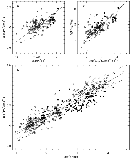
Figure 18: a Size-linewidth plot for the clumps found in the CO datasets of WB89 85 (open squares), WB89 380 (open triangles) and WB89 437 (filled circles) plotted together. The drawn line indicates the linear least squares fit to the data. b As a, but with additional data: inner Galaxy (open circles) and outer Galaxy (filled triangles) from BW95; Rosetta nebula (lower-resol. data; stars) and Orion (asterisks) from this paper; Taurus (filled squares) from Ungerechts & Thaddeus unger (1987); High-latitude clouds (crosses) from Heithausen et al. heith (1993). The drawn line is a least-squares bisector fit through all datapoints; the dashed line is a fit to outer Galaxy and BIMA data; the dotted line is a fit to the inner Galaxy and local cloud data (Taurus, RMC, HLCs, Orion). c Plot of the virial mass versus the CO luminosity for clumps in all three objects. The full line is the linear least squares fit to our data; the short-dashed line is the fit based on the BW95 data for inner Galaxy clouds; the long-dashed line (practically invisible, because coincident with the drawn line) is the fit to BW95 data for outer Galaxy clouds.

5 Discussion

5.1 CO clump properties

5.1.1 Size-linewidth relation

Fig. 18a shows the size-linewidth plot of the CO-clumps in all three sources. The data cover a narrow range in size, and a weak correlation between these two parameters is revealed. The formal linear-least-squares fit to the data gives:

$${\rm\log}\Delta v=(0.41\pm 0.02)+(0.75\pm 0.04)\log r$$ (1)

(corr. coeff. 0.61; for all fits in this paper we used the bisector fit: see e.g. Isobe et al. isobe (1990)). This is considerably steeper than the size-linewidth relations found for samples of molecular clouds (see e.g. BW95; Blitz blitz (1993) for an overview), and is probably due to the small range in radius. A similar effect was noted by BW95, who from a fit to 112 outer Galaxy clouds found a slope of 0.53$\pm$0.03 (corr. coeff. 0.79), while the individual datasets of which their total sample was composed, gave slopes between 0.39$\pm$0.05 and 0.79$\pm$0.13. To illustrate this point, Fig. 18b shows the data from Fig. 18a in the context of a larger data set; the data are essentially from BW95, augmented by additional data from the literature (see caption) to bridge the gap in radius between the present data and those of BW95. It is clear that the present data are consistent with the range defined by the fits made to inner- and outer Galaxy data. A fit through all data points in this figure leads to

$$\log\Delta v=(0.21\pm 0.01)+(0.44\pm 0.01)\log r$$ (2)

(corr. coeff. 0.93).

In Fig. 18b we have mixed data for whole clouds with data for clumps within clouds (Taurus, RMC). In fact, size-linewidth relations derived for clumps show a range of slopes similar to what is found for samples of clouds. For our comparison sample we find 0.74$\pm$0.09 (corr. coeff. 0.61) and 1.03$\pm$0.09 (corr. coeff. 0.76) for the RMC and Orion, respectively. Carr (carr (1987)) derives 0.24$\pm$0.06 for ¹³CO clumps in Cep OB3, while Loren (loren (1989)) finds that $\Delta v$ is independent of size for ¹³CO clumps in $\rho$Oph. And finally, Lada et al. (lada (1991)), from CS data, find that the size-linewidth relation depends on clump definition. They, like others before them (Issa et al. issa (1990); Combes combes (1991)) cast doubt on whether this relation really reflects the dynamical state of molecular clouds.

Fig. 18c shows the virial mass of the clumps as a function of the CO luminosity. The drawn line is a fit to these data, while the dashed lines are fits to data for inner- and outer Galaxy clouds (BW95; see caption). A good correlation is found between the virial mass and the CO luminosity:

$$\log M_{\rm vir}=(1.13\pm 0.04)+(0.90\pm 0.05)\log L_{\rm CO}$$ (3)

(corr. coeff. 0.70), virtually identical to the fits obtained for inner- and outer Galaxy clouds as a whole (BW95). As was shown by BW95, the lack of an offset between inner- and outer Galaxy clouds in a diagram of $\log L_{\rm CO}$ and $\log\Delta v$ (which is similar to what is shown in Fig. 18c) implies that there is no indication of a change in $X$ (= $N{\rm(H_{2})}/W_{\rm CO}$) between inner- and outer Galaxy. Fig. 18c shows that what applies to entire clouds also holds for clumps. We note however that BW95 also concluded that a $\log L_{\rm CO}$ vs. $\log\Delta v$ (or $\log M_{\rm vir}$) diagram may not be the correct instrument from which to actually derive a value of $X$.

Figure 19: Plot of the clump mass distribution: log(d$N$/d$M$) vs. log$M$ a WB89 85 and WB89 380 (shifted down by –2.0). The dashed lines indicate linear least squares fit to the data above 4 and 6 M_⊙, respectively for WB89 85 and WB89 380. b as a, for Orion, RMC (low-resolution data; shifted down by –1.5), and RMC (high-res. data; shifted down by –3). The dashed lines are fits to the data above 2, 126, and 8 M_⊙ respectively, for Orion, RMC (low-res.), and RMC (high-res.).

5.1.2 Mass distribution

An important parameter describing clumps in molecular clouds is the shape of their mass distribution. Many different studies of nearby (see e.g. Combes combes (1991)) and distant (BW95) molecular clouds have found very similar mass distribution slopes between $-1.4$ and $-1.8$ in a plot of log(d$N$/d$M$) vs. log$M$. Interestingly enough, the same slopes are found for the mass distribution of clumps inside clouds (e.g. Kramer et al. (1998b ), who studied the clumps in 7 clouds, with a range in masses and resolution, and found slopes between $-1.6$ and $-1.8$). Fig. 19 shows the mass distribution for the clumps in WB89 85 and WB89 380, as well as for the clumps in the comparison clouds RMC (lower-resolution data) and Orion B South. For WB89 85 a fit to the data for $M>4.0$ M_⊙ results in a mass distribution with slope $-1.28\pm 0.05$. For WB89 380 the slope of a fit to the mass distribution for $M>6.3$ M_⊙ is $-1.49\pm 0.25$. The slopes derived for these two outer Galaxy clouds are somewhat on the low side compared to the literature values quoted above, i.e. the mass distributions are slightly flatter than what is found in most local clouds. In part this may be due to the uncertainty introduced by the small number of clumps in these clouds. If real, this discrepancy might be interpreted as an indication that (these) outer Galaxy clouds would form relatively more massive stars than local clouds. However, fits to the mass distributions of the RMC (high-res.; for $M>7.9$ M_⊙), RMC (low-res.;for $M>126$ M_⊙) and Orion B South (for $M>2.0$ M_⊙) yield slopes of $-1.55\pm 0.03$, $-1.24\pm 0.09$ and $-1.14\pm 0.05$, respectively, the latter two of which are also flatter than the values found in the literature. In particular, Kramer et al. (1998b ), found a slope of $-1.72\pm 0.09$ for Orion, using the same dataset, but a different clump-finding routine GAUSSCLUMPS, though we note that many clumps in their list are found lying on and in part beyond the edge of the mapped region, or appear to be unresolved, and therefore ought to have been excluded from their fit. A similar lowish value is found for Maddalena’s Cloud (G216$-$2.5; $-$1.4) by Williams et al. (williams (1994)), using the same clump finding method as we do here, which suggests this may be due to the properties of CLUMPFIND. Compared to GAUSSCLUMPS, and compared to derivations of mass spectra of ensembles of clouds (rather than of clumps within a cloud), CLUMPFIND tends to underestimate the number of low-mass clumps, lumping them with the more massive ones, thus giving rise to shallower mass spectra (Kramer et al. 1998b ). The fact that we have used only resolved clumps in the derivation of the mass spectra will strenghten this tendency, because the unresolved clumps will also be the ones with the lowest mass. On the other hand, GAUSSCLUMPS finds small clumps that may not be real, but parts of larger non-Gaussian clumps. However, neither in the outer Galaxy clouds, nor in the local clouds, is the slope of the mass distribution the same as that of the IMF (i.e. $-$1.5 for stars of mass $1-10$ M_⊙ and $-$2.3 for stars of mass $>10$ M_⊙; Miller & Scalo miller (1979)). For outer Galaxy clouds this situation is even more critical in view of those studies (Garmany et al. garmany (1982); Wouterloot et al. wouterfieg (1995)) that find that at $R>R_{0}$ the slope of the IMF becomes steeper, resulting in an even larger difference with the values found here. One can think of several ways in which the observed clump mass spectrum can evolve into the IMF: The process of star formation is always accompanied by phases of mass loss; if the mass that is being shed increases with the mass of the star being formed, this will steepen the slope of the mass distribution. Alternatively (or in addition), the clumps may contain smaller sub-clumps (that are so far unresolved), the mass distribution of which may approach that of the IMF; and/or the clumps we have detected will undergo further fragmentation before star formation sets in.

Figure 20: Physical parameters of the CO clumps as a function of mass for two outer Galaxy clouds (left) and two local clouds (right). Symbols are for WB89 85 (open squares), WB89 380 (open triangles), Orion B South (crosses), and the RMC low-resolution (open circles) and high-resolution data (stars). The following parameters are shown: a, b The mean clump gas density $\bar{n}_{\rm H}$; c, d The turbulent pressure $P_{\rm turb}$/k; e, f The pressure due to the self-gravity of the clump, $P_{\rm grav}$/k; g, h The virial parameter $\alpha$ (=$P_{\rm turb}/P_{\rm grav}$).

5.1.3 Physical parameters

We shall compare several parameters of the clumps in the outer Galaxy clouds with those in the local comparison sample.

The total kinetic energy of a clump is $E_{\rm kin}=3/2M_{\rm CO}\sigma^{2}$, where $\sigma$ is the one-dimensional velocity dispersion, which includes both the thermal and turbulent components. The gravitational energy, assuming a spherical mass distribution with density $\rho\propto r^{-2}$ is $E_{\rm grav}$ = – G $M_{\rm CO}^{2}/r$. The magnetic energy, due to a field of strength $B$, is $B^{2}$/8$\pi$. The virial theorem for a clump, with external pressure $P$, can then be written as

$$4\pi r^{3}P=3M_{\rm CO}\sigma^{2}-{\rm G}M_{\rm CO}^{2}/r+B^{2}/8\pi$$

(after Fleck fleck (1988)). From this we find

$$P/{\rm k}=\bar{\rho}\sigma^{2}/{\rm k}-{\rm G}M_{\rm CO}\bar{\rho}/3r{\rm k}+B^{2}/8\pi{\rm k},$$

where $\bar{\rho}=(3/4\pi)M_{\rm CO}r^{-3}$ is the average mass density. The first term on the right-hand side in this equation is the pressure due to the motions of the molecules in the clump, $P_{\rm turb}$/k (which we shall call ‘turbulent pressure’, because the non-thermal contribution to $\sigma$ dominates); the second term is the gravitational pressure $P_{\rm grav}$/k, and the last term is the magnetic pressure $P_{\rm magn}$/k. These terms can be written as follows:

$$P_{\rm turb}/{\rm k[Kcm^{-3}]}=29.66\times\bar{n}_{\rm H}\,\Delta v^{2},$$

with $\bar{n}_{\rm H}{\rm[cm^{-3}]}=\bar{\rho}/\mu_{\rm H}=7.12\times M_{\rm CO}{\rm[M_{\odot}]}\,r{\rm[pc]}^{-3}$, the average volume density of nucleons, $\mu_{H}$ the mass of a hydrogen atom, corrected for a contribution of He (a factor 1.36), and $\Delta v$ [kms^-1] the FWHM line width, and

$$P_{\rm grav}/{\rm k[Kcm^{-3}]}=0.236\times M_{\rm CO}{\rm[M_{\odot}]}\,\bar{n}_{\rm H}{\rm[cm^{-3}]}\,r{\rm[pc]}^{-1}.$$

This last term can also be written in terms of the surface density $\Sigma$ (= $M/\pi r^{2}$): $P_{\rm grav}/{\rm k=(G\pi/k)}\times\Sigma^{2}$, or

$$P_{\rm grav}/{\rm k[Kcm^{-3}]}=16.58\times\Sigma[M_{\odot}{\rm pc}^{-2}]^{2}.$$

The ratio of the turbulent and the gravitational pressures is

$$\alpha=3r\sigma^{2}/{\rm G}M_{\rm CO}=126\,r{\rm[pc]}\,\Delta v[{\rm kms}^{-1}]^{2}/M_{\rm CO}[{\rm M}_{\odot}],$$

which is identical to the ratio between $M_{\rm vir}$ and $M_{\rm CO}$, and is usually called the virial parameter (see e.g. Bertoldi & McKee bertoldi (1992)). If a clump is in virial equilibrium with external surface pressure $P$=0, and in the absence of a magnetic field, then the turbulent pressure is exactly balanced by the gravitational pressure, $\alpha=1$, and $M_{\rm CO}$ = $M_{\rm vir}$. If the kinetic energy is exactly balanced by its gravitational energy, $E_{\rm kin}$ = G$M_{\rm CO}^{2}/r$, then its mass is $M_{\rm CO}=3r\sigma^{2}/2{\rm G}=0.5\times M_{\rm vir}$; the cloud is then called gravitationally bound.

The magnetic pressure can be written as

$$P_{\rm magn}/{\rm k[Kcm^{-3}]}=288.3\times B[\mu{\rm G}]^{2}.$$

In Fig. 20 we have plotted the clump parameters derived above, as a function of clump mass. In this figure, the panels on the left-hand side are for the outer Galaxy clouds, while those on the right-hand side are for the local comparison clouds. The average densities of the clumps in the local clouds lie more or less between 10² and 10⁴ cm^-3, with the clumps found in the high-resolution IRAM 30-m RMC maps having the highest values at a fixed mass; for the clumps in our outer Galaxy sample, the density ranges between $4\times 10^{2}$ and $4\times 10^{4}$ cm^-3, with those in WB89 380 having the highest values. WB89 380 has been observed at the highest spatial resolution, and has more clumps with smaller radii; the density $\bar{n}_{\rm H}\propto M_{\rm CO}\times r^{-3}\propto r^{-1}$, and thus higher densities can be expected. For the majority of clumps in the outer Galaxy clouds, the turbulent gas pressure ($10^{4}-10^{6}$ Kcm^-3; panel c) and the pressure due to self-gravity ($10^{3}-10^{6}$ Kcm^-3; panel e) are both higher than those in local clumps at comparable mass. Also here, for the local clouds at fixed clump mass, the highest pressures are for the higher-resolution RMC clumps. The virial parameter, i.e. the ratio of turbulent (trying to disperse the clumps) and gravitational (working to keep them together) pressure (panels g, h), also shows a different distribution in both cloud samples. The most massive clumps in both outer Galaxy- and local clouds have $\alpha\approx$1, i.e. there is equilibrium between $P_{\rm turb}$ and $P_{\rm grav}$, but for the lower-mass clumps the turbulent pressure is the larger one, and $\alpha$ increases with decreasing clump mass, implying that the lower-mass clumps would need some external pressure if they are to be confined. The important thing to note, however, is that in the outer Galaxy clouds there are a number of low-mass clumps (down to the lowest masses found; a few M_⊙) where self-gravity is the dominating force balancing the internal turbulent pressure (i.e. $\alpha\approx$1), which suggests that these are potentially star-forming clumps. We shall return to this interesting fact later.

5.1.4 Clump stability and implications for the IMF

After the general considerations presented in Sect. 5.1.3, in this section we consider the stability of the clumps, i.e. we look at the balance between the various pressure terms (those trying to expand the clump, and those working to compress it).

Figure 21: Ratio of the pressures balancing a clump’s equilibrium for clumps in outer Galaxy clouds (left-hand panels) and in local clouds (right). Symbols are as follows: WB89 380, open triangles; WB89 85: open squares. Orion B South: crosses; RMC lower-resolution data: open circles; RMC higher-resolution data: stars. a, b Ratio of turbulent and gravitational pressures; c, d As a, b but the gravitational pressure is the sum of the pressure due to the clump’s self-gravity, and the pressure on the clumps exerted by the cloud’s interclump gas, as a consequence of the self-gravity of the cloud as a whole; e, f As c, d, but the pressure term of a 10$\mu$G magnetic field has been added to the turbulent pressure.

A molecular cloud is an ensemble of relatively high-density clumps, which are moving about in a low-density (interclump) medium. Both the movement of the clumps and the gravitational force of the molecular cloud material exert pressures on the interclump medium. If the cloud as a whole is in equilibrium, these pressures are of comparable magnitude and work in opposing directions. The clumps themselves are also subject to various pressures. The thermal and (the larger) turbulent motions of the molecular material within them seek to expand the clumps, while their self-gravity and the pressure of the surrounding interclump medium work against this. The clumps are likely to be threaded by a magnetic field, which also opposes compression (at least perpendicular to the field lines).

$P_{\rm turb}$ and $P_{\rm grav}$ for the individual clumps were calculated and shown in Sect. 5.1.3 (Fig. 20). The interclump pressure may be calculated by assuming that it is in equilibrium with the gravitational pressure exerted by the cloud as a whole. This is in some sense dependent on the pressure of the general ISM surrounding the clouds, which is about 10–20 times lower at $R\approx 17$ kpc as it is in the solar neighbourhood (BW95). This lower pressure allows outer Galaxy clouds to relax to a larger radius than clouds of the same mass at smaller $R$ (BW95), and because the gravitational pressure of a cloud depends also on its radius, the general ISM pressure influences the pressure of the interclump gas. For the clouds under consideration here, this pressure is of the order of several $10^{4}$ Kcm^-3: $P_{\rm grav,cloud}$/k $\approx 3.7\times 10^{4}$ Kcm^-3 (WB89 85), $1.7\times 10^{4}$ Kcm^-3 (WB89 380), $4.4\times 10^{4}$ Kcm^-3 (Orion), and $5.9\times 10^{4}$ Kcm^-3 (RMC). For the outer Galaxy clouds we considered the mass and radius of the region in which the BIMA observations were carried out, rather than the mass and radius of the entire cloud as detected with KOSMA (a similar procedure has been applied to the Orion and Rosette clouds).

Typical values of the magnetic field in molecular clouds are of the order of a few 10$\mu$G (Troland & Heiles troland (1986)), which leads to $P_{\rm magn}$/k $\approx 2.9\times 10^{4}$ Kcm^-3.

In Fig. 21 we look at the combination of these pressures that influence the stability of a clump. Here we first show (Fig. 21a, b) the ratio of the clumps’ turbulent pressure and the pressure due to their self-gravity. The situation is the same as what is shown in Fig. 20g, h and has been described in Sect. 5.1.3. In Fig. 21c, d we plot the ratio of the former and the total gravitational pressure, i.e. including that which is exerted by the cloud as a whole, through the interclump medium, which shows the consequences on the pressure balance of including an external pressure term. Figs. 21c, d demonstrate that when the pressure of the interclump medium is also taken into account, virtually all clumps are in or close to equilibrium, i.e. the clumps’ own gravity and that of the cloud as a whole, are balanced by the clumps’ turbulent pressure. In fact, for many clumps in the local sample the interclump pressure is much larger than the turbulent pressure. Taken at face value this would suggest large-scale clump collapse and star formation, which is clearly not what we observe, and to prevent large-scale collapse a stabilizing agent is clearly needed. It is also clear that the influence of the interclump pressure on outer Galaxy clumps is smaller than on the local clumps. This is because the interclump pressure is of the same order in both outer and inner Galaxy clouds, but $P_{\rm turb}$ is larger in the outer Galaxy clumps.

Figs. 21e, f show the consequence of adding the pressure term due to a 10$\mu$G magnetic field: for nearly all clumps equilibrium has been restored, with respect to the situation shown in Figs. 21c, d. It may be that the actual value of the magnetic field is larger, especially in the more massive clumps and in the local clouds, but already with the presently used low value it is clear that the magnetic field is an important ingredient in the pressure balance.

From what we have found in Fig. 21a, b, and from the behaviour of the virial parameter $\alpha$ in Figs. 20g, h, it appears that in these outer Galaxy clouds gravity may be the dominant force down to a lower mass than in local clouds. In fact, a closer look at Figs. 20g, h reveals that in the IRAM-RMC data the lowest-mass clump with $\alpha\leq 2$ has $M\approx 23.4$ M_⊙, while this is 2.0 M_⊙ and 4.7 M_⊙ in WB89 380 and WB89 85, respectively, i.e. up to an order of magnitude smaller. Moreover, in WB89 380 there are 14 clumps with $M<23.4$ M_⊙ and $\alpha\leq 2$; in WB89 85 there are 5 clumps that fall within these constraints. This implies that gravitational collapse and star formation may occur more readily even in the smallest of these outer Galaxy clumps. Since a clump of mass $M$ can only form stars of mass less than $M$, this would mean that an excess of low mass stars is expected to form in the outer Galaxy with respect to local clouds. This would provide an explanation for the results of Garmany et al. (garmany (1982)), and Wouterloot et al. (wouterfieg (1995)) who found that the IMF steepens in the outer Galaxy.

We note that in the above, notably in Figs. 18a, and 20, there is a separation between the data for WB89 380 and WB89 85: at the same $\Delta v$, the majority of WB89 380 clumps have a smaller radius than the WB89 85 clumps, while at identical $M_{\rm CO}$ they have a higher density, and a higher internal pressure. A naive interpretation is that this illustrates the difference in evolutionary stage between the two clouds: the younger one, WB89 380, has mostly smaller, higher density clumps, that are on the brink of gravitational equilibrium, and are about to form stars, while the older region WB89 85 has been left with lower-density, more stable clumps (except perhaps for the most massive ones). However, there is a resolution effect to consider: the WB89 85 cloud was observed with a beam size of $0.60\times 0.47$ pc², and a map was constructed on a grid with 0.11 pc spacing; CLUMPFIND looked for clumps with a resolution of 0.22 pc in both coordinates (2$\times$2 grid resolution elements); WB89 380 was observed with a beam of $0.36\times 0.23$ pc², a map was constructed on a grid with 0.11 pc spacing, and clumps were searched with a resolution of 0.14$\times$0.07 pc² (2$\times$1 grid resolution elements), and thus CLUMPFIND can come up with smaller clumps in WB89 380. The same effect is found in the local clouds, from the Williams et al. (willblitz (1995)) RMC observations, via Orion, to the Schneider et al. (schneider (1998)) RMC observations, there is an increase in resolution, and a corresponding shift in the distributions of the data points towards smaller radii and masses, and (at fixed mass) towards higher densities and pressures. The grid-resolution of the Schneider et al. data (0.12 pc) is comparable to that of WB89 85 and WB89 380, but the beam size of the Schneider et al. observations (0.09 pc) is smaller, though close to that of the WB89 380 observations.

The question is now, whether the difference we see in Figs 20g, h between outer Galaxy and local (especially the IRAM-RMC) clumps is also a consequence of resolution. Resolution will certainly play a role, as can be seen from the difference in distributions for the RMC high- and low-resolution data, and Orion. Whether resolution is the only explanation is more difficult to say, because this would imply having to demonstrate that the type of clumps (of this size and mass) we see in the outer Galaxy clouds (and then especially in WB89 380) could also be seen in the high-resolution RMC data. We consider the following: in spite of the IRAM beam being smaller than (with respect to the WB89 85 observations) or comparable to (with respect to the WB89 380 observations) those used in the BIMA observations, we do find clumps of comparable mass at the low end of the mass spectrum. The smallest clump mass found in the IRAM-RMC data has $M\approx 3.2$ M_⊙ (cf. 3.3 M_⊙ in WB89 85, and 2.0 M_⊙ in WB89 380). A plot of radius versus mass (not shown) shows that at fixed mass, the radii of the IRAM-RMC clumps is larger than those of WB89 380 clumps (in spite of the IRAM beam being smaller than the BIMA beam), and similar to those of WB89 85 clumps, while the linewidths are comparable. Only at $M<10$ M_⊙ the linewidths of the WB89 380 clumps are smaller. As a consequence, at fixed mass, $\alpha=M_{\rm vir}/M_{\rm CO}$ is smaller for the WB89 380 clumps than for the IRAM-RMC clumps, giving rise to the effect seen in Figs. 20g, h.

Masses for the outer Galaxy clumps have been calculated using the empirical method of $M_{\rm CO}=X\times\int T{\rm d}v$, where for $X$ we have used the local value of 1.9 $\times 10^{20}$ (Kkms^-1)^-1cm^-2. In BW95 we argued that even in the far-outer Galaxy this results in masses equal to LTE masses (derived from ¹³CO observations) if the latter are calculated using the [¹³CO]/[H₂] abundance appropriate for that region of the Galaxy. This is in contrast to claims found in the literature, which would have $X$ at large distances from the galactic center $\sim$2–4 times larger than the local value (e.g. Digel et al. digel (1990); May et al. may (1997)). If for the sake of argument we would adopt an $X$-value of three times the local value, while $r$ and $\Delta v$ remain the same (these are $X$-independent of course), we find that virually all clumps in WB89 380 have $\alpha\leq 2$, while the lowest clump mass is still only 6 M_⊙, i.e. almost 4 times smaller than the lowest clump mass in the IRAM-RMC observations having $\alpha\leq 2$, and thus still resulting in the same conclusion, namely that in (these) outer Galaxy clouds gravity is the dominant force down to a lower mass than in (these) local clouds.

While for the outer Galaxy clumps we arrive at equivalent LTE masses through the use of $X$, LTE masses for the local clumps were derived directly from the column densities of ¹³CO, and are not expected to show a systematic difference with respect to the masses of the outer Galaxy clumps. A potentially serious caveat is whether ¹²CO observations allow one to accurately identify clumps (compared to ¹³CO), i.e. density rather than temperature enhancements. An indication of this is perhaps given by the fact that the CO and CS clumps in general do not coincide. This may however be because in CS we might not be seeing clumps at all, but rather different parts of the expanding shell (see Sect. 3), that show up at different velocities, hence giving the impression of clumpy structure where none may exist. It may also be due to the different excitation conditions of these molecules. In fact, from a (low-resolution) CO survey of GMCs near Cas A and NGC 7538, Ungerechts et al. (ungerechts (2000)) find that the distribution of ¹²CO and ¹³CO is very similar, and that the $\int T{\rm d}v$ of both molecules are closely correlated at each grid point in the map. Radii derived from ¹³CO observations are usually smaller, however, as are the line widths (though not necessarily so in a turbulent medium; see Ungerechts et al. ungerechts (2000), who also find that $M_{\rm vir}$ from ¹²CO and ¹³CO agree within a factor of two), affecting most parameters derived here. Whether ¹³CO-derived radii are smaller than those derived from ¹²CO, also depends on the relative sensitivity of the observations. In the inner Galaxy, the antenna temperature ratio of ¹²CO/¹³CO $\approx$3 (Gordon & Burton gordon (1976)); the (2–1)/(1–0) line ratios are approximately unity. The 2.5$\sigma\sim 1.3$ K limit used in the clumpfind procedure for the high-resolution RMC ¹³CO data would correspond to $T(^{12}$CO) of about 4 K. According to BW95 there is no gradient in the mean cloud antenna temperature with distance from the galactic center, and it should be possible to compare this temperature directly with that which we used as limiting value for the clumpfind procedure in the outer Galaxy clouds, viz. 3.3 K for WB89 85 and 8.7 K for WB89 380. From this we see that WB89 85 and the IRAM-observations of the RMC are compatible, while we go less deep in the case of WB89 380. This might result in seeing only the ‘tips of the icebergs’ in WB89 380, i.e. finding only the peaks of the clumps, resulting in fewer clumps, which are also smaller and less massive than they would be, had we been able to search down to a lower level. To check how this influences our results, we ran a clumpfind-test on the WB89 85 data, using the same limiting value as we have for WB89 380, i.e. 8.7 K. As expected, CLUMPFIND now finds fewer clumps (34, 12 of which are considered useful [resolved and not at the edge of the map]). The new clumps are found at the positions of the most massive clumps from our original analysis of this cloud, with masses, radii, and line widths for most clumps larger than the clumps originally found at these positions. In a mass-radius plot the old and new data points overlap. The clump with the lowest mass has $M_{\rm CO}\sim 19$ M_⊙, and $\alpha\sim 3$. The others have masses between 84.5 and 586 M_⊙, and $\alpha$ between 0.7 and 2.1. Because we do not find smaller and less massive clumps by going less deep, this result strengthens the conclusion that the difference found between the high-resolution RMC results and those of the outer Galaxy clouds is not due to the fact that different transitions were observed, nor due to sensitivity.

In spite of the arguments presented above, it is clear that comparing such different data sets is not a straight-forward matter, because many effects play a role. One would need to study a sample of local and outer Galaxy clouds with carefully selected telescopes, in the same transitions and analyzed in the same way. The cloud sample should preferably be selected taking into account $L_{\rm fir}$ of the IRAS source, and evolutionary status, to ensure that as little bias as possible is introduced.

6 Summary

The fields around luminous IRAS point sources in three molecular clouds in the outer Galaxy have been observed in CO (1–0) and CS (2–1) using the BIMA interferometer. These observations were combined with single dish data from the NRAO 12-m and the IRAM 30-m telescopes. Using this technique we were able to obtain maps around these sources, of about 6 pc in diameter with a resolution of about 0.2 pc. This enables us to analyse small-scale properties of the molecular gas on scales similar to the smallest size-scales on which clump properties of molecular clouds in the solar neighbourhood are studied. The data sets have been analyzed using an automated three-dimensional clump-finding and -analysis program.

From the CO data we find a size-linewidth relation that is steeper than what is found in nearby molecular clouds. This can be explained by the rather narrow range in radius for the clumps in our data set (Sect. 5.1.1). From the CO data we find a somewhat shallower clump mass distributions than in nearby clouds, with slopes of $-1.28\pm 0.05$ (WB89 85) and $-1.49\pm 0.25$ (WB89 380) in plots of log(d$N$/d$M$) vs. log$M$. However, these slopes are consistent with those found by Williams et al. (williams (1994)) for the RMC and G216$-$2.5 (Maddalena’s Cloud), derived from clumps identified with the same method as used here, and is possibly due to the fact that this method tends to underestimate the number of low-mass clumps, resulting in shallower mass distributions (Sect. 5.1.2).

In Sect. 5.1.3 and 5.1.4 we look in detail at the equilibrium of the clumps both in the two of the outer Galaxy clouds (WB89 85 and WB89 380) and in two local comparison clouds (RMC and Orion B South). The most notable finding is that for outer Galaxy clumps down to the lowest (a few M_⊙) masses found turbulent and gravitational pressure are in equilibrium (virial parameter $\alpha\approx 1$). For clumps in the local clouds this is only so for the more massive (a few tens of M_⊙) ones. Adding the pressure of the interclump medium and that, due to the magnetic field (using a representative value of 10 $\mu$G) to the equation, brings virtually all clumps in the clouds under consideration into equilibrium. We note that the interclump pressure in the outer Galaxy clouds has relatively less influence on the balance, compared to the local clouds, because in the outer Galaxy clouds $P_{\rm turb}$ of the clumps is several times larger than in the local clumps, while the interclump pressure is of the same magnitude.

These results indicate that in these outer Galaxy clouds gravity may be the dominant force down to a much lower mass than in local clouds, implying that gravitational collapse and star formation may occur more readily even in the smallest outer Galaxy clumps. As this leads to the formation of relatively more low-mass stars, it would provide an explanation for the observed steepening of the IMF in the outer Galaxy.

The results presented above are necessarily based on an inhomogeneous dataset, and a comparison between local and outer Galaxy clouds ought to be repeated with a more carefully selected sample using a uniform method of analysis. The potential importance of the conclusion based on the present data makes such a renewed study worthwhile.

Table 3: CO Clump parameters of WB89 85. Right ascension and declination are in arcsecond offsets from the central position of the map: $(\alpha,\delta)_{1950}$ = (21^h 27^m 5$\aas@@fstack{s}$9 , +54° 23′ 42″).

Clump	$\Delta$RA	$\Delta$Dec	$V_{\rm lsr}$	$T_{\rm peak}$	$T_{\rm ave}$	$r_{\rm eff}$	$\Delta v_{\rm fwhm}$	$M_{\rm CO}$	$M_{\rm vir}$
	[″]	[″]	[km s-1]	[K]	[K]	[pc]	[km s-1]	[M⊙]	[M⊙]
(1)	(2)	(3)	(4)	(5)	(6)	(7)	(8)	(9)	(10)
1	24.	50.	-92.50	57.3	23.2	0.65	1.48	349.0	179.0
2	28.	52.	-93.00	54.7	25.7	0.43	1.05	105.0	59.7
3	30.	52.	-93.50	44.4	17.7	0.70	1.28	221.0	145.0
4	8.	36.	-93.00	40.0	15.3	0.77	2.10	336.0	428.0
5	58.	-24.	-94.00	39.6	16.8	0.42	1.33	96.8	93.6
6	58.	-30.	-94.50	37.1	20.3	0.33	1.44	101.0	86.2
7	52.	-32.	-95.75	36.0	17.3	0.55	1.06	104.0	77.9
8	54.	-38.	-95.00	35.1	17.2	0.47	1.43	116.0	121.0
9	-22.	-52.	-93.50	34.4	15.8	0.70	1.37	210.0	166.0
10	12.	40.	-94.00	33.0	13.8	0.91	1.48	275.0	251.0
11	-20.	-32.	-93.75	32.9	13.9	0.74	1.79	294.0	299.0
12	60.	-42.	-96.50	29.0	15.8	0.32	1.06	78.7	45.3
13	48.	-24.	-96.25	25.4	9.4	0.89	1.56	154.0	273.0
14	4.	-4.	-92.50	23.7	7.8	0.88	2.11	179.0	494.0
15	54.	-30.	-96.75	21.8	11.2	0.38	0.96	49.3	44.1
16	-58.	-48.	-93.50	20.5	8.8	0.34	1.26	44.2	68.0
17	-4.	-54.	-95.50	20.0	9.4	0.55	1.25	79.6	108.0
18	36.	56.	-91.25	17.2	9.8	0.42	1.33	33.3	93.6
19	-42.	-44.	-92.75	16.5	9.0	0.57	1.47	79.4	155.0
20	-6.	44.	-92.75	16.3	7.3	0.74	1.68	103.0	263.0
21	58.	-46.	-91.50	16.0	7.5	0.15	1.09	15.6	22.5
22	28.	44.	-95.75	15.8	7.3	0.70	1.26	57.0	140.0
23	-42.	58.	-88.25	15.0	6.9	0.10	0.43	4.7	2.3
24	50.	-50.	-94.25	15.0	6.9	0.56	1.54	45.1	167.0
25	-48.	-56.	-88.25	14.4	6.4	0.16	0.50	5.5	5.0
26	-32.	-50.	-92.50	14.4	7.1	0.53	1.35	34.5	122.0
27	54.	-50.	-92.00	14.3	6.9	0.36	1.23	23.2	68.6
28	56.	-40.	-97.75	13.8	8.2	0.37	0.86	18.4	34.5
29	38.	48.	-90.75	13.4	7.0	0.37	1.16	17.1	62.7
30	-10.	14.	-94.25	13.1	6.8	0.82	1.70	89.6	299.0
31	-32.	26.	-91.50	12.9	6.3	0.61	1.21	42.4	113.0
32	-36.	-14.	-92.75	12.3	5.8	0.75	2.02	70.1	386.0
33	16.	-56.	-95.50	12.1	5.5	0.35	1.09	14.1	52.4
34	-46.	22.	-96.00	11.2	5.2	0.21	0.74	4.9	14.5
35	-58.	46.	-89.25	11.1	5.9	0.14	0.92	4.1	14.9
36	-12.	44.	-91.25	11.0	5.6	0.42	2.37	13.6	297.0
37	-46.	22.	-93.50	10.9	5.3	0.43	0.66	12.1	23.6
38	-14.	12.	-95.00	10.8	5.4	0.35	0.96	11.0	40.6
39	-42.	-6.	-92.25	10.7	5.1	0.49	1.46	19.1	132.0
40	-2.	-58.	-97.00	10.7	5.1	0.26	0.83	5.2	22.6
41	-16.	-28.	-95.50	10.5	5.6	0.77	1.66	44.7	267.0
42	-40.	46.	-88.50	10.4	5.0	0.40	0.84	6.4	35.6
43	12.	-52.	-97.75	10.3	5.2	0.25	0.85	5.0	22.8
44	-6.	42.	-91.50	10.2	6.1	0.58	0.96	20.0	67.4
45	-54.	-10.	-95.75	9.8	5.8	0.38	1.09	16.0	56.9
46	54.	16.	-97.25	9.5	5.5	0.68	1.06	21.6	96.3
47	-36.	44.	-90.25	8.9	4.9	0.46	0.81	7.6	38.0
48	-40.	20.	-94.75	8.9	4.6	0.49	1.01	14.6	63.0
49	4.	-24.	-93.25	8.3	4.5	0.58	2.36	19.8	407.0
50	-26.	18.	-95.00	8.1	4.2	0.33	1.50	5.4	93.6

Table 3: (continued)

Clump	$\Delta$RA	$\Delta$Dec	$V_{\rm lsr}$	$T_{\rm peak}$	$T_{\rm ave}$	$r_{\rm eff}$	$\Delta v_{\rm fwhm}$	$M_{\rm CO}$	$M_{\rm vir}$
	[″]	[″]	[km s-1]	[K]	[K]	[pc]	[km s-1]	[M⊙]	[M⊙]
(1)	(2)	(3)	(4)	(5)	(6)	(7)	(8)	(9)	(10)
51	-12.	16.	-91.50	8.0	4.8	0.79	1.29	37.5	166.0
52	-44.	14.	-97.00	7.9	4.6	0.26	1.46	3.3	69.8
53	6.	-60.	-98.25	7.9	4.7	0.29	0.93	4.4	31.6
54	52.	26.	-98.00	7.9	4.7	0.25	1.09	4.9	37.4
55	22.	36.	-98.25	7.4	4.3	0.44	1.62	5.2	145.0
56	-50.	-2.	-91.25	7.4	4.6	0.28	0.98	3.7	33.9
57	-40.	12.	-95.75	7.3	4.3	0.40	1.41	6.7	100.0
58	-18.	-2.	-95.75	7.3	4.2	0.33	2.42	5.7	244.0
59	-18.	-8.	-96.00	6.9	4.3	0.42	2.88	8.3	439.0
60	-26.	34.	-92.75	6.7	4.3	0.45	0.88	7.0	43.9
61	-44.	22.	-92.50	6.7	4.9	0.38	1.24	13.1	73.6
62	18.	6.	-90.75	6.6	4.6	0.77	1.85	38.3	332.0

Table 4: CO Clump parameters of WB89 380. Right ascension and declination are in arcsecond offsets from the central position of the map: $(\alpha,\delta)_{1950}$ = (1^h 4^m 35$\aas@@fstack{s}$7 , +65° 5′ 21″).

Clump	$\Delta$RA	$\Delta$Dec	$V_{\rm lsr}$	$T_{\rm peak}$	$T_{\rm ave}$	$r_{\rm eff}$	$\Delta v_{\rm fwhm}$	$M_{\rm CO}$	$M_{\rm vir}$
	[″]	[″]	[km s-1]	[K]	[K]	[pc]	[km s-1]	[M⊙]	[M⊙]
(1)	(2)	(3)	(4)	(5)	(6)	(7)	(8)	(9)	(10)
1	38.	18.	-87.00	49.5	24.5	0.28	1.11	56.7	43.5
2	41.	3.	-87.00	45.1	20.4	0.27	1.24	43.0	52.3
3	39.	6.	-87.25	44.7	26.8	0.27	1.01	47.0	34.7
4	42.	-38.	-88.25	41.9	19.4	0.34	1.07	34.4	49.0
5	39.	-3.	-87.50	41.1	21.7	0.25	1.02	31.1	32.8
6	42.	-15.	-87.50	40.3	18.4	0.34	1.04	39.8	46.3
7	6.	-3.	-88.50	39.6	17.3	0.39	1.42	62.4	99.1
8	29.	42.	-87.50	38.9	13.9	0.28	0.90	13.7	28.6
9	39.	0.	-88.00	38.8	19.4	0.32	0.74	27.4	22.1
10	42.	-11.	-87.00	38.3	16.4	0.25	1.24	28.5	48.4
11	42.	-33.	-87.25	37.9	19.7	0.37	1.03	35.7	49.5
12	29.	24.	-87.25	37.5	18.1	0.32	1.53	51.4	94.4
13	6.	-2.	-87.25	36.5	17.8	0.42	1.91	42.3	193.0
14	27.	14.	-87.50	35.9	18.6	0.28	1.07	35.5	40.4
15	9.	-30.	-88.00	35.4	15.4	0.32	1.34	22.8	72.4
16	30.	21.	-88.00	33.6	16.4	0.31	1.20	25.8	56.2
17	12.	-45.	-88.00	33.5	15.8	0.31	1.53	30.8	91.4
18	39.	9.	-88.50	33.3	17.1	0.23	0.72	15.2	15.0
19	17.	3.	-86.50	33.0	17.2	0.29	0.98	24.8	35.1
20	30.	11.	-86.00	32.3	17.6	0.29	1.27	27.3	58.9
21	11.	9.	-87.00	32.0	14.8	0.26	1.64	26.1	88.1
22	23.	2.	-87.00	31.7	14.9	0.35	1.25	29.8	68.9
23	8.	-38.	-88.25	31.6	13.4	0.36	1.34	20.3	81.4
24	-8.	6.	-88.50	31.6	17.0	0.30	1.35	34.0	68.9
25	6.	41.	-87.25	31.2	14.6	0.29	0.75	16.3	20.6
26	3.	9.	-87.25	31.0	17.4	0.28	1.36	31.5	65.3
27	9.	23.	-87.25	30.7	15.8	0.31	1.22	20.3	58.1
28	14.	-44.	-88.75	30.5	15.4	0.21	0.78	9.7	16.1
29	44.	-17.	-86.50	30.2	18.5	0.28	0.80	20.1	22.6
30	-3.	3.	-87.75	30.2	17.2	0.32	1.52	31.7	93.2
31	12.	-27.	-87.50	30.0	17.1	0.42	0.90	35.5	42.9
32	39.	-18.	-84.75	29.5	15.7	0.26	0.93	20.0	28.3
33	11.	23.	-88.00	28.8	16.1	0.32	1.20	29.2	58.1
34	5.	44.	-87.00	28.2	16.2	0.27	0.94	14.5	30.1
35	35.	-12.	-85.75	28.1	13.4	0.28	1.28	18.4	57.8
36	38.	-24.	-85.75	28.0	13.4	0.19	0.95	10.3	21.6
37	26.	35.	-86.50	27.8	16.1	0.43	1.51	59.1	124.0
38	45.	-41.	-86.00	27.5	17.3	0.20	0.86	10.1	18.6
39	6.	18.	-88.00	27.1	15.7	0.26	0.98	20.8	31.5
40	38.	12.	-85.50	27.0	14.6	0.25	1.12	17.7	39.5
41	42.	15.	-85.50	26.9	16.6	0.27	1.41	27.4	67.6
42	39.	-26.	-89.25	26.8	12.9	0.37	1.12	20.2	58.5
43	39.	-17.	-85.50	26.8	14.9	0.24	1.00	13.7	30.2
44	38.	17.	-88.25	26.8	15.9	0.26	0.76	15.8	18.9
45	47.	11.	-88.75	26.7	14.4	0.18	1.36	15.9	41.9
46	30.	-3.	-86.25	26.7	16.0	0.30	1.37	31.4	70.9
47	35.	9.	-84.75	26.4	15.5	0.37	0.96	28.8	43.0
48	44.	-38.	-85.50	26.4	16.1	0.22	0.92	14.3	23.5
49	20.	20.	-87.75	26.3	15.3	0.31	1.47	34.8	84.4
50	30.	-45.	-84.00	26.0	12.8	0.30	1.22	13.9	56.3

Table 4: (continued)

Clump	$\Delta$RA	$\Delta$Dec	$V_{\rm lsr}$	$T_{\rm peak}$	$T_{\rm ave}$	$r_{\rm eff}$	$\Delta v_{\rm fwhm}$	$M_{\rm CO}$	$M_{\rm vir}$
	[″]	[″]	[km s-1]	[K]	[K]	[pc]	[km s-1]	[M⊙]	[M⊙]
(1)	(2)	(3)	(4)	(5)	(6)	(7)	(8)	(9)	(10)
51	14.	5.	-84.00	25.7	15.7	0.49	1.08	37.1	72.0
52	-14.	-33.	-87.00	25.3	12.7	0.27	0.59	8.4	11.8
53	42.	41.	-87.25	24.9	12.8	0.30	1.02	11.7	39.3
54	30.	-5.	-84.50	23.7	12.1	0.33	0.88	15.8	32.2
55	44.	41.	-85.00	22.8	12.6	0.30	0.96	7.9	34.8
56	44.	-33.	-83.50	22.7	12.6	0.22	0.53	4.2	7.8
57	44.	5.	-84.00	22.5	12.9	0.31	1.34	20.2	70.1
58	39.	41.	-84.00	22.1	13.5	0.10	0.69	2.7	6.0
59	36.	36.	-84.00	21.7	12.6	0.23	1.40	9.8	56.8
60	15.	38.	-85.00	21.5	12.1	0.39	1.48	18.2	108.0
61	27.	-8.	-85.25	21.4	12.0	0.17	1.06	5.3	24.1
62	41.	-26.	-84.75	21.3	13.1	0.22	1.06	10.7	31.1
63	18.	-38.	-84.75	21.2	12.0	0.31	1.86	14.0	135.0
64	21.	-27.	-85.50	21.1	12.3	0.21	1.01	6.4	27.0
65	44.	24.	-84.00	21.0	12.5	0.28	1.28	13.2	57.8
66	32.	-30.	-85.50	20.9	12.4	0.23	0.83	8.7	20.0
67	24.	15.	-85.00	20.9	12.3	0.31	0.80	12.6	25.0
68	12.	0.	-82.75	20.8	12.7	0.20	0.68	4.8	11.7
69	33.	-33.	-83.50	20.7	12.9	0.18	1.08	3.7	26.5
70	9.	-12.	-88.00	20.4	12.7	0.37	1.11	24.0	57.4
71	18.	2.	-85.50	20.4	12.4	0.34	0.99	14.3	42.0
72	15.	18.	-86.75	20.4	13.0	0.31	1.08	15.6	45.6
73	45.	15.	-83.25	20.3	12.5	0.22	1.31	6.5	47.6
74	-6.	23.	-87.75	20.2	12.6	0.13	0.44	2.0	3.2
75	29.	15.	-88.50	19.9	12.3	0.29	0.77	9.0	21.7
76	26.	15.	-85.50	19.9	13.5	0.23	0.53	6.2	8.1
77	23.	-36.	-88.25	19.9	12.3	0.33	1.03	15.0	44.1
78	39.	-39.	-89.00	19.8	11.9	0.28	0.90	7.6	28.6
79	42.	30.	-83.25	19.6	12.2	0.23	0.92	6.4	24.5
80	23.	-15.	-86.25	19.6	11.7	0.29	1.13	12.2	46.7
81	12.	2.	-83.25	19.5	12.9	0.44	1.23	20.3	83.9
82	30.	-23.	-86.25	19.4	12.6	0.30	1.53	19.9	88.5
83	27.	-12.	-89.00	19.1	12.0	0.34	1.27	14.6	69.1
84	39.	6.	-89.50	19.0	11.9	0.35	0.66	8.8	19.2
85	2.	14.	-89.00	18.7	12.2	0.32	0.95	13.8	36.4
86	27.	26.	-84.00	18.7	11.9	0.39	1.57	21.7	121.0
87	12.	-18.	-89.00	18.6	12.6	0.24	1.06	6.8	34.0
88	21.	-6.	-85.75	18.6	11.7	0.27	1.37	9.4	63.9
89	14.	-27.	-86.50	18.5	11.6	0.48	1.30	19.0	102.0
90	21.	-42.	-88.50	18.4	12.3	0.18	1.18	6.7	31.6
91	20.	-11.	-88.75	18.4	11.7	0.28	0.85	9.2	25.5
92	-27.	-30.	-89.75	18.2	11.6	0.29	0.65	5.2	15.4
93	21.	11.	-85.25	18.0	12.4	0.29	1.08	17.0	42.6
94	18.	-15.	-89.25	17.9	11.9	0.23	0.99	9.1	28.4
95	18.	-11.	-89.25	17.9	12.5	0.24	0.91	7.4	25.0
96	27.	-12.	-85.00	17.8	10.9	0.20	0.79	5.0	15.7
97	-2.	30.	-87.50	17.5	12.0	0.32	1.44	10.0	83.6

Table 5: CS Clump parameters of WB89 380. Right ascension and declination are in arcsecond offsets from the central position of the map: $(\alpha,\delta)_{1950}$ = (1^h 4^m 35$\aas@@fstack{s}$7 , +65° 5′ 21″).

Clump	$\Delta$RA	$\Delta$Dec	$V_{\rm lsr}$	$T_{\rm peak}$	$T_{\rm ave}$	$r_{\rm eff}$	$\Delta v_{\rm fwhm}$	$M_{\rm vir}$
	[″]	[″]	[km s-1]	[K]	[K]	[pc]	[km s-1]	[M⊙]
(1)	(2)	(3)	(4)	(5)	(6)	(7)	(8)	(9)
1	0.	0.	-86.50	6.4	3.1	0.45	1.57	139.8
2	-2.	12.	-86.80	6.4	3.1	0.51	1.41	127.8
3	2.	10.	-86.20	6.3	3.5	0.38	1.31	82.2
4	4.	6.	-85.30	5.8	3.1	0.50	1.09	74.9
5	4.	-4.	-88.00	5.4	2.9	0.52	1.06	73.6
6	10.	-14.	-87.10	5.1	2.4	0.54	1.45	143.1
7	8.	24.	-88.00	3.9	2.2	0.46	1.16	78.0
8	10.	0.	-83.80	3.8	2.1	0.49	1.81	202.3
9	22.	16.	-85.60	3.4	2.1	0.42	2.42	309.9
10	-16.	-14.	-87.40	3.4	2.0	0.49	2.28	320.9
11	-18.	6.	-87.10	3.4	2.2	0.36	1.51	103.4
12	4.	24.	-85.90	3.3	2.0	0.42	1.90	191.0
13	20.	-12.	-86.80	3.2	2.1	0.36	2.74	340.5
14	-16.	8.	-91.60	3.1	2.1	0.19	0.39	3.6
15	10.	-14.	-86.50	3.1	2.1	0.37	2.06	197.8
16	-16.	22.	-88.30	3.1	2.2	0.42	1.47	114.4

Table 6: CO and CS Clump parameters of WB89 437. Right ascension and declination are in arcsecond offsets from the central position of the map: $(\alpha,\delta)_{1950}$ = (2^h 39^m 30$\aas@@fstack{s}$6 , +62° 44′ 22″).

Clump	$\Delta$RA	$\Delta$Dec	$V_{\rm lsr}$	$T_{\rm peak}$	$T_{\rm ave}$	$r_{\rm eff}$	$\Delta v_{\rm fwhm}$	$M_{\rm CO}$	$M_{\rm vir}$
	[″]	[″]	[km s-1]	[K]	[K]	[pc]	[km s-1]	[M⊙]	[M⊙]
(1)	(2)	(3)	(4)	(5)	(6)	(7)	(8)	(9)	(10)
CO
2	12.	15.	-72.00	33.0	12.1	0.85	1.30	308.0	181.0
3	3.	6.	-73.00	28.5	13.3	0.78	1.55	327.0	236.0
4	24.	15.	-73.25	25.3	8.6	0.86	1.57	267.0	267.0
5	0.	-27.	-72.50	21.2	7.4	0.70	1.56	206.0	215.0
6	-27.	18.	-69.75	18.4	8.5	1.10	2.95	480.0	1206.2
7	-24.	-12.	-72.25	18.3	8.3	0.73	1.80	222.0	298.0
8	0.	6.	-75.75	9.0	3.5	0.83	1.80	63.4	339.0
9	-6.	9.	-65.25	6.1	2.9	0.90	2.22	60.8	559.0
10	0.	6.	-78.25	5.6	2.6	0.71	1.19	24.0	127.0
11	6.	-15.	-75.50	4.6	2.5	0.45	1.55	13.6	136.0
12	9.	9.	-80.25	3.9	2.2	0.60	1.01	9.6	77.1
CS
1	3.	6.	-71.60	6.0	1.8	1.11	1.71	–	409.0
2	6.	6.	-72.50	4.2	1.4	1.02	1.23	–	194.4

Table 7: Clump parameters of RMC low-resolution ¹³CO data. Gal. longitude and latitude are in arcmin offsets from the central position of the map: l, b = 207.^∘5, $-$1.^∘823

Clump	$\Delta l$	$\Delta b$	$V_{\rm lsr}$	$T_{\rm peak}$	$T_{\rm ave}$	$r_{\rm eff}$	$\Delta v_{\rm fwhm}$	$M_{\rm lte}$	$M_{\rm vir}$
	[′]	[′]	[km s-1]	[K]	[K]	[pc]	[km s-1]	[M⊙]	[M⊙]
(1)	(2)	(3)	(4)	(5)	(6)	(7)	(8)	(9)	(10)
1	-30.	0.	15.60	8.6	2.1	2.32	2.19	2510.0	1400
2	-24.	-2.	10.84	6.3	2.0	2.82	1.50	2840.0	799
3	3.	6.	12.88	6.1	2.0	3.00	2.14	2810.0	1730
4	-15.	0.	12.88	6.0	2.2	2.56	2.45	1430.0	1940
5	-14.	-20.	15.60	5.9	1.6	2.79	1.49	1310.0	780
6	-23.	-5.	12.88	5.5	2.4	1.73	1.93	1240.0	812
7	-6.	-8.	16.28	5.3	1.4	2.20	1.73	551.0	830
8	-41.	-11.	16.28	5.2	2.0	1.94	2.02	1000.0	997
9	-44.	-8.	15.60	5.1	2.0	1.27	1.61	387.0	415
10	-39.	-33.	14.24	5.1	1.7	1.98	2.07	901.0	1070
11	-26.	-3.	12.88	5.0	2.1	2.24	1.99	1220.0	1120
12	-24.	-3.	16.28	4.5	1.4	1.91	1.72	508.0	712
13	-21.	2.	12.20	4.5	1.8	1.74	1.98	739.0	860
14	-38.	-5.	14.92	4.5	1.6	2.18	2.43	1160.0	1620
15	17.	3.	11.52	4.3	1.9	2.99	1.57	2510.0	929
16	-9.	-5.	12.20	4.1	1.6	2.88	2.05	1560.0	1530
17	12.	-6.	14.92	3.9	1.6	2.94	2.17	1860.0	1740
18	-35.	14.	14.24	3.2	1.4	0.87	1.57	126.0	270
19	6.	-5.	15.60	3.1	1.2	2.58	2.19	718.0	1560
20	24.	2.	10.84	3.1	1.2	2.49	1.75	506.0	961
21	-9.	24.	12.20	3.0	1.2	2.64	2.05	793.0	1400
22	9.	15.	14.92	3.0	1.1	2.49	2.05	441.0	1320
23	6.	-8.	11.52	2.9	1.1	2.23	2.07	508.0	1200
24	-35.	11.	14.92	2.8	1.0	1.18	1.77	141.0	466
25	-42.	-42.	13.56	2.8	1.1	1.93	1.39	302.0	470
26	-24.	11.	9.48	2.7	0.9	1.25	1.24	105.0	242
27	11.	-6.	11.52	2.5	1.3	2.68	1.84	789.0	1140
28	-3.	33.	13.56	2.3	0.8	2.20	2.07	202.0	1190
29	-8.	33.	14.24	2.3	0.9	1.64	1.50	141.0	465
30	0.	-14.	10.16	2.2	1.0	2.79	2.84	676.0	2840
31	-41.	-15.	14.24	2.1	0.9	2.06	2.79	241.0	2020
32	18.	3.	14.92	2.0	1.0	2.68	1.72	493.0	999
33	21.	14.	10.84	1.9	0.8	1.99	1.96	193.0	963
34	-2.	6.	5.40	1.9	0.9	1.39	1.78	100.0	555
35	0.	3.	5.40	1.6	0.9	1.02	0.85	40.8	92.9
36	-32.	-41.	11.52	1.6	0.9	1.66	1.41	153.0	416
37	-12.	-6.	16.28	1.5	0.7	1.88	2.54	129.0	1530
38	0.	-3.	10.84	1.5	0.9	2.07	2.41	264.0	1510
39	44.	8.	11.52	1.5	0.8	0.52	1.48	18.9	144
40	-35.	-36.	14.24	1.5	0.9	0.94	1.48	73.9	259
41	-5.	27.	6.76	1.4	0.8	2.00	2.13	126.0	1140
42	-11.	-14.	8.12	1.4	0.8	2.12	1.99	199.0	1060
43	-33.	-29.	16.96	1.3	0.9	1.11	0.85	42.4	101
44	41.	-9.	10.16	1.3	0.7	1.57	0.89	60.9	157
45	-12.	-17.	12.88	1.3	0.8	0.78	1.14	50.2	128
46	-26.	-36.	14.92	1.1	0.8	0.70	0.79	15.0	55.1

Table 8: Clump parameters of RMC high-resolution ¹³CO data. Gal. longitude and latitude are in arcsec offsets from the central position: l, b = 207.^∘0154, $-$1.^∘8228

Clump	$\Delta l$	$\Delta b$	$V_{\rm lsr}$	$T_{\rm peak}$	$T_{\rm ave}$	$r_{\rm eff}$	$\Delta v_{\rm fwhm}$	$M_{\rm lte}$	$M_{\rm vir}$
	[″]	[″]	[km s-1]	[K]	[K]	[pc]	[km s-1]	[M⊙]	[M⊙]
(1)	(2)	(3)	(4)	(5)	(6)	(7)	(8)	(9)	(10)
1	-855.	-420.	15.50	17.0	6.7	0.57	1.61	123.0	186
2	-1050.	-420.	20.12	16.2	4.9	0.34	1.25	35.2	66.9
3	-945.	-300.	12.42	11.7	5.3	0.43	0.96	30.1	49.9
4	-945.	-315.	13.08	11.7	5.6	0.44	0.81	23.4	36.4
5	-885.	-315.	13.74	10.8	5.5	0.65	0.98	59.1	78.7
6	-930.	-345.	22.10	7.8	3.2	0.26	1.29	6.6	54.5
7	-915.	-300.	21.66	7.8	3.3	0.31	0.98	8.0	37.5
8	-810.	-330.	20.12	6.7	3.2	0.22	0.87	3.7	21.0
9	-915.	-390.	12.64	5.8	2.6	0.50	1.30	11.0	106
10	0.	-45.	16.38	19.9	5.8	0.66	1.02	87.4	86.5
11	60.	-75.	15.06	19.3	6.6	0.50	1.56	115.0	153
12	30.	-30.	15.06	17.9	10.3	0.41	1.27	88.4	83.3
13	150.	-90.	16.16	13.5	4.3	0.48	0.85	25.7	43.7
14	90.	15.	15.06	13.1	5.8	0.47	1.28	48.5	97.0
15	195.	-105.	15.94	8.1	3.1	0.47	0.95	15.3	53.4
16	195.	-105.	11.76	8.0	3.7	0.52	0.94	24.4	57.9
17	105.	45.	15.28	7.8	3.2	0.41	1.16	14.5	69.5
18	300.	-15.	10.22	6.8	3.5	0.50	1.30	19.2	106.0
19	210.	15.	11.98	6.7	3.2	0.35	0.92	6.9	37.3
20	315.	-75.	10.88	6.7	3.3	0.44	1.16	13.0	74.6
21	165.	0.	11.76	6.6	3.1	0.45	0.99	11.4	55.6
22	30.	-75.	10.66	6.6	3.3	0.44	0.97	12.9	52.2
23	240.	-30.	10.66	6.3	3.3	0.52	0.82	17.1	44.1
24	240.	-105.	12.86	6.2	3.3	0.60	1.01	30.6	77.1
25	105.	-75.	10.22	6.0	3.1	0.34	0.93	7.2	37.1
26	225.	-30.	11.76	5.6	2.9	0.37	0.89	9.2	36.9
27	150.	-90.	11.10	5.5	3.1	0.50	0.81	13.8	41.3
28	120.	0.	10.00	5.5	2.9	0.43	0.94	10.5	47.9
29	75.	-15.	10.00	5.4	2.6	0.31	1.00	4.4	39.1
30	135.	-45.	10.66	5.3	3.4	0.44	0.81	10.6	36.4
31	75.	-105.	10.44	5.2	3.4	0.34	1.07	9.5	49.0
32	210.	0.	13.96	4.5	2.1	0.41	1.20	4.3	74.4
33	105.	45.	9.78	4.3	2.3	0.35	1.07	5.3	50.5
34	225.	-30.	14.18	4.2	2.1	0.42	1.25	5.7	82.7
35	240.	-90.	9.34	3.2	1.9	0.34	1.29	3.2	71.3
36	30.	15.	10.22	3.2	1.8	0.37	0.92	3.5	39.5
37	-1440.	0.	10.00	12.7	5.7	0.44	1.44	49.9	115
38	-1455.	-45.	10.00	11.8	4.6	0.41	1.75	44.4	158
39	-1335.	45.	9.56	8.3	3.7	0.55	1.15	25.2	91.6

Table 9: Clump Parameters of the Orion B South ¹³CO data. Right ascension and declination are in arcmin offsets from the central position of the map: $(\alpha,\delta)_{1950}$ = (5^h 39^m 12$\aas@@fstack{s}$0 , $-$1° 58′ 00″).

Clump	$\Delta$RA	$\Delta$Dec	$V_{\rm lsr}$	$T_{\rm peak}$	$T_{\rm ave}$	$r_{\rm eff}$	$\Delta v_{\rm fwhm}$	$M_{\rm lte}$	$M_{\rm vir}$
	[′]	[′]	[km s-1]	[K]	[K]	[pc]	[km s-1]	[M⊙]	[M⊙]
(1)	(2)	(3)	(4)	(5)	(6)	(7)	(8)	(9)	(10)
1	1.	2.	10.68	15.5	3.6	1.57	2.88	891.0	1641
2	-1.	-21.	10.00	13.5	3.9	1.56	2.40	828.0	1132
3	-7.	10.	8.87	10.7	4.8	1.10	1.90	314.0	500
4	3.	18.	9.10	9.3	4.8	0.81	1.21	101.0	149
5	1.	14.	10.00	7.8	3.1	1.06	2.59	215.0	896
6	10.	-2.	9.78	6.7	3.0	1.29	2.33	304.0	882
7	1.	25.	8.65	6.3	2.8	0.75	1.42	62.6	191
8	9.	-8.	10.45	6.2	3.3	0.70	1.40	59.6	173
9	-11.	-13.	11.58	5.4	2.0	1.36	2.22	146.0	845
10	9.	7.	9.55	5.3	3.3	0.71	1.33	31.0	158
11	9.	23.	9.55	5.0	2.3	0.81	1.64	62.7	275
12	1.	25.	10.91	5.0	2.4	1.10	2.34	112.0	759
13	-6.	21.	9.10	4.6	2.3	0.85	1.62	54.4	281
14	9.	-31.	10.23	3.7	2.3	1.28	2.01	90.2	652
15	9.	-28.	10.00	3.7	2.0	0.70	1.66	25.9	243
16	11.	-26.	9.32	3.3	1.7	1.08	1.87	64.2	476
17	18.	20.	10.45	3.2	1.3	1.19	2.41	54.9	871
18	14.	30.	9.55	3.1	1.5	0.82	1.63	37.5	275
19	19.	22.	9.78	3.0	1.5	0.85	2.44	44.2	638
20	18.	8.	9.55	2.6	1.2	0.74	2.64	28.7	650
21	10.	26.	7.97	2.6	1.1	0.89	1.15	15.1	148
22	16.	8.	10.00	2.5	1.5	0.88	1.09	13.6	132
23	9.	25.	3.90	2.5	1.1	0.40	0.70	2.9	24.7
24	-11.	19.	10.23	2.4	1.4	0.80	2.11	31.6	449
25	4.	25.	13.84	2.4	1.0	0.45	1.20	3.7	81.6
26	8.	-1.	13.39	1.9	1.2	0.60	2.02	5.9	308
27	8.	7.	7.06	1.8	1.1	0.69	1.08	7.0	101
28	19.	22.	3.90	1.8	0.9	0.58	0.94	3.3	64.6
29	9.	-3.	12.26	1.8	1.0	0.72	1.57	7.6	224
30	13.	17.	8.65	1.8	1.3	0.56	1.31	4.0	121
31	7.	9.	5.48	1.6	1.0	0.51	0.90	3.9	52.1
32	-1.	7.	5.48	1.5	0.8	0.65	1.42	5.0	165
33	10.	10.	5.71	1.4	0.8	0.49	1.11	2.5	76.1