Maximum-likelihood method for estimating the mass and period distributions of extra-solar planets

Abstract

We investigate the distribution of mass $M$ and orbital period $P$ of extra-solar planets, taking account of selection effects due to the limited velocity precision and duration of existing surveys. We fit the data on 63 planets to a power-law distribution of the form $dn=CM^{-\alpha}P^{-\beta}(dM/M)(dP/P)$, and find $\alpha=0.12\pm 0.10$, $\beta=-0.26\pm 0.06$ for $M\lesssim 10M_{\mathrm{J}}$, where $M_{\mathrm{J}}$ is the Jupiter mass. The correlation coefficient between these two exponents is $-0.32$, indicating that uncertainties in the two distributions are coupled. We estimate that 3% of solar-type stars have companions in the range $1M_{\mathrm{J}}<M<10M_{\mathrm{J}}$, $2\hbox{ d}<P<10\hbox{ yr}$.

1 Introduction

As of May 2001, radial-velocity surveys have discovered over sixty planets orbiting nearby stars. This sample should be large enough to provide reliable estimates of the distribution of planetary mass and orbital elements, at least in the range to which the radial-velocity surveys are sensitive.

At least two important selection effects must be included in any statistical analysis of this kind: (i) each survey has a detection limit $K_{D}$, such that the orbits of companions that induce reflex motions in their host star of amplitude $<K_{D}$ cannot be reliably characterized; (ii) orbits of companions with periods much longer than the duration of the survey cannot be reliably characterized. In any survey limited by its velocity precision, uncertainties in the distribution of planetary masses $M$ are coupled to uncertainties in the distribution of orbital periods $P$, because the velocity amplitude induced by a companion is $\propto MP^{-1/3}$ (eq. 2). Thus it is necessary to determine both distributions simultaneously.

The aim of this paper is to describe a maximum-likelihood method of estimating these distributions using data from a variety of surveys, while accounting for survey-dependent selection effects. We have chosen to fit the data to simple power-law models of the distribution of masses and periods; such distributions are simple to interpret and common in nature, and it is straightforward to generalize our approach to non-parametric models as the data improve.

We shall work with data from eight radial-velocity surveys of nearby stars, which have detected between 2 and 23 extra-solar planets each (see Table 1). Together these surveys have detected 90 planets as of June 1 2001, although several planets appear in more than one survey so we have only 63 distinct planets.

We compare our method and results with other determinations of the mass distribution of extra-solar planets in §3.

2 Maximum Likelihood Method

We focus initially on the simple case of a single survey that examines $N^{\ast}$ stars for radial velocity variations due to orbiting companions. The velocity amplitude $K$ due to a companion of mass $M$ with orbital period $P$ is

$$K={M\sin i\over M_{\ast}+M}(1-e^{2})^{-1/2}\left[2\pi G(M_{\ast}+M)\over P\right]^{1/3},$$ (1)

where $e$ is the orbital eccentricity, $M_{\star}$ is the stellar mass, and $i$ is the inclination between the orbit plane and the sky plane. For simplicity we assume that $e\ll 1$ so that the factor $(1-e^{2})^{-1/2}$ is unity. We do not attempt to account more accurately for the eccentricity dependence because the detectability limit for eccentric orbits depends on both the amplitude and shape of the radial-velocity curve. At the upper quartile of the eccentricities in our sample, $e=0.46$, the error in $K$ caused by setting $e=0$ in equation (1) is only 11%. We also assume that $M\ll M_{\ast}$, so that equation (1) simplifies to

$$K={m\over M_{\ast}}\left[2\pi GM_{\ast}\over P\right]^{1/3},$$ (2)

where $m\equiv M\sin i$ is the minimum companion mass, corresponding to an orbit viewed edge-on.

Throughout this paper we shall assume that all of the stars in the survey have mass equal to the Sun’s, $M_{\star}=M_{\odot}$. This is not a bad approximation since most radial-velocity surveys for low-mass companions have focused on solar-type stars. In fact, our method is easily generalized to the case where the survey stars have different masses, but to do so we need to know the masses of all the stars in the survey (not just the ones that have detected companions)—and this extra complication did not seem worthwhile in this preliminary analysis..

We restrict our attention to companions with minimum mass $m\leq m_{\mathrm{max}}\equiv 10M_{\mathrm{J}}$, where $M_{\mathrm{J}}$ is the Jupiter mass; this cutoff hopefully minimizes the contamination of our sample by brown dwarfs and is below the deuterium-burning threshold which sometimes is taken to define the boundary between planets and stars. We also restrict our attention to orbital periods $P>P_{\mathrm{min}}=2$ days, corresponding to a semimajor axis of $6.7R_{\odot}=0.031$ AU; this limit is small enough to include all the known planets.

We assume that the probability that a single star has a companion with mass and orbital period in the range $[M,M+dM]$, $[P,P+dP]$ is given by a power law,

$$dp=C\left(M\over M_{0}\right)^{-\alpha}\left(P\over P_{0}\right)^{-\beta}{dM\over M}{dP\over P},$$ (3)

where $C$, $\alpha$ and $\beta$ are constants to be determined, and $M_{0}$ and $P_{0}$ are a fiducial mass and period, which we choose to be $M_{0}=1.5M_{\mathrm{J}}$ and $P_{0}=\hbox{80 d}$ (the reasons for this choice are outlined in the following subsection). If the distribution of companion orbits is isotropic, the distribution of minimum mass $m=M\sin i$ and period is given by

$$dp=c\left(m\over M_{0}\right)^{-\alpha}\left(P\over P_{0}\right)^{-\beta}{dm\over m}{dP\over P},$$ (4)

where

$$c=2^{\alpha}{\Gamma(1+{\textstyle{1\over 2}}\alpha)^{2}\over\Gamma(2+\alpha)}C,$$ (5)

$\Gamma(\cdot)$ is the gamma function, and $\alpha>-2$.

Initially we assume that the survey detects a companion if and only if (i) the velocity amplitude $K$ exceeds a survey-dependent detectability limit $K_{D}$; and (ii) its orbital period is shorter than a survey-dependent upper limit $P_{\mathrm{max}}$. We expect that $P_{\mathrm{max}}$ will be proportional to the duration of the survey, since typically at least two orbits are required for a reliable detection. More realistic smooth cutoffs to the detection efficiency are discussed in §2.2. Although the detection limits $K_{D}$ and $P_{\mathrm{max}}$ can be estimated from descriptions of the survey, we adopt the more objective approach of determining them directly from the maximum-likelihood analysis.

Let $x_{i}=\ln(m_{i}/M_{0})$ and $y_{i}=\ln(P_{i}/P_{0})$, $i=1,\ldots,N$, where $m_{i}$ and $P_{i}$ are the minimum mass and period of the companions detected in the survey. Then the velocity amplitude $K_{i}$ (eq. 2) exceeds the detection limit $K_{D}$ if

$$x_{i}-{\textstyle\frac{1}{3}}y_{i}>v\equiv\ln\left(K_{D}\over 28.4\,\hbox{m s}^{-1}\right)-\ln\left(M_{0}\over M_{\mathrm{J}}\right)+{\textstyle\frac{1}{3}}\ln\left(P_{0}\over 1\hbox{ yr}\right).$$ (6)

Similarly, the orbital period is less than the maximum detectable period if

$$y_{i}<u\equiv\ln\left(P_{\mathrm{max}}\over P_{0}\right).$$ (7)

The other constraints are

$$x_{i} < x_{\mathrm{max}}\equiv\ln(m_{\mathrm{max}}/M_{0})=\ln 10+\ln(M_{\mathrm{J}}/M_{0}),$$

$$y_{i} > y_{\mathrm{min}}\equiv\ln(P_{\mathrm{min}}/P_{0})=-5.207+\ln(1\hbox{ yr}/P_{0}).$$ (8)

The constants $x_{\mathrm{max}}$ and $y_{\mathrm{min}}$ are fixed, while the variables $u$ and $v$ are to be determined by the maximum-likelihood analysis.

From equation (4) the expected number of companions in the interval $dx\,dy$ in a survey of $N^{\ast}$ stars is

$$n(x,y)dx\,dy=N^{\ast}p(x,y)dx\,dy\qquad\hbox{where}\qquad p(x,y)=ce^{-\alpha x-\beta y}.$$ (9)

The likelihood function $L$ is the product of (i) the probability of detecting $N$ companions with minimum masses $x_{i}$ and periods $y_{i}$; and (ii) the probability of observing none elsewhere in the domain $D$ of $(x,y)$ space in which companions are detectable. Thus

$$L=\prod_{i=1}^{N}n(x_{i},y_{i})\exp\left[-\int_{D}dx\,dy\,n(x,y)\right],\qquad\hbox{if all }(x_{i},y_{i})\in D,$$ (10)

and zero otherwise. The domain $D$ is $v+{1\over 3}y<x<x_{\mathrm{max}}$, $y_{\mathrm{min}}<y<\tilde{u}$, with

$$\tilde{u}(u,v)\equiv\min\left[u,3(x_{\mathrm{max}}-v)\right].$$ (11)

We now substitute equation (9) into equation (10) and take the log of the result,

$$\ln L=N\,\ln(cN^{\ast})-\alpha\sum_{i=1}^{N}x_{i}-\beta\sum_{i=1}^{N}y_{i}-cN^{\ast}f(\alpha,\beta,u,v).$$ (12)

Here

$$f(\alpha,\beta,u,v)=\int_{-\infty}^{\tilde{u}}dy\int_{v+y/3}^{\infty}dx\,g(\alpha,\beta,x,y),$$ (13)

where

$$g(\alpha,\beta,x,y)=\left\{\begin{array}[]{ll}e^{-\alpha x-\beta y}&\mbox{if $x<x_{\mathrm{max}}$ and $y>y_{\mathrm{min}}$,}\\ 0&\mbox{otherwise.}\end{array}\right.$$ (14)

The integral yields

$$f(\alpha,\beta,u,v)=\frac{3e^{-\alpha v}}{\alpha(\alpha+3\beta)}\left[e^{-\frac{1}{3}(\alpha+3\beta)y_{\mathrm{min}}}-e^{-\frac{1}{3}(\alpha+3\beta)\tilde{u}(u,v)}\right]+\frac{e^{-\alpha x_{\mathrm{max}}}}{\alpha\beta}\left[e^{-\beta\tilde{u}(u,v)}-e^{-\beta y_{\mathrm{min}}}\right],$$ (15)

if $v<x_{\mathrm{max}}-{\textstyle\frac{1}{3}}y_{\mathrm{min}}$ and $u>y_{\mathrm{min}}$, and zero otherwise.

The best estimates for the fitted variables $c$, $\alpha$, $\beta$, $u$ and $v$ correspond to the global maximum of $\ln L$. First, the constant $c$ can be evaluated from

$$\frac{\partial\ln L}{\partial c}=\frac{N}{c}-N^{\ast}f=0\;\;\;\Longrightarrow\;\;\;c=\frac{N}{N^{\ast}f}.$$ (16)

Substituting this result into equation (12) yields

$$\ln L=N\left[\ln\left(\frac{N}{f}\right)-1\right]-\alpha\sum_{i=1}^{N}x_{i}-\beta\sum_{i=1}^{N}y_{i}.$$ (17)

To determine the best estimates for $u$ and $v$ we note that $\ln L$ depends on these parameters only through $f(\alpha,\beta,u,v)$, and that $\ln L$ is maximized when $f$ is minimized. According to equation (13), $f$ depends on $u$ and $v$ only through the limits of integration, that is, only through the shape of the domain $D$. Since the integrand is non-negative, we minimize $f$ by making $D$ as small as possible, so long as it still contains all the data points $(x_{i},y_{i})$. This can be done by setting $v$ equal to the smallest value of $x_{i}-{1\over 3}y_{i}$ in the sample, and $u$ equal to the largest value of $y_{i}$ in the sample.

The best estimates for the remaining parameters are given by

$$0=\frac{\partial\ln L}{\partial\alpha} = -\frac{N}{f}\frac{\partial f}{\partial\alpha}-\sum_{i=1}^{N}x_{i},$$ (18)

$$0=\frac{\partial\ln L}{\partial\beta} = -\frac{N}{f}\frac{\partial f}{\partial\beta}-\sum_{i=1}^{N}y_{i},$$ (19)

which can easily be solved numerically. Table 2 lists the best estimates of the parameters for each survey. The value of the normalization parameters $C$ is based on the fiducial mass and period $M_{0}=1.5M_{\mathrm{J}}$ and $P_{0}=\hbox{80 d}$, which are chosen for reasons outlined in the following subsection.

Figure 1 shows the correlation between the duration of each survey and the fitted value of $P_{\mathrm{max}}$ for that survey, as well as the stated velocity precision $K_{S}$ for each survey and the fitted detection limit $K_{D}$ for that survey (values taken from Tables 1 and 2). The detection limit is generally a factor of three or so higher than the stated precision, presumably because determining a reliable orbit is more difficult than simply detecting the presence of a companion. For most of the surveys there is an good correlation between duration and $P_{\mathrm{max}}$, with the slope of the correlation indicating that approximately two orbital periods of data are needed for a reliable detection.

2.1 Generalization to multiple surveys

It is straightforward to expand the analysis of the previous Section to multiple surveys, which we label by $j=1,\ldots,J$. The three parameters describing the companion distribution, $\alpha$, $\beta$ and $c$, are now derived from the entire sample of known companions from all surveys, while the parameters $u_{j}$ and $v_{j}$ that describe the period and radial-velocity thresholds are different for each survey. Thus the expected number of companions to be discovered in the interval $dx\,dy$ in survey $j$ is

$$n_{j}(x,y)dx\,dy=N^{\ast}_{j}p(x,y)dx\,dy,$$ (20)

where $p(x,y)$ is defined in equation (9) and $N^{\ast}_{j}$ is the number of stars in survey $j$. Equation (10) becomes

$$L_{j}=\prod_{i=1}^{N_{j}}n_{j}(x_{i,j},y_{i,j})\exp\left[-\int_{D_{j}}n_{j}(x,y)dxdy\right],$$ (21)

and the likelihood is given by

$$\ln L=\sum_{j=1}^{J}\ln L_{j}.$$ (22)

Again, the integration constant can be eliminated from equation (22)

$$\frac{\partial\ln L}{\partial c}=\sum_{j=1}^{J}\left(\frac{N_{j}}{c}-N_{j}^{\ast}f_{j}\right)=0\;\;\;\Longrightarrow\;\;\;c=\frac{\sum_{j=1}^{J}N_{j}}{\sum_{j=1}^{J}N_{j}^{\ast}f_{j}},$$ (23)

and the likelihood becomes

$$\ln L=\sum_{j=1}^{J}N_{j}\left[\ln N_{j}^{\ast}+\ln\sum_{j=1}^{J}N_{j}-\ln\sum_{j=1}^{J}N_{j}^{\ast}f_{j}-1\right]-\alpha\sum_{j=1}^{J}\sum_{i=1}^{N_{j}}x_{i,j}-\beta\sum_{j=1}^{J}\sum_{i=1}^{N_{j}}y_{i,j}.$$ (24)

As before, $v_{j}$ is set equal to the smallest value of $x_{i,j}-{1\over 3}y_{i,j}$ in survey $j$, and $u_{j}$ is set equal to the largest value of $y_{i,j}$ in survey $j$.

The surveys listed in Table 1 have discovered 90 companions, although several appear in more than one survey so there are only 63 distinct companions. Companions discovered in multiple surveys are counted in each survey where they appear; this approach leads us to underestimate the statistical uncertainties in our parameters somewhat (probably by about a factor of $(90/63)^{1/2}=1.2$), but avoids the systematic bias that would be created by counting the companions only once and discarding them from the other surveys. A conservative alternative approach is to use only the Coralie survey for parameter estimation (top lines of Tables 1 and 2).

The values of the normalization parameters $c$ and $C$ quoted in this paper are based on the fiducial mass and period $M_{0}=1.5M_{\mathrm{J}}$ and $P_{0}=80\hbox{ d}$. These values are chosen to minimize the uncertainty in $\ln c$. If the uncertainties are small, this requirement is equivalent to choosing $M_{0}$ and $P_{0}$ so that the covariances between $c$ and the exponents $\alpha$ and $\beta$ vanish.

The likelihood analysis yields

$$\alpha = 0.12\pm 0.10,$$ (25)

$$\beta = -0.26\pm 0.06,$$ (26)

$$c = 1.7^{+0.19}_{-0.17}\times 10^{-3}$$ (27)

$$C = 1.8^{+0.19}_{-0.18}\times 10^{-3}$$ (28)

where the confidence limits correspond to $\ln L=(\ln L)_{\mathrm{max}}-0.5$. With these estimators at hand, it is straightforward to plot the likelihood as a function of the exponents $\alpha$ and $\beta$ (Figs. 2 and 3). Figure 2 indicates that there is a significant covariance between the exponents $\alpha$ and $\beta$ that characterize the mass and period distributions (correlation coefficient $r=-0.32$). This correlation arises because of the selection effects on velocity amplitude, and demonstrates that both distributions should be fitted simultaneously.

Table 3 shows the difference between the number of predicted companions and the number of actual detections; these are generally in good agreement except for the McDonald survey, which is discussed further in §3.2.

This table also lists the number of predicted brown dwarfs ($10M_{\mathrm{J}}<M<80M_{\mathrm{J}}$) in each sample, assuming that the planetary mass function extends to $80M_{\mathrm{J}}$, and the number of brown dwarfs actually discovered. As many authors have pointed out, the small number of brown dwarf discoveries strongly suggests that the mass function we have derived cannot be extrapolated to brown dwarf masses.

2.2 Generalization to a smooth cutoff

A sharp cutoff in the detectability of planets at radial velocity $K_{D}$ and period $P_{\mathrm{max}}$ is not very realistic. A better approximation is to replace the sharp cutoffs in equations (12) and (13) with smooth functions. We can do this by replacing $f(\alpha,\beta,u,v)$ with

$$f_{s}(\alpha,\beta,u,v) = \int_{y_{\mathrm{min}}}^{\infty}dy\,h_{u}(u-y)\int_{-\infty}^{x_{\mathrm{max}}}dx\,h_{v}(x-{\textstyle\frac{1}{3}}y-v)e^{-\alpha x-\beta y},$$ (29)

$$= \int_{-\infty}^{\infty}dy\,h_{u}(u-y)\int_{-\infty}^{\infty}dx\,h_{v}(x-{\textstyle\frac{1}{3}}y-v)g(x,y),$$

where $g(x,y)$ is defined by equation (14).

The functions $h_{u}(\cdot)$ and $h_{v}(\cdot)$ are measures of the detection efficiency of the survey as a function of orbital period and velocity amplitude. The function $h_{u}(s)$ approaches 0 as $s\to-\infty$ and $1$ as $s\to\infty$; we shall assume that $h_{u}(s)-{\textstyle{1\over 2}}$ is an odd function of $s$ so that $h_{u}(0)={\textstyle{1\over 2}}$, with similar assumptions for $h_{v}$. In the limit where $h_{u}$ and $h_{v}$ are step functions we recover equation (13). Thus $v$ and $u$ are still defined by equations (6) and (7), except that $K_{D}$ and $P_{\mathrm{max}}$ are interpreted as the velocity amplitude and orbital period at which the detection efficiency falls to 50%.

Let

$$h_{u}(s)=\int_{-\infty}^{s}b_{u}(s^{\prime})ds^{\prime},\qquad h_{v}(t)=\int_{-\infty}^{t}b_{v}(t^{\prime})dt^{\prime};$$ (30)

then equation (29) can be rewritten as

$$f_{s}(\alpha,\beta,u,v) = \int_{-\infty}^{\infty}ds^{\prime}\,b_{u}(s^{\prime})\int_{-\infty}^{\infty}dt^{\prime}\,b_{v}(t^{\prime})\int_{-\infty}^{u-s^{\prime}}dy\int_{t^{\prime}+y/3+v}^{\infty}dx\,g(x,y)$$ (31)

$$= \int_{-\infty}^{\infty}ds\,b_{u}(s)\int_{-\infty}^{\infty}dt\,b_{v}(t)f(\alpha,\beta,u-s,v+t),$$

where the second line follows from equation (13), and we have dropped the primes on the dummy variables. These integrals are easy to evaluate numerically.

We shall choose

$$b_{u}(s)={1\over\sqrt{2\pi}\delta_{u}}\exp\left(-{s^{2}\over 2\delta_{u}^{2}}\right),\qquad h_{u}(s)={\textstyle{1\over 2}}+{\textstyle{1\over 2}}\mathrm{erf}\left(s\over\sqrt{2}\delta_{u}\right),$$ (32)

with a similar choice for $h_{v}(t)$. We call $\delta_{u}$ and $\delta_{v}$ the threshold widths. Figure 4 shows the effect of non-zero threshold widths on the slope estimators $\alpha$ and $\beta$. In the arbitrary but plausible case where the detection efficiencies $h$ drop from ${3\over 4}$ to ${1\over 4}$ over a factor of two in period or velocity amplitude, we have $\delta_{u}$, $\delta_{v}=0.51$. In this case the best-fit value of $\alpha$ is shifted downward by 0.04 and the best fit for $\beta$ is shifted upwards by about 0.020. These changes are significant but relatively modest; since the appropriate values of the threshold widths are difficult to estimate, we shall not attempt to correct for this effect.

3 Discussion

3.1 Comparison to other estimates of the mass distribution

We have found that the distribution of companion masses below $10M_{\mathrm{J}}$ is approximately flat in $\log M$, or slightly rising towards small masses, i.e., the exponent $\alpha$ is small and positive ($\alpha=0.12\pm 0.1$, eq. 25). The distribution of companion masses has already been examined by a number of authors, most of whom have reached similar conclusions (Mazeh et al.  (1998); Marcy & Butler (1998); Mazeh (1999); Stepinski & Black (2000, 2001); Jorissen et al.  (2001); Zucker & Mazeh (2001)). Our approach offers several advantages over the variety of methods used in these papers: (i) we correct for selection effects in period and velocity amplitude, (ii) we account for the coupling between the orbital period distribution and mass distribution, (iii) we estimate the sensitivity in radial velocity or maximum period (our parameters $K_{D}$ and $P_{\mathrm{max}}$) self-consistently from the data, and (iv) we determine the normalization of the mass distribution, not just its shape.

3.2 Extrapolations

It is interesting to investigate the implications of extrapolating the mass and period distributions that we have derived. If we assume that our maximum-likelihood distribution (eqs. 25–28) applies in the mass range $10M_{\mathrm{J}}<m<80M_{\mathrm{J}}$ that is usually associated with brown dwarfs, we predict that the Coralie and Keck surveys should have discovered, respectively, 13 and 8 companions in this range (Table 3); in fact these two surveys found only one companion each. This result confirms the finding of several authors (Basri & Marcy (1997); Mayor et al.  (1998); Mazeh et al.  (1998); Mazeh (1999); Jorissen et al.  (2001)) that there is a cutoff in the power-law distribution of companion masses at $m\gtrsim 10M_{\mathrm{J}}$, and a “brown-dwarf desert” between $\sim 10M_{\mathrm{J}}$ and $\sim 100M_{\mathrm{J}}$ in which few companions exist at semi-major axes less than a few AU.

The average number of planets per star with masses between $M_{1}$ and $M_{2}$ and periods between $P_{1}$ and $P_{2}$ is given by equation (3):

$$N={C\over\alpha\beta}\left[\left(M_{0}\over M_{1}\right)^{\alpha}-\left(M_{0}\over M_{2}\right)^{\alpha}\right]\left[\left(P_{0}\over P_{1}\right)^{\beta}-\left(P_{0}\over P_{2}\right)^{\beta}\right].$$ (33)

Thus, for example, in our best-fit model (eqs. 25–28), the expected number of planets per star with periods between 2 days and $10\hbox{ yr}$ and masses between $M$ and $10M_{\mathrm{J}}$ is

$$N=0.129\left[\left(M_{0}/M\right)^{0.12}-0.755\right].$$ (34)

For $M=M_{\mathrm{J}}$, $N=0.033$; thus about three percent of solar-type stars have a planet of Jupiter mass or larger in this period range. If we make the large extrapolation to Earth-mass planets ($M=0.003M_{\mathrm{J}}$) we find $N=0.172$; in this case, more than 15% of stars would have an Earth-mass or larger companion.

If we extrapolate to larger orbital periods, we find that the number of companions in a given mass range with periods between 2 days and 5 yr would be about 0.28 times the number with periods between 5 yr and 1000 yr; in this case a significant fraction of Jupiter-mass planets would have orbital periods short enough to be detected in existing radial-velocity surveys.

3.3 Comparison with the solar nebula

The mass and period distribution (3) can be used to determine the total surface density in planets less massive than $M_{\rm max}$, assuming that the central star has mass $1M_{\odot}$:

$$\Sigma(a)={3C\over 4\pi(1-\alpha)}{M_{0}\over(1\hbox{ AU})^{2}}\left(M_{\rm max}\over M_{0}\right)^{1-\alpha}\left(P_{0}\over 1\hbox{ yr}\right)^{\beta}\left(1\hbox{ AU}\over a\right)^{2+3\beta/2}.$$ (35)

For our best-fit model,

$$\Sigma(a)=50\hbox{ g cm}^{-2}\left(M_{\rm max}\over 10M_{\mathrm{J}}\right)^{0.9}\left(1\hbox{ AU}\over a\right)^{1.6};$$ (36)

this can be compared to the gas and dust densities required in the minimum solar nebula (e.g. Hayashi (1981))

$$\Sigma_{\rm gas}(a) = 1.7\times 10^{3}\hbox{ g cm}^{-2}\left(1\hbox{ AU}\over a\right)^{1.5};$$

$$\Sigma_{\rm dust}(a) = 7.1\hbox{ g cm}^{-2}\left(1\hbox{ AU}\over a\right)^{1.5}.$$ (37)

The agreement of the exponents in equations (36) and (37) is striking and perhaps surprising, given that many theorists believe that the extrasolar giant planets must have formed at much larger radii and migrated to their present locations, while the planets in our solar system have suffered little or no migration.

3.4 Summary

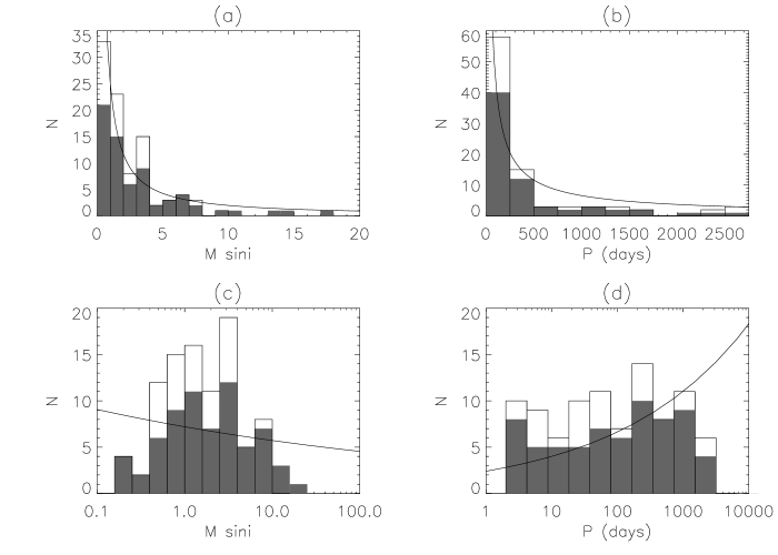
Figure 5: The minimum mass (left panels) and period (right panels) distributions, on linear (top) and logarithmic (bottom) scales. The gray histograms represent all objects, including those with $M\sin i>10M_{\mathrm{J}}$, found in the radial-velocity surveys in Table 1 (67 objects). The unshaded histograms include duplicate discoveries of the same object in different surveys, as discussed in §2.1 (94 objects). The curves show the predictions of our best-fit model, given by equations (25)–28) and (33). As discussed in the paper, the histograms are subject to selection effects at small mass and large period, and there is evidence for a cutoff to the mass distribution above $\sim 10M_{\mathrm{J}}$.

Figure 5 shows the minimum-mass and period distributions of all of the substellar companions found in the surveys in Table 1, along with the simple power-law models that we have used to fit these distributions. The effects of the selection effects at small mass and large period, and the evidence for a cutoff above $\sim 10M_{\mathrm{J}}$, are evident in the bottom panels.

We have described a simple maximum-likelihood method that determines the mass and period distributions of extrasolar planets discovered in multiple surveys. Our method determines and accounts for selection effects on velocity amplitude and period from the data themselves, without relying on the nominal survey parameters. Our best-fit model is defined by equations (3) and equations (25)–(28).

We are indebted to W. Cochran, G. Marcy and M. Mayor for communicating some of the details of their surveys that were used in this statistical analysis. We are particularly grateful to David Weinberg for pointing out a normalization error in an early version of this paper. This research was supported in part by NASA grant NAG5-10456, and by a European Space Agency fellowship.

Survey	$K_{\mathrm{S}}$	duration	number of	number of dis-	references
	(m/s)	(yr)	stars observed	covered planets
Coralie	4	2.5	1000	23	Udry et al.  (2001)
Keck	2–5	5	530	22	Vogt et al.  (2000)
Lick	3–10	13	300	17	Cumming et al.  (1999)
Elodie	10	7	320	13	Udry et al.  (2001)
AFOE	10	6	100	7	Nisenson et al.  (1999)
AAT	3	3.5	200	4	Tinney et al.  (2001)
ESO	8–15	8.5	40	2	Endl et al.  (2000)
McDonald	15–20	10	73	2	Cochran et al.  (2000)

Table 1: Characteristics of eight radial-velocity surveys of extrasolar planets: stated velocity precision of the survey ($K_{\mathrm{S}}$), duration of the program, number of stars observed to date, number of planetary companions discovered ($M\sin i<10M_{\mathrm{J}}$), and references for each survey.

Survey	$\alpha$	$\beta$	$C\times 10^{4}$	$P_{\mathrm{max}}$	$K_{\mathrm{D}}$
				(yr)	($\mathrm{m\ s}^{-1}$)
Coralie	$0.16\pm 0.19$	$-0.23\pm 0.13$	$11.5^{+2.7}_{-2.3}$	$2.1+0.2$	$11.1-0.7$
Keck	$0.06\pm 0.19$	$-0.15\pm 0.12$	$18.1^{+4.2}_{-3.7}$	$3.0+0.4$	$10.3-0.9$
Lick	$-0.03\pm 0.23$	$-0.09\pm 0.12$	$22.2^{+5.9}_{-5.0}$	$6.9+1.7$	$12.9-1.5$
Elodie	$0.51^{+0.43}_{-0.41}$	$-0.44^{+0.17}_{-0.18}$	$32.5^{+11.5}_{-9.5}$	$6.3+1.1$	$36.6-1.9$
AFOE	$0.49^{+0.49}_{-0.46}$	$-0.16^{+0.23}_{-0.24}$	$55.9^{+26.7}_{-20.4}$	$3.6+3.3$	$32.7-3.8$
AAT	$1.78^{+1.2}_{-0.96}$	$-1.08^{+0.45}_{-0.53}$	$31.4^{+19.8}_{-14.1}$	$2.0+0.6$	$38.6-2.8$
ESO	$0.98^{+1.18}_{-0.95}$	$-1.31^{+0.65}_{-0.92}$	$4.2^{+15.8}_{-3.9}$	$6.9+2.0$	$12.9-3.5$
McDonald	$2.09^{+1.92}_{-1.34}$	$-2.46^{+1.11}_{-1.64}$	$0.1^{+2.5}_{-0.09}$	$6.9+1.0$	$12.9-1.6$

Table 2: For each survey, best estimates for the exponents $\alpha$ and $\beta$ and the normalizing constant $C$ in equation (3), the maximum detectable period $P_{\mathrm{max}}$ and the velocity precision $K_{\mathrm{D}}$ in $\mathrm{m\ s}^{-1}$. The fiducial mass and period are $M_{0}=1.5M_{\mathrm{J}}$, $P_{0}=80$ d. The errors on $P_{\mathrm{max}}$ and $K_{D}$ are one-sided, since the maximum likelihood is achieved when these parameters equal the largest period and smallest velocity amplitude found in the survey.

Survey	number of pre-	number of dis-	number of predic-	number of discovered
	dicted planets	covered planets	ted brown dwarfs	brown dwarfs
Coralie	$35^{+6}_{-4}$	23	$13^{+7}_{-4}$	1
Keck	$21^{+3}_{-2}$	22	$8^{+4}_{-3}$	1
Lick	$13\pm 2$	17	$6^{+4}_{-2}$	1
Elodie	$9^{+2}_{-1}$	13	$6^{+4}_{-2}$	–
AFOE	$3\pm 0$	7	$2\pm 1$	–
AAT	$4\pm 1$	4	$3\pm 1$	–
ESO	$2\pm 0$	2	$1\pm 0$	–
McDonald	$3^{+1}_{-0}$	2	$1\pm 1$	–

Table 3: Comparison of predicted and observed numbers of companions.

Figure 1: The left panel shows the correlation between the duration of each survey (from Table 1) and the longest period in the sample. Note that Lick, ESO and McDonald programs have all detected the same long-period planet: $\epsilon$ Eridani, which has an inferred orbital period of $P=2502.1$ days. All of the points lie below the dashed line ($x=y$), indicating that a reliable detection requires following the star for more than one orbital period. The right panel shows the correlation between the stated velocity precision of each survey (from Table 1) and the smallest velocity amplitude of any of their detected planets. Almost all of the points lie well above the dashed line, indicating that determining a reliable orbit requires a velocity amplitude that is significantly larger than the stated velocity precision. The exception is the derived limit for McDonald; in this case $K_{D}$ is set by their detection of a planet in the $\epsilon$ Eri system, for which our approximations of a circular orbit and solar-mass star yield an estimate for the velocity amplitude that is 46% too low (see footnote 1).

Figure 2: Contours of constant likelihood for the combination of all eight surveys. The maximum of $L$ is located at the filled circle, $\alpha=0.12\pm 0.10$, $\beta=-0.26\pm 0.06$. The contour levels represent “$n$–$\sigma$” confidence regions, in which the likelihood function is smaller than its maximum value by $\exp(-n^{2}/2)$.

Figure 3: The estimators of the exponents of the mass and period distribution, $\alpha$ and $\beta$, for the combined eight surveys (filled circles) compared with their values for each individual survey. The estimates are approximately consistent given the uncertainties.

Figure 4: The difference of the modified best parameters $\alpha_{m}$ and $\beta_{m}$ (which depend on the threshold widths $\delta_{u}$ and $\delta_{v}$) and the nominal values of $\alpha$ and $\beta$ as quoted in eqs. (25) and (26).

References

- Basri & Marcy (1997) Basri, G., & Marcy, G. W. 1997, in Star Formation Near and Far, AIP Conf. Proc. 393, eds. S. Holt & L. G. Mundy (New York, AIP), 228
- Cochran et al. (2000) Cochran, W. D., Hatzes, A.P., & Paulson, D.B. 2000, in Planetary Systems in the Universe: Observation, Formation and Evolution, IAU Symp. 202, eds. A. Penny, P. Artymowicz, A.-M. Lagrange and S. Russell (ASP Conf. Ser.) in press
- Cumming et al. (1999) Cumming, A., Marcy, G. W., & Butler, R. P. 1999, ApJ, 526, 890
- Endl et al. (2000) Endl, M., Kürster, M., & Els, S. 2000, A&A, 362, 585
- Hayashi (1981) Hayashi, C. 1981, Progr. Theor. Phys. Suppl., 70, 35
- Jorissen et al. (2001) Jorissen, A., Mayor, M., & Udry, S. 2001, submitted to A&A, astro-ph/0105301
- Marcy & Butler (1998) Marcy, G. W., & Butler, R. P. 1998, ARA&A, 36, 57
- Mayor et al. (1998) Mayor, M., Queloz, D., & Udry, S. 1998, in Brown Dwarfs and Extrasolar Planets, ASP Conf. Ser. 134, eds. R. Rebolo, E. L. Martin, & M. R. Zapatero-Osorio (San Francisco: ASP), 140
- Mazeh (1999) Mazeh, T. 1999, Physics Reports, 311, 317
- Mazeh et al. (1998) Mazeh, T., Goldberg, D., & Latham, D. W. 1998, ApJ, 501, L199
- Nisenson et al. (1999) Nisenson, P., Contos, A., Korzennik, S., Noyes, R., & Brown, T. 1999, in Precise Stellar Radial Velocities, ASP Conf. Ser. 185: IAU Colloq. 170, eds. J. B. Hearnshaw and C. D. Scarfe (San Francisco: ASP), 143
- Stepinski & Black (2000) Stepinski, T. F., & Black, D. C. 2000, A&A, 356, 903
- Stepinski & Black (2001) Stepinski, T. F., & Black, D. C. 2001, A&A, 371, 250
- Tinney et al. (2001) Tinney, C. G., Butler, R. P., Marcy, G. W., Jones, H., Penny, A., Vogt, S., Apps, K., Henry, G. W. 2001, ApJ, 551, 507
- Udry et al. (2001) Udry, S., Mayor, M., & Queloz, D. 2001, in Planetary Systems in the Universe: Observation, Formation and Evolution, IAU Symp. 202, eds. A. Penny, P. Artymowicz, A.-M. Lagrange and S. Russell (ASP Conf. Ser.) in press
- Vogt et al. (2000) Vogt, S., Marcy, G., & Butler, R. P. 2000, ApJ, 536, 902
- Zucker & Mazeh (2001) Zucker, S., & Mazeh, T. 2001, submitted to ApJ, astro-ph/0106042