A PERTURBED TRI-POLYTROPIC MODEL OF THE SUN

Abstract

Based on the Solar Standard Model SSM of Bahcall and Pinsonneault (SSM-BP2000) we developed a solar model in hydrostatic equilibrium using three polytropes, each one associated to the nuclear, the radiative and the convective regions of the solar interior. Then, we apply small periodic and adiabatic perturbations on this tri-polytropic model in order to obtain proper frequencies and proper functions which are in the p-modes range of low order $0<l<5$; for $l=2,3$ and $4$ these values agrees with GOLF observational data within a few percent.

1 Introduction

Polytropic models have largely been used in the study of NRO of a gaseous sphere [Cowling,1941; Kopal,1949; Scuflaire,1974; Tassoul,1980].

We have computed the first modes of a tri-polytropic model (TPM) whose indices $n_{1}=1.50$, $n_{2}=3.78$ and $n_{3}=20$ describes the convective, radiative and nuclear zones respectively of the solar interior. We used Cowling’s approximation [Cowling,1941] which reduces the order of the system of differential equations to 2 (instead of 4). The radial part of the perturbation obeys equations (1) and (2) [Ledoux-Walraven,1958]:

$$\frac{dv}{dr} = \left[\frac{L_{l}^{2}}{\sigma^{2}}-1\right]\frac{P^{\frac{2}{{}_{\Gamma_{1}}}}}{\rho}w$$ (1)

$$\frac{dw}{dr} = \frac{1}{r^{2}}\left[\sigma^{2}-N^{2}\right]\frac{\rho}{P^{\frac{2}{\Gamma_{1}}}}v$$ (2)

where

$$v=r^{2}\delta rP^{\frac{1}{\Gamma_{1}}}$$ (3)

$$w=\frac{P^{\prime}}{P^{\frac{1}{\Gamma_{1}}}}$$ (4)

are proper functions, $l$ is the degree of the spherical harmonic, $\Gamma_{1}$ is the adiabatic exponentent equal to $\frac{5}{3}$, $\sigma$ is the angular frequency, $N$ is the Brunt-Väisälä frequency and $L_{l}$ is the Lamb frequency.

The equations (1) and (2) and the boundary conditions lead to a eigenvalue problem with eigenvalue $\sigma^{2}$, which is the problem to be solved.

2 Polytropes

Our unperturbed model consist of a gas of particles with spherical symmetry, selfgravitating, in hydrostatic equilibrium and with its state equation given by:

$$P=K\rho^{\gamma}=K\rho^{1+\frac{1}{n}}$$ (5)

$K$ and $\gamma$ are parameters that depend only on the polytropic index $n$, and the mass and radius of the configuration. The polytrope theory developed by the ends of the XIX century, can be used to know the dynamical structure of a star, within which local quasistatic thermodynamic changes follows a polytropic process, i.e. one in which the specific heat remains constant. This approach can be used in some regions of Sun’s interior. We have used the pressure and the density data from the sophisticated SSM of Bahcall and Pinsonneault to plot $\gamma=\frac{dLnP}{dLn\rho}$ $vs$ $x$ with $x=r/R_{\odot}$. Various regions clearly emerge. Of these regions, the outermost one ($\gamma_{1}=1.677$, i.e. $n_{1}=1.50$) represents the convective zone where heat transport is achieved by adiabatic convection. It’s SSM output in Fig.1 is approximated rather well by a constant straight line indicating a polytropic behavior. The second intermediate zone labeled radiative zone in Fig.1 can be approach by a polytrope $\gamma_{2}=1.264$, i.e. $n_{2}=3.788$. Finally, we have taken an average of $\gamma$ for the innermost regions labeled nuclear zone, so we represent this zone by a polytrope with $\gamma_{3}=1.050$, i.e $n_{3}=20.0$. This three polytropes have been use by Hendry (1993).

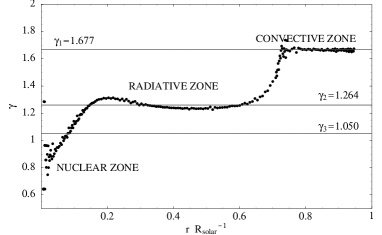
Figure 1: $\gamma$ at the solar interior due to SSM [Bahcall and Pinsonneault,2000]. Regions with $\gamma$ constant are described by polytropic process. The tri-polytropic model is obtained if one assume three values for $\gamma$; $\frac{5}{3}$ in the convective zone, $1.264$ in the radiative zone and $1.050$ in the nuclear zone.

2.1 Three polytropes within the Sun

Following Hendry [Hendry, 1993] we use $\xi$, $\theta$ as the variables in the Lane-Emden equation for the convective zone with index $n_{1}$; $\eta$, $\phi$ as the variables for the radiative zone with index $n_{2}$ and $\zeta$, $\psi$ as the variables for the nuclear zone with index $n_{3}$. Hence the parametric polytropes are:

$$P = K_{1}\rho^{\frac{5}{3}},\textrm{ with }\rho=\lambda_{1}\theta(\xi)^{1.5}$$ (6)

$$P = K_{2}\rho^{1.26},\textrm{ with }\rho=\lambda_{2}\phi(\eta)^{3.85}$$ (7)

$$P = K_{3}\rho^{1.05},\textrm{ with }\rho=\lambda_{3}\psi(\zeta)^{20}$$ (8)

The main challenge is to learn how to fit these three polytropes together. Since the physical quantities $P$, $\rho$ and $M$ are continuous across the interfaces (not for example $\theta$ or $\phi$), the variables $U$ and $V$ given by

$$U=\frac{\xi\theta^{n}}{-\theta^{\prime}}$$ (9)

$$V=\frac{(n+1)\xi(-\theta^{\prime})}{\theta}$$ (10)

are be very useful [Chandrasekhar,1939].

Figure 2: Solutions of the Lane-Emden equation. The center of the Sun as at $V=0$, $U=3$ and its surface at $U=0$, $V=\infty$. We choose $\theta^{\prime}_{\xi_{1}}=-0.00325$ (curve $C$) as a M-Solution for the convective zone and $\phi^{\prime}_{\eta_{1}}=-0.0117$ (curve $E$) as a M-Solution for the radiative zone.

Let us start by considering the convective zone. We take $n_{1}=1.5$ thus $\xi_{1}=3.6538$ and $\theta^{\prime}_{\xi_{1}}=-0.2033$. Though, this polytrope is not being used in the vecinity of $\xi=0$, it is possible to consider all of the solutions of the Lane-Emden equation for $n_{1}=1.50$. These may be generated beginning at $\xi_{1}$ with an arbitrary starting slope and integrating inwards. Solutions with starting slopes less negative than $\theta^{\prime}_{\xi_{1}}$ are of particular interest (in the literature, they are referred to as M-solutions) since these are the ones which intersect the polytrope that represents the radiative zone $n_{2}=3.788$. Four such solutions, translated into the $U$, $V$ variables, are shown in Fig.2, as the curves $A$, $B$, $C$ and $D$ there. Solutions with starting slopes more negative than $\theta^{\prime}_{\xi_{1}}$ (F-solutions) do not intersect the radiative polytrope and so do not need to be considered here. In the same way we have worked the intersection between the nuclear and radiative zones; we have fixed the nuclear polytrope with the $\theta_{20}$ E-solution which intersects the M-solutions (Fig.2, as curves $E$ and $F$) that represents the radiative zone $n_{2}=3.788$, this occur at the neighbors to $0.25R_{\odot}$.

Knowing $\theta(\xi)$, $\phi(\eta)$ and $\psi(\zeta)$ we can deduce the density and pressure curves $\rho(r)$ and $P(r)$. The above model yields a central density of $\rho_{c}=1.483\times 10^{5}$ $Kgm^{-3}$ in comparation with $\rho_{c}=1.299\times 10^{5}$ $Kgm^{-3}$ obtained for the bi-polytropic model BPM [Pinzón-Calvo-Mozo,2001].

A comparison of our BPM and TPM models with the SSM-BP2000 are shown in Fig.3, showing a better fit of the TPM with respect to the SSM-BP2000 in the most central part.

Figure 3: Density (in $g$ $\times$ $cm^{-3}$) at the solar interior for TPM (thin line), for the BPM (dashed line), for the SSM-BP2000 (thick line) and for the $n=3$ one polytrope model.

2.2 Characteristic Frequencies

The characteristic $N$ and $L$ frequencies so called Brunt-Väisälä and Lamb frequencies associated with restoring forces of pressure and gravity in a polytrope of order $n$ can be calculated as functions of radius in terms of the Lane-Emden function $\theta$. Thus, if we define:

$$\omega_{g}=\frac{GM_{\odot}}{R_{\odot}^{3}}$$ (11)

where $R_{\odot}$ and $M_{\odot}$ are the sun mass and the sun radius, and $G$ is the gravitational constant, we can write a normalized Brunt-Väisälä frequency as:

$$N_{n}^{2}\equiv\frac{N^{2}}{\omega_{g}}=\frac{(n-n_{0})}{(n_{0}+1)}\times CC\times\frac{3}{\theta}(\frac{d\theta}{d\xi})^{2}$$ (12)

where $CC$ is the central condensation of the polytrope, defined as the ratio of central density to mean density. The parameter $n_{0}$ is the effective polytropic index associated to the pulsations [Mullan-Ulrich,1988], which in turns related to the adiabatic exponent $\Gamma$ by:

$$\Gamma=1+\frac{1}{n_{0}}$$ (13)

Similarly, the value of the Lamb frequency associated to the mode $l$ is given by:

$$L_{ln}\equiv\frac{L_{l}^{2}}{\omega_{g}}=3\times CC\times l(l+1)\times\frac{\theta}{\xi^{2}}\times\frac{n_{0}+1}{n_{0}(n+1)}$$ (14)

where $\xi$ is the Lane-Emden coordinate.

3 NRO in a Tri-polytropic Model (TPM)

Space oscillation properties of the solutions of equations (1) and (2) are related to the signs of the coefficients given by the second members of these equations. Space oscillations are allowed only in the regions where these coefficients have opposite signs. The limits of these regions are defined by

$$\sigma^{2}=\frac{l(l+1)\Gamma_{1}P}{\rho r^{2}}=L_{l}^{2}$$ (15)

$$\sigma^{2}=N^{2}$$ (16)

Figure 4: Propagation Diagram $(l=2)$ for the BPM (thin lines), for the polytropic index $3$ model (thick lines) and for the SSM-BP2000 (dashed lines). The TPM agree exactly to the BPM except near the center; in this region some points for the TPM are shown.

In the $(x,\omega^{2})$ plane, these equations define two curves. In Fig.4 we have plotted $(15)$ and $(16)$ as thin black curves for the BPM. We can see that the Lamb frequency diverges near to the center; conversely, the Brunt-Väisälä runs from zero at the origin and diverges near the surface. This feature is common in all models. The TPM propagation diagram is very similar to BPM except at the nuclear region, where there is a prominent change. We have been denoted p-modes and g-modes the regions of $(x,\omega^{2})$ plane corresponding to the conditions of position and frequency in the star, allowing spatial oscillations. These regions are characterized by the possibility of existence of progressive acoustic waves and progressive gravity waves respectively [Scuflaire,1974]. Thus we shall refer to these regions as the acoustic and the gravity regions. We have also plotted in the same figure the frequencies (horizontal dot lines) for the first p-modes from $p12-mode$ for the TPM. In addition in the same figure, we can see the propagation diagram for the SSM [Bahcall and Pinsonneault,2000].

Figure 5: Behavior of the boundary condition at surface (equation $(25)$) for TPM model as a function of $\sigma$ in $\mu$Hz.

The equations (1) and (2) are very convenient for the analytical discussion, but for the numerical computations we use the more appropriate form:

$$\frac{dy}{dz}=\frac{l+1}{x}\left[-y+\frac{l}{\omega^{2}}z\right]+\frac{x}{\Gamma_{1}}\frac{GM_{\odot}\rho}{R_{\odot}P}\left(\frac{q}{x^{3}}y-z\right)$$ (17)

$$\frac{dz}{dx}=\frac{1}{x}\left[\omega^{2}y-lz\right]+{}R_{\odot}A\left(\frac{q}{x^{3}}y-z\right)$$ (18)

where we have put:

$$\frac{r}{R_{\odot}} = x$$ (19)

$$\frac{m}{M_{\odot}} = q$$ (20)

$$\frac{\delta(r)}{R_{\odot}} = x^{l-1}y$$ (21)

$$\frac{R_{\odot}P\prime}{GM_{\odot}\rho} = x^{l}z$$ (22)

$$\frac{R_{\odot}^{3}\sigma^{2}}{GM_{\odot}} = \omega^{2}$$ (23)

The regularity condition at the centre, first requires that

$$\omega^{2}y-lz=0$$ (24)

and second, the cancellation at the surface of the lagrangian perturbation of the pressure which can be written down as:

$$\frac{q}{x^{3}}y-z=0$$ (25)

In order to determine the solution uniquely, we impose the normalizing condition

$$y=1$$ (26)

Figure 6: Some p-modes for polytropic models. Figures A and B corresponds to $p_{12}$ modes with $\sigma_{n,l}=\sigma_{12,2}=1796.89$ $\mu$$Hz$ and $\sigma_{12,4}=1880.45$ $\mu$$Hz$ respectively for the $n=3$ one polytrope model. C ($\sigma_{12,2}=2059.86$ $\mu$$Hz$), and D($\sigma_{12,4}=2165.79$ $\mu$$Hz$), are the same modes but in BPM, while E ($\sigma_{21,2}=3368.89$ $\mu$$Hz$) and F ($\sigma_{21,5}=3531.43$ $\mu$$Hz$) represents the $p_{21}$ mode for TPM.

at the centre. With a trial value for $\omega^{2}$ we integrate equations (17) and (18), with initial conditions (24) and (26) using Runge-Kutta method, with a step size taken from a paper of Christensen-Dalsgaard, equation $(A.55)$ [Christensen-Dalsgaard and Mullan,1994]. Usually this solution does not satisfy equation (25) and a new integration is performed with another value of $\omega^{2}$. This procedure is repeated until equation (25) is satisfied, using a Newton-Raphson method to improve the value of $\omega^{2}$.

Figure 7: Comparison of GOLF data with those of the TPM (crosses) and the BPM (open circles) models for $l=2,3,4$; sizes of circles and crosses are inversely proportional to $l$. The Relative Error value is given by $\frac{\sigma_{MODEL}-\sigma_{GOLF}}{\sigma_{GOLF}}\times 100\%$

3.1 Phase Diagram

The radial displacement $\delta(r)$ and the pressure perturbation $P^{\prime}$ are periodic space functions; the variables $v(r)$ and $w(r)$ vary strongly from the center to the surface, then it is impossible to plot them directly along the axes. However, the most appropiate functions:

$$\xi=\pm\log_{10}(1+\left|\frac{\delta(r)}{R_{\odot}}\right|)$$ (27)

$$\zeta=\pm\log_{10}(1+\left|\frac{R_{\odot}P^{\prime}}{GM_{\odot}\rho}\right|)$$ (28)

have been plotted $(27)$ and $(28)$ in each axis of the Fig.6; their signs are chosen according to the signs of the variables $\delta(r)$ and $P^{\prime}$. The number of intersections of each curve with the ordinate axis in Fig.6 (the origin excluded) is equal to the order of the mode. The sense of rotation of this curves is a characteristic feature for the p-modes [Scuflaire,1974].

4 Conclusion

Although we do not use an atmosphere model and the input physics is described by a multi-polytropic structure, the modes obtained from the TPM are close to the observacional data. We show in Fig.7 a comparison with GOLF data, showing an agreement within a few percent (roughly between $4.5\%$ and $7\%$) up to a radial order of $30$. However, we can see that the TPM model is more reliable than the BPM one for all radial orders considered ($n_{r}=10$ to $30$), being noticeable at the higher ones.

References

- (1) Bahcall, M., Pinsonneault, M.:1995, Rev.Mod.Phys, 67, 781 and astro-ph/0010346 (SSM-BP2000)
- (2) Chandrasekhar, S.:1939, An Introduction to the Study of Stellar Structure, Dover Publications, Chicago
- (3) Christensen-Dalsgaard J., Mullan, D.J.:1994, M.N.R.A.S., 270, 921
- (4) Cowling, T.G.:1941, M.N.R.A.S, 101, 367
- (5) Hendry, A.:1993, Am.J.Phys, 61, 10
- (6) Kopal, Z.1949,ApJ, 109,509
- (7) Ledoux, P., Walraven, T.:1958, Handbuch der Physik Vol LI, Springer Verlag, Berlin
- (8) Mullan, D., Ulrich, R.:1988,ApJ, 331, 1013
- (9) Pinzón, G., Calvo Mozo, B.:2001, astro-ph/0102429
- (10) Scuflaire, R.:1974, A&A, 36, 107
- (11) Tassoul, M.:1980,ApJss, 43, 469
- (12) Unno, W., Osaki, Y., Ando, H., Saio, H., Shibahashi, H.:1989, Nonradial Oscillations of Stars, University of Tokio Press, Tokio