Mass ratios of the components in T Tauri binary systems and implications for multiple star formation

Using near-infrared speckle interferometry we have obtained resolved JHK-photometry for the components of 58 young binary systems. From these measurements, combined with other data taken from literature, we derive masses and particularly mass ratios of the components.
We use the J-magnitude as an indicator for the stellar luminosity and assign the optical spectral type of the system to the primary. On the assumption that the components within a binary are coeval we can then place also the secondaries into the HRD and derive masses and mass ratios for both components by comparison with different sets of current theoretical pre-main sequence evolutionary tracks. The resulting distribution of mass ratios is comparatively flat for $M_{2}/M_{1}\geq 0.2$, but depends on assumed evolutionary tracks. The mass ratio is neither correlated with the primary’s mass or the components’ separation. These findings are in line with the assumption that for most multiple systems in T associations the components’ masses are principally determined by fragmentation during formation and not by the following accretion processes.
Only very few unusually red objects were newly found among the detected companions.This finding shows that the observed overabundance of binaries in the Taurus-Auriga association compared to nearby main sequence stars should be real and not the outcome of observational biases related to infrared observing.

1 Introduction

Most stars in the solar neighbourhood are members of multiple systems (e. g. Duquennoy & Mayor Duquennoy91 (1991), Fischer & Marcy Fischer92 (1992)). This raises the question whether most of these systems were formed as binaries or whether they are the result of later capture processes. After high angular resolution techniques in the near infrared (NIR) had been developed at the beginning of the 1990s this problem became an issue of observational astronomy.
A large number of multiplicity surveys in star forming regions (SFRs) and clusters has now been done (see Mathieu et al. Mathieu00 (2000) and references therein). It is still a matter of debate if different environmental conditions of star formation lead to different degrees of multiplicity. One can however conclude that there is at this time no sample of young stars that shows a significant binary deficit compared to nearby main sequence stars. In some SFRs even a strong binary excess is observed. The consequence of these results is that multiplicity must be already established in very early phases of stellar evolution and that star formation to a large extent has to be considered as formation of multiple stars. Multiplicity has to be taken into account if one asks for stellar properties. If this question is addressed to the systems instead of the components, misleading results may be obtained.
In this paper we will discuss young binary systems in the nearby SFRs Taurus-Auriga, Upper Scorpius, Chamaeleon I and Lupus that have been detected by Leinert et al. (Leinert93 (1993)), Ghez et al.  (1997a ) and Köhler et al. (Koehler99 (2000)). We present resolved photometry of the components in the NIR spectral bands J, H and K (Sect. 2). Based on these data we discuss the components in a color-color diagram (Sect. 3) and in a color-magnitude diagram (Sect. 4). Using the J-band magnitude as indicator for the stellar luminosity and pulished spectral types for the primaries, we place the components pairwise into the Hertzsprung-Russell diagram (HRD, Sect. 5) and derive masses and in particular mass ratios from a comparison with theoretical PMS evolutionary models (Sect. 6). Implications of the results for theoretical concepts of multiple star formation and for binary statistics are discussed in Sect. 7.

2 Observational data

2.1 System properties

If not stated otherwise we take the systems’ magnitudes, interstellar extinction coefficients $A_{\mathrm{V}}$ and spectral types from the literature. The references are Kenyon & Hartmann (Kenyon95 (1995)) for Taurus-Auriga, Walter et al. (Walter94 (1994)) and also Köhler et al. (Koehler99 (2000)) for Upper Scorpius, Gauvin & Strom (Gauvin92 (1992)) for Chamaeleon I and Hughes et al. (Hughes94 (1994)) for Lupus. Possible effects of variability are discussed in Sect. 4.2.2.

2.2 Spatially resolved photometry

Data for the objects in Taurus-Auriga were obtained during several observing runs with the NIR camera MAGIC at the 3.5 m-telescope on Calar Alto from 1993 to 1998. Measurements at this telescope before September 1993 were done with a device for one-dimensional speckle-interferometry that has been described by Leinert & Haas (Leinert89 (1989)). Observations of multiple systems in southern SFRs were carried out in May 1998 at the ESO New Technology Telescope (NTT) on La Silla that is also a 3.5 m-telescope, using the SHARP camera of the Max-Planck Institute for Extraterrestrial Physics (Hofmann et al. Hofmann92 (1992)).
Since most binaries of our sample have projected separations of less than $1\arcsec$ a high angular resolution technique is needed to overcome the effects of atmospheric turbulence and to reach the diffraction limit which is $\lambda/D=0\aas@@fstack{\prime\prime}13$ for a 3.5 m-telescope at $\lambda=2.2\,\mu\mathrm{m}$. We have mostly used two-dimensional speckle interferometry. Sequences of typically 1000 images with exposure times of $\approx 0.1\,\mathrm{sec}$ were taken for the object and a nearby reference star. After background subtraction, flatfielding and badpixel correction these data cubes are Fourier-transformed.
We determine the modulus of the complex visibility (i. e. the Fourier transform of the object brightness distribution) from power spectrum analysis. The phase is recursively reconstructed using two different methods: The Knox-Thompson algorithm (Knox & Thompson Knox74 (1974)) and the bispectrum analysis (Lohmann et al. Lohmann83 (1983)). A detailed description of this data reduction process has been given by Köhler et al. (Koehler99 (2000), Appendix A). Modulus and phase show characteristic strip patterns for a binary. In the case of a triple or quadruple star these patterns will be overlayed by similar structures that belong to the additional companion(s).
Fitting a binary model to the complex visibility yields the binary parameters position angle, projected separation and flux ratio. The errors of these parameters are estimated by doing this fit for different subsets of the data. The comparison of our position angles and projected separations with those obtained by other authors that has been done in another paper (Woitas et al. Woitas2001 (2001)) has shown that systematic differences in relative astrometry are negligible. Differences in resolved K-band photometry have an order of magnitude that can be explained by the variability of T Tauri stars.
Together with the system brightness that is taken from the literature in most cases the flux ratio determines the components’ magnitudes. We present the results of our individual measurements in Table 1. To reduce the effect of the variability of T Tauri stars we calculate the mean of all resolved photometric observations in one filter obtained by us and other authors (see caption of Table 2 for references).

2.3 Potential of the data set

Our sample grew out of surveys for multiplicity in star forming regions. With a total of 119 individual components it is of reasonable size. By construction it is largely independent of biases due to duplicity. This makes it well suited for statistical discussions.
From the resolved photometry alone we can check for circumstellar excess emission, search for possible infrared companions, detect contamination by background stars and have some check on whether the components of a binary system are coeval. In the last point we encounter the limitations of our method: the large uncertainty in color, resulting mainly from variability, seriously degrades possible age determinations.
Therefore we use in the HRD known spectral types to derive masses for the components dominating the visual region, and derived masses for the companions on the assumption of coevality. The reliability of these mass determination profits from our explicit knowledge of duplicity.
The presentation of the results starts with those resulting from resolved photometry alone.

3 Color-color diagram

Figure 1: Color-color diagram for the components of weak-lined T Tauri stars (WTTS, left panel) and classical T Tauri stars (CTTS, right panel). The almost vertical solid line denotes the main sequence, with the giant branch to the right (Bessell & Brett BessellBrett88 (1988)). The dotted lines are parallel to the reddening vector (indicated for $A_{\mathrm{V}}=5$ in the lower right of both panels). The cross gives the typical error bars of our observations (see Sect. 4.2). Only in the region labeled ‘A’ and on the main sequence the observed colors are consistent with photospheric emission, whereas for objects located right to this region circumstellar excess emission is present. The numbers in the right panel denote Haro 6-28 B (1), CZ Tau B (2), the infrared companion of XZ Tau (3), the components of FS Tau (4, 5), HN Tau A (6) and the infrared companion of UY Aur (7).

3.1 Presence of circumstellar excess emission

We correct the resolved JHK-photometry for interstellar extinction using the reddening law of Rieke & Lebovsky (Rieke85 (1985)) and applying the $A_{\mathrm{V}}$ given in Table 2 to all components of one system.
The resulting dereddened colors are not necessarily stellar colors, because infrared excess emission caused by circumstellar disks is a common phenomenon in T Tauri stars (e. g. Beckwith et al. Beckwith90 (1990)). For this reason we first consider a subsample of systems that consist of weak-lined T Tauri stars (WTTS). The adopted classification criterion for WTTS is that their H$\alpha$ equivalent width is less than $10\mathrm{{\AA}}$ (Herbig & Bell HBC (1988)). WTTS are not expected to have prominent disks and their mean excess emission in J, H and K is zero (Hartigan et al. Hartigan95 (1995)). Almost all components of these systems have colors comparable to main sequence stars (Fig. 1, left panel) as is expected. The only exceptions are the two components of UX Tau B and the companion of V 773 Tau. For components of systems with classical T Tauri stars (CTTS) where significant circumstellar excess emission is expected, the positions in the color-color diagram are much more spread around(Fig. 1, right panel). These colors cannot be referred to stellar photospheres in a simple way.

3.2 Infrared companion candidates

It is interesting to look for companions with extreme red colors, because these can be candidates for infrared companions (IRCs). IRCs are objects that are very weak or have even not been detected at optical wavelengths, but dominate the system’s brightness in the infrared. They are somewhat puzzling for star formation theory, because some of them appear to be more massive than the optical “primary” but are at the same time more embedded and less evolved.
At this time 8 IRCs are known (Koresko et al. Koresko97 (1997), Ressler & Barsony Ressler01 (2001)). Two of these objects – XZ Tau B and UY Aur B – do indeed show unusual red colors in the color-color diagram (Fig. 1, right panel). Two other known IRCs that belong to our sample – T Tau B and Haro 6-10 B – are not discussed here, because we could not detect those objects in the J-band. In Fig. 1 we have also indicated CZ Tau B, Haro 6-28 B, both components of FS Tau and HN Tau A as unsually red objects. For these systems additional spatially resolved observations at longer and shorter wavelengths will be necessary to decide if they really contain IRCs.
The best candidate for a new IRC is the companion of FV Tau /c that we have observed in H and K, but failed to detect in the J-band. Ghez et al. (1997a ) have proposed HBC 603 B and VW Cha C to be IRCs, because these objects were found by their K-band survey, but missed at $\lambda=0.9\,\mu\mathrm{m}$ by Reipurth & Zinnecker (Reipurth93 (1993)). We have observed these systems in J and H and did not detect any companion either, which calls for additional observations at longer wavelengths.
Extinction by circumstellar envelopes or edge-on disks is not the only possible explanation for extremely red colors. The objects mentioned in this section may also have a very late spectral type and may even be young brown dwarfs. We will discuss the topic of possible substellar companions in Sect. 6.1.
In any case extremely red objects are not frequent among the companions detected by Leinert et al. Leinert93 (1993) in Taurus-Auriga. This indicates that the observed overabundance of binaries in this SFR compared to nearby main sequence stars is real and not the result of using infrared wavelengths for multiplicity surveys among young stars.

4 Color-magnitude diagram

4.1 Conversion of PMS models into the observational plane

For comparison with the data, we convert luminosity $L$ and $T_{\mathrm{eff}}$ for distinct masses and ages from the theoretical atmosphere models to near-infrared colors and magnitudes. To this purpose we use relationships that give the bolometric correction $BC_{\mathrm{V}}$ and several colors as a function of spectral type or the corresponding $T_{\mathrm{eff}}$. These relations are tabulated by Bessell (Bessell91 (1991)), Bessell & Brett (BessellBrett88 (1988)) and Schmidt-Kaler (SchmidtKaler82 (1982)). To interpolate between the datapoints given in these tables we use polynomial fits that have been done by Meyer (Meyer96 (1996)). The apparent J-band magnitude is derived from $L$ and $T_{\mathrm{eff}}$ using the following equation:

$$J = 4.74-2.5\log\left(\frac{L}{L_{\odot}}\right)-BC_{\mathrm{V}}(T_{\mathrm{eff}})-(V-J)_{T_{\mathrm{eff}}}$$

$$+(m-M)-0.282A_{\mathrm{V}}.$$

The coefficient before $A_{\mathrm{V}}$ is taken from the interstellar reddening law of Rieke & Lebovsky (Rieke85 (1985)). For the H- and K-band magnitudes there are similar relations.

4.2 Errors of colors and magnitudes

The magnitude errors that are given in Table 2 are the errors of the mean magnitude that result from averaging over all spatially resolved measurements in a given spectral band. If only one observation has been done the error is calculated from the uncertainties of measured system photometry and flux ratio, as given in Table 1. For the comparison of colors and magnitudes to theoretical PMS models additional error sources have to be taken into account.

4.2.1 Distance

To obtain the distance modulus $m-M$ used in Eq. 4.1 we adopt distances to the SFRs that are the mean of all Hipparcos distances derived for members of the respective association. The values and references are given in Table 1. However, distances to individual objects may be different from these mean values. To take this into account we assume that the radial diameters of the SFRs are as large as their projected diameters on the sky. The latter quantity can be estimated to be $\approx 20^{\circ}$ for Taurus-Auriga (see Fig. 1 in Köhler & Leinert Koehler98 (1998)) as well as for Scorpius-Centaurus (see Fig. 1 in Köhler et al. Koehler99 (2000)). Concerning the mean distances from Table 1 this corresponds to a diameter of 50 pc. We assume here $\pm 25\,\mathrm{pc}$ as uncertainty for the distance of an individual system which is a very conservative estimate: more than two thirds of the stars will be within $\pm$ 15 pc for an even spatial distribution.

Table 1: Adopted distances to stars in nearby SFRs

SFR	distance [pc]	reference
Taurus-Auriga	142 $\pm$ 14	Wichmann et al. (Wichmann98 (1998))
Upper Scorpius	145 $\pm$ 2	de Zeeuw et al. (deZeeuw99 (1999))
Chamaeleon I	160 $\pm$ 17	Wichmann et al. (Wichmann98 (1998))
Lupus	190 $\pm$ 27	Wichmann et al. (Wichmann98 (1998))

Figure 2: Distribution of variability amplitudes for components of young binary systems in the NIR spectral bands J, H and K. They contain all of the systems discussed in this paper for which repeated spatially resolved observations in one filter exist (see Table 1 for our observations and caption of Table 2 for references to other published data).

4.2.2 Variability

T Tauri stars are variable. Although this effect is much less in the infrared compared to optical wavelengths (Nurmanova Nurmanova83 (1983)), it cannot be neglected. We use those components for which there are observations in the same filter at different epochs to estimate the influence of variability on the magnitudes. The distribution of variability amplitudes is given in Fig. 2. The mean amplitudes that we consider as variability errors are $\sigma_{\mathrm{J}}=0.12\,\mathrm{mag}$, $\sigma_{\mathrm{H}}=0.07\,\mathrm{mag}$ and $\sigma_{\mathrm{K}}=0.09\,\mathrm{mag}$. These variations, as derived from our data set, are similar to those in the tabulation of Rydgren et al. (Rydgren84 (1984)) but smaller than those found by Skrutskie et al. (Skrutskie96 (1996)). Therefore our estimate of variability may be somewhat optimistic.

4.2.3 Dereddening

Kenyon & Hartmann (Kenyon95 (1995)) have given for the extinction an error of $\sigma(A_{\mathrm{V}})=0.3\,\mathrm{mag}$ for the systems in Taurus-Auriga. We adopt this error also for the systems in other SFRs.

Figure 3: Components of young binary systems placed into a NIR color-magnitude diagram together with the theoretical PMS model by D’Antona & Mazzitelli (dm98 (1998)). The solid lines are evolutionary tracks for different stellar masses (0.9 to 0.017 $M_{\sun}$), the dashed lines are isochrones for ages from $7\times 10^{4}\,\mathrm{yr}$ to $10^{8}\,\mathrm{yr}$. The latter age is assigned to the main sequence (MS). The crosses denote typical error bars for the stars’ positions, the arrows are reddening vectors for $A_{\mathrm{V}}=5\,\mathrm{mag}$. CTTS are represented by triangles and WTTS by squares. The WTTS indicated with numbers are V 773 Tau A and B (1, 2) and UX Tau A, B and b (3, 4, 5)

4.2.4 Theoretical Atmosphere Models

The following two error sources do not affect colors or magnitudes, but the transformation of theoretical PMS models to observable quantities. By this way they also enter the error discussion:

• For the bolometric correction used in Eq. 4.1 an error $\sigma(BC_{\mathrm{V}})=0.04\,\mathrm{mag}$ is adopted as given by Hartigan et al. (Hartigan94 (1994)).

• As already mentioned in Sect. 4.1 the conversion of luminosity and $T_{\mathrm{eff}}$ into NIR magnitudes and colors uses polynomial fits to tabulated data. This causes an error of $0.07\,\mathrm{mag}$ in J, H and K, except for the models of Baraffe et al (Baraffe98 (1998)), which directly give integrated magnitudes over the near-infrared bands.

4.2.5 Error of colors

All mentioned errors added in quadrature give the uncertainty of a NIR magnitude that has to be considered when placing the components into a color-magnitude diagram. If a color is derived from these magnitudes some errors cancel: The distance is the same for all components and variability is supposed to be negligible if observations at both wavelenghts are carried out in the same night. Unfortunately this is not the case for most of our objects. To obtain a color from $T_{\mathrm{eff}}$ one does not need a bolometric correction, so also the respective error can be discarded.

Figure 4: Examples of colour-magnitude diagrams for two WTTS systems. Left: V819 Tau, the putative companion appears to be a background object. Right: HBC 351: an example for coevality of the components. The data are overplotted with the PMS model by D’Antona & Mazzitelli (dm98 (1998)). The dashed lines denote evolutionary tracks for masses from 0.02 to $0.9\,M_{\sun}$, the solid lines are isochrones for ages $7\cdot 10^{4}$, $10^{5}$, $2\cdot 10^{5}$, $3\cdot 10^{5}$, $5\cdot 10^{5}$, $7\cdot 10^{5}$, $10^{6}$, $2\cdot 10^{6}$, $3\cdot 10^{6}$, $5\cdot 10^{6}$, $7\cdot 10^{6}$, $10^{7}$, $2\cdot 10^{7}$, $3\cdot 10^{7}$, $5\cdot 10^{7}$ and $10^{8}\,\mathrm{yr}$ (MS). The full figure with all 17 colour-magnitude-diagrams is available at CDS as Figure B.1.

4.3 Placing the components into color-magnitude diagrams

In Fig. 3 the placement of the components into a J/(H - K) color-magnitude diagrams is shown. The PMS evolutionary model by D’Antona & Mazzitelli (dm98 (1998)) is also indicated in the Figure. The distribution of objects in a J/(J - K) colour-magnitude diagram would look quite similar.
Almost all components are above the lower main sequence as they are expected to be. But many stars lie in a region that is not covered by the evolutionary tracks. This cannot be corrected by further dereddening, but must be due to the presence of circumstellar color excesses that we have already mentioned above. E.g., nearly all stars that have an unusually large H - K are CTTS (represented by triangles) and the only WTTS in this region are the components of V 773 Tau and UX Tau where we have noticed excess emission already in Sect. 3.1.

4.4 Relative ages of components

Since there is no resolved spectroscopy of the components, we cannot correct for the color excesses mentioned in the previous section. For this reason we restrict the discussion of the components in the color-magnitude diagram to a subsample of 17 systems that consist of WTTS where no significant circumstellar excess emission is expected.

The placement of the individual components into a J/(J-K) color-magnitude diagram is shown in Fig. 4. Object by object, the positons of the components in these plots are compared to the PMS evolutionary model by D’Antona & Mazzitelli (dm98 (1998)) to check for coevality and validity of the association. We have also used the sets of PMS tracks and isochrones given by Swenson et al. (Swenson94 (1994)) and Baraffe et al. (Baraffe98 (1998)) and have obtained similar results.
With respect to the D’Antona & Mazzitelli (dm98 (1998)) tracks in 14 out of 17 cases the components appear to be coeval. Unfortunately, this finding has not much weight because of the large errors in color. Nevertheless some useful checks can be performed. The three problematic cases are V 773 Tau, UX Tau and V 819 Tau. For the first two systems we have already noticed the presence of excess emission (Sect. 3.1 and 4.3). Duchêne et al. (1999b ) have proposed to reclassify UX Tau as a CTTS, because its H$\alpha$ equivalent width is $9.5\,\mathrm{{\AA}}$ and thus above the upper limit for WTTS with spectral type K that is $5\,\mathrm{{\AA}}$ according to Martín (Martin98 (1998)). The companion of V 819 Tau lies far below the main sequence in the color-magnitude diagram. This indicates that V 819 Tau B is in fact not a binary companion, but a chance projected background star.
For HBC 352/353 Fig. 10 yields an age range of about 2$\times$10⁷ - 2$\times$10⁸ yr which is problematic because this age is larger than the age spread found for the Taurus SFR (e. g. Kenyon & Hartmann Kenyon95 (1995)). Also, Martín et al. (Martin94 (1994)) called into question that these are young stars because they do not show significant Lithium line absorption.
With the mentioned exceptions, our data are compatible with the assumption that the components of the T Tauri binaries are coeveal. There are other studies that better prove that this assumption is valid: Brandner & Zinnecker (Brandner97 (1997)) have obtained spatially resolved spectroscopy for the components of eight young binary systems and placed them into the HRD. In all cases the components are coeval. Particularly well this has been shown in the case of the quadruple system GG Tau (White et al. White99 (1999)) from resolved spectroscopy with the HST Faint Object Spectrograph. Below we will use the assumption of coevality to estimate masses for the companions and mass ratios for the components in binary systems.

5 Placing the components into the HRD

In this section we will place the components of young binary systems into the HRD and compare their positions in this diagram with theoretical PMS evolutionary models to derive masses and mass ratios. For this purpose one has to know their luminosities and spectral types. Since these quantities are not known as directly measured values we have to make some assumptions to estimate them from our resolved NIR photometry and the system properties that are given in the literature.

5.1 Luminosities

As described in Sect. 4.1 for the colour-magnitude diagrams, we transform the theoretical atmosphere models that give $T_{\mathrm{eff}}$ and $L$ as functions of mass and age into a diagram in which the luminosity is represented by a NIR magnitude.
Circumstellar excess emission is minimal around $\lambda\approx 1\mu\mathrm{m}$ (e. g. Kenyon & Hartmann Kenyon95 (1995)). For this reason we prefer the J-band magnitudes of the components to H and K as luminosity indicator. It is however not clear if this excess emission is negligible in the J-band. Hartigan et al. (Hartigan95 (1995)) have measured the veiling in optical spectra of T Tauri stars. Assuming that the excess emission in the J-band is $r_{\mathrm{J}}=0.1\times r_{\mathrm{V}}$, where $r_{\lambda}=F_{\lambda,\mathrm{excess}}/F_{\lambda,\ast}$, they come to the conclusion that for a sample of 19 CTTS and 10 WTTS the mean value is consistent with $<r_{\mathrm{J}}>=0.0$. Folha & Emerson (Folha99 (1999)) determined the NIR excess emission directly using infrared spectra of 50 T Tauri stars. Their result is that $<r_{\mathrm{J}}>=0.57$ for the CTTS in their sample and thus much larger than expected. To take this into account we apply an excess correction of $0.49\,\mathrm{mag}$ corresponding to this $<r_{\mathrm{J}}>$, if we use J magnitudes as an indicator for CTTS stellar luminosities. For the WTTS in their sample Folha & Emerson (Folha99 (1999)) find values of $r_{\mathrm{J}}$ that are compatible with zero, so for the components of WTTS systems no excess correction is necessary.

5.2 Spectral types

Figure 5: The components of the young binary system IK Lup placed into the HRD as an example for the method described in Sect. 5. The cross gives the position of the primary, the horizontal dashed lines the locus for the secondary and the respective error. The theoretical model is by Baraffe et al. (Baraffe98 (1998)). The evolutionary tracks are given for masses of 0.04, 0.06, 0.08, 0.10, 0.15, 0.20, 0.25, 0.30, 0.40, 0.50, 0.60, 0.70, 0.80, 0.90, 1.00 and 1.20 $M_{\odot}$, the isochrones denote ages of 1, 2, 5, 10, 20, 50 and 90 Myr. If the components are coeval their masses will be $0.9\pm 0.2\,M_{\odot}$ and $0.3\pm 0.1\,M_{\odot}$.

For nearly all of the systems discussed here we know the combined optical spectral type from the literature (see Sect. 2.1 and Table 2). We assume that these combined spectra represent to a good approximation those of the optical primary components, and we assign the optical spectral type of the system to the brightest component in the J-band. The spectral type and effective temperature of the companion is estimated using the assumption that all components within a system are coeval. We are now ready to place the components into the HRD. The procedure is shown in Fig. 5 using the T Tauri binary system IK Lup as an example. For 48 more systems the placement of the components into the HRD is shown in Fig. 2, available at CDS. The theoretical PMS evolutionary model used is by Baraffe et al. (Baraffe98 (1998)). The position of the primary is determined by its J-band magnitude and the system’s spectral type. For the latter quantity we assume an error of one spectral subclass as given by Kenyon & Hartmann (Kenyon95 (1995)) for the systems in Taurus-Auriga. The companion’s J-band magnitude and the respective error define a locus for the companion in the HRD. If we assume that both components are coeval the companion is situated at the point of intersection between this locus and the isochrone of the primary. In the same way we also defined the loci of the components in the HRD for the evolutionary tracks of Swenson et al. (Swenson94 (1994)) and D’Antona & Mazzitelli (dm98 (1998)).

6 Masses and mass ratios

The procedure described in the previous section yields the components’ masses. For instance, in the IK Lup system (Fig. 5) the components have masses of $0.9\,M_{\odot}$ and $0.3\,M_{\odot}$ with respect to the Baraffe et al. (Baraffe98 (1998)) tracks. The resulting masses derived for the components from all three sets of PMS tracks used are given in Table 2. For some systems (indicated with question marks in Table 2) the primary is located in a region of the HRD that is not covered by the respective tracks. The Swenson et al. (Swenson94 (1994)) model does only cover a mass range above $0.15\,M_{\odot}$, so for some secondaries only upper mass limits can be derived from that model. The errors given in Table 2 reflect the range of tracks that is covered by the stars’ locations in the HRD. These uncertainties are 20 - 30% for most stars and thus quite large. However, all error sources discussed so far are random and not systematic. Therefore in a statistical analysis of these masses that we will do in Sects. 6.2 and 6.3, these uncertainties will partially cancel and have less influence to the results.
There are however additional uncertainties within the PMS models theirselves. One can see from Table 2 that there are discrepancies in masses obtained for the same stars from different PMS models that can be much larger than the indicated errors which trace the uncertainty of our measurements. The components’ mass functions derived from the three models (see Fig. 6) are different at a 99% confidence level which indicates that these mass differences are systematic.
There is now some evidence that the Baraffe et al. (Baraffe98 (1998)) tracks could be preferrable among the current PMS models: White et al. (White99 (1999)) have placed the four components of GG Tau into the HRD and compared their positions with different sets of PMS tracks. They found that the Baraffe et al. (Baraffe98 (1998)) model is best consistent with the assumption that all components are coeval. Simon et al. (Simon2000 (2000)) and Steffen et al. (Steffen2000 (2000)) presented first results of empirical mass determinations from orbital motion around T Tauri stars that are also comparable with the predictions of the Baraffe et al. (Baraffe98 (1998)) model. It would however be premature to consider these results as a final solution of the problem of inconsistent PMS models, mainly because the mentioned observations do not cover the whole range of masses and ages expected for T Tauri stars. Therefore in this paper we will – as we have already done in Sect. 4.4 – rely on the three PMS models given by D’Antona & Mazzitelli (dm98 (1998)), Swenson et al. (Swenson94 (1994)) and Baraffe et al. (Baraffe98 (1998)) and compare the respective results. It can be seen that the uncertainties inherent in the evolutionary model predictions often surpass the uncertainties resulting from the measurement errors.

Table 2: Masses of the components in young binary systems. They are derived placing the components into the HRD as described in Sect. 5 and comparing to the PMS evolutionary tracks from D’Antona & Mazzitelli (dm98 (1998)), Swenson et al. (Swenson94 (1994)) and Baraffe et al. (Baraffe98 (1998)). Question marks indicate that for these systems the primary’s location in the HRD could not be reliably compared to the PMS tracks, because this position falls in a region not covered by the respective tracks.

System	$M_{1}[M_{\sun}]$	$M_{2}[M_{\sun}]$	$M_{1}[M_{\sun}]$	$M_{2}[M_{\sun}]$	$M_{1}[M_{\sun}]$	$M_{2}[M_{\sun}]$
	DM98		Swenson		Baraffe
HBC 351	0.85 $\pm$ 0.1	0.25 $\pm$ 0.1	1.0 $\pm$ 0.1	0.4 $\pm$ 0.1	1.0 $\pm$ 0.1	0.4 $\pm$ 0.1
HBC 352/353	1.0 $\pm$ 0.05	0.9 $\pm$ 0.05	?	?	?	?
HBC 358 Aa	0.35 $\pm$ 0.1	0.35 $\pm$ 0.1	0.7 $\pm$ 0.05	0.7 $\pm$ 0.05	0.4 $\pm$ 0.1	0.4 $\pm$ 0.1
HBC 358 B	0.4 $\pm$ 0.1		0.7 $\pm$ 0.05		0.5 $\pm$ 0.1
HBC 360/361	0.2 $\pm$ 0.05	0.2 $\pm$ 0.05	0.5 $\pm$ 0.1	0.5 $\pm$ 0.1	0.3 $\pm$ 0.1	0.3 $\pm$ 0.1
FO Tau	0.35 $\pm$ 0.05	0.14 $\pm$ 0.04	0.5 $\pm$ 0.1	0.35 $\pm$ 0.1	0.6 $\pm$ 0.1	0.3 $\pm$ 0.1
DD Tau	0.5 $\pm$ 0.1	0.4 $\pm$ 0.1	0.7 $\pm$ 0.1	0.65 $\pm$ 0.1	0.7 $\pm$ 0.1	0.6 $\pm$ 0.1
CZ Tau	0.4 $\pm$ 0.1	0.04 $\pm$ 0.04	0.7 $\pm$ 0.1	$<0.15$	0.6 $\pm$ 0.1	0.10 $\pm$ 0.05
FQ Tau	0.4 $\pm$ 0.05	0.4 $\pm$ 0.05	0.7 $\pm$ 0.05	0.7 $\pm$ 0.05	0.5 $\pm$ 0.1	0.5 $\pm$ 0.1
V 819 Tau	0.45 $\pm$ 0.05	0.04 $\pm$ 0.04	0.7 $\pm$ 0.05	$<0.15$	1.1 $\pm$ 0.1	0.08 $\pm$ 0.02
LkCa 7	0.5 $\pm$ 0.1	0.2 $\pm$ 0.05	0.85 $\pm$ 0.15	0.45 $\pm$ 0.1	1.1 $\pm$ 0.1	0.6 $\pm$ 0.1
FS Tau	0.5 $\pm$ 0.1	0.12 $\pm$ 0.04	0.75 $\pm$ 0.05	0.15 $\pm$ 0.10	0.7 $\pm$ 0.1	0.2 $\pm$ 0.05
FV Tau	0.65 $\pm$ 0.15	0.35 $\pm$ 0.15	1.15 $\pm$ 0.15	0.7 $\pm$ 0.15	1.3 $\pm$ 0.1	1.0 $\pm$ 0.1
UX Tau AC	1.2 $\pm$ 0.2	0.16 $\pm$ 0.05	1.4 $\pm$ 0.2	0.25 $\pm$ 0.1	1.3 $\pm$ 0.1	0.4 $\pm$ 0.1
UX Tau Bb	0.25 $\pm$ 0.05	0.20 $\pm$ 0.05	0.5 $\pm$ 0.1	0.4 $\pm$ 0.1	0.6 $\pm$ 0.1	0.5 $\pm$ 0.1
FX Tau	0.35 $\pm$ 0.05	0.35 $\pm$ 0.05	0.55 $\pm$ 0.1	0.55 $\pm$ 0.1	0.8 $\pm$ 0.2	0.8 $\pm$ 0.2
DK Tau	0.50 $\pm$ 0.05	0.15 $\pm$ 0.05	0.8 $\pm$ 0.15	0.35 $\pm$ 0.1	1.1 $\pm$ 0.1	0.4 $\pm$ 0.1
LkH$\alpha$ 331	0.16 $\pm$ 0.03	0.12 $\pm$ 0.02	0.4 $\pm$ 0.05	0.15 $\pm$ 0.05	0.20 $\pm$ 0.05	0.15 $\pm$ 0.05
HK Tau	0.5 $\pm$ 0.1	0.04 $\pm$ 0.02	0.6 $\pm$ 0.1	$<0.15$	0.7 $\pm$ 0.1	0.08 $\pm$ 0.02
V 710 Tau	0.4 $\pm$ 0.1	0.35 $\pm$ 0.1	0.55 $\pm$ 0.1	0.45 $\pm$ 0.1	0.65 $\pm$ 0.15	0.5 $\pm$ 0.15
HK Tau G2	0.35 $\pm$ 0.05	0.35 $\pm$ 0.05	0.6 $\pm$ 0.1	0.45 $\pm$ 0.1	0.9 $\pm$ 0.1	0.7 $\pm$ 0.1
GG Tau Aa	0.4 $\pm$ 0.05	0.2 $\pm$ 0.05	0.65 $\pm$ 0.05	0.4 $\pm$ 0.05	0.9 $\pm$ 0.1	0.5 $\pm$ 0.1
GG Tau Bb	0.09 $\pm$ 0.02	0.04 $\pm$ 0.02	$<0.15$	$<0.15$	0.2 $\pm$ 0.05	0.04 $\pm$ 0.02
UZ Tau w	0.20 $\pm$ 0.05	0.18 $\pm$ 0.05	0.45 $\pm$ 0.1	0.35 $\pm$ 0.1	0.35 $\pm$ 0.15	0.30 $\pm$ 0.15
GH Tau	0.35 $\pm$ 0.1	0.35 $\pm$ 0.1	0.55 $\pm$ 0.1	0.55 $\pm$ 0.1	0.6 $\pm$ 0.15	0.5 $\pm$ 0.15
Elias 12	0.4 $\pm$ 0.05	0.3 $\pm$ 0.05	0.7 $\pm$ 0.1	0.35 $\pm$ 0.05	1.2 $\pm$ 0.1	0.9 $\pm$ 0.1
IS Tau	1.1 $\pm$ 0.1	0.4 $\pm$ 0.1	1.05 $\pm$ 0.15	0.7 $\pm$ 0.1	0.9 $\pm$ 0.1	0.7 $\pm$ 0.1
GK Tau / GI Tau	0.55 $\pm$ 0.1	0.4 $\pm$ 0.1	0.95 $\pm$ 0.2	0.75 $\pm$ 0.2	1.2 $\pm$ 0.1	1.0 $\pm$ 0.1
HN Tau	0.7 $\pm$ 0.1	0.35 $\pm$ 0.1	0.75 $\pm$ 0.1	0.45 $\pm$ 0.1	0.7 $\pm$ 0.1	0.4 $\pm$ 0.1
CoKu Tau 3	0.4 $\pm$ 0.1	0.16 $\pm$ 0.03	0.75 $\pm$ 0.05	0.35 $\pm$ 0.1	0.6 $\pm$ 0.1	0.3 $\pm$ 0.1
HBC 412	0.35 $\pm$ 0.1	0.3 $\pm$ 0.1	0.6 $\pm$ 0.1	0.5 $\pm$ 0.1	0.55 $\pm$ 0.15	0.50 $\pm$ 0.15
Haro 6-28	0.20 $\pm$ 0.05	0.04 $\pm$ 0.04	0.55 $\pm$ 0.1	$<0.15$	0.25 $\pm$ 0.15	0.06 $\pm$ 0.04
VY Tau	0.60 $\pm$ 0.1	0.25 $\pm$ 0.05	0.85 $\pm$ 0.1	0.35 $\pm$ 0.1	0.8 $\pm$ 0.1	0.4 $\pm$ 0.1
IW Tau	0.7 $\pm$ 0.1	0.6 $\pm$ 0.1	0.95 $\pm$ 0.05	0.85 $\pm$ 0.05	0.9 $\pm$ 0.1	0.8 $\pm$ 0.1
LkH$\alpha$ 332 G1	0.4 $\pm$ 0.05	0.18 $\pm$ 0.03	0.55 $\pm$ 0.1	0.35 $\pm$ 0.1	0.8 $\pm$ 0.2	0.4 $\pm$ 0.1
LkH$\alpha$ 332 G2	0.45 $\pm$ 0.05	0.20 $\pm$ 0.05	0.75 $\pm$ 0.1	0.3 $\pm$ 0.05	1.2 $\pm$ 0.1	0.7 $\pm$ 0.1
LkH$\alpha$ 332	0.7 $\pm$ 0.1	0.6 $\pm$ 0.1	0.95 $\pm$ 0.05	0.8 $\pm$ 0.05	1.0 $\pm$ 0.1	0.8 $\pm$ 0.1
Haro 6-37 Aa	0.7 $\pm$ 0.1	0.09 $\pm$ 0.05	1.05 $\pm$ 0.1	0.2 $\pm$ 0.1	1.1 $\pm$ 0.1	0.3 $\pm$ 0.1
Haro 6-37 /c	0.35 $\pm$ 0.1		0.65 $\pm$ 0.1		0.7 $\pm$ 0.1
RW Aur	1.1 $\pm$ 0.1	0.4 $\pm$ 0.1	1.4 $\pm$ 0.1	0.7 $\pm$ 0.1	1.3 $\pm$ 0.1	0.9 $\pm$ 0.1
NTTS 155203-2338	1.7 $\pm$ 0.1	0.7 $\pm$ 0.1	1.85 $\pm$ 0.2	0.9 $\pm$ 0.1	?	?
NTTS 155219-2314	0.16 $\pm$ 0.04	0.09 $\pm$ 0.04	0.375 $\pm$ 0.075	$<0.15$	0.2 $\pm$ 0.05	0.1 $\pm$ 0.05
NTTS 160735-1857	0.20 $\pm$ 0.05	0.16 $\pm$ 0.04	0.35 $\pm$ 0.05	0.3 $\pm$ 0.05	0.4 $\pm$ 0.1	0.3 $\pm$ 0.1
NTTS 160946-1851	1.7 $\pm$ 0.1	0.6 $\pm$ 0.1	1.9 $\pm$ 0.2	0.75 $\pm$ 0.15	?	?
WX Cha	0.5 $\pm$ 0.1	0.1 $\pm$ 0.04	0.75 $\pm$ 0.1	0.15 $\pm$ 0.1	1.0 $\pm$ 0.1	0.35 $\pm$ 0.1
VW Cha AB	0.6 $\pm$ 0.1	0.4 $\pm$ 0.1	1.05 $\pm$ 0.2	0.7 $\pm$ 0.2	?	?
HM Anon	1.3 $\pm$ 0.1	0.7 $\pm$ 0.1	1.35 $\pm$ 0.2	0.85 $\pm$ 0.05	1.2 $\pm$ 0.1	0.9 $\pm$ 0.1
LkH$\alpha$ 332-17	1.75 $\pm$ 0.1	0.3 $\pm$ 0.05	1.9 $\pm$ 0.2	0.45 $\pm$ 0.1	?	?
IK Lup	0.35 $\pm$ 0.1	0.14 $\pm$ 0.04	0.5 $\pm$ 0.15	0.2 $\pm$ 0.1	0.9 $\pm$ 0.2	0.3 $\pm$ 0.1
HT Lup	1.3 $\pm$ 0.4	0.2 $\pm$ 0.15	1.9 $\pm$ 0.5	0.23 $\pm$ 0.1	?	?
HN Lup	0.25 $\pm$ 0.05	0.25 $\pm$ 0.05	0.4 $\pm$ 0.1	0.4 $\pm$ 0.1	0.7 $\pm$ 0.1	0.6 $\pm$ 0.1
HBC 604	0.11 $\pm$ 0.02	0.05 $\pm$ 0.02	0.23 $\pm$ 0.05	$<0.15$	?	?
HO Lup	0.35 $\pm$ 0.05	0.14 $\pm$ 0.02	0.5 $\pm$ 0.1	0.2 $\pm$ 0.1	0.7 $\pm$ 0.1	0.3 $\pm$ 0.1

Table 3: Mass ratios for the binary pairs from Table 2 derived with respect to the sets of PMS evolutionary tracks by D’Antona & Mazzitelli (dm98 (1998)), Swenson et al. (Swenson94 (1994)) and Baraffe et al. (Baraffe98 (1998)).

System	DM98	Swenson	Baraffe	d[arcsec]
HBC 351	0.29 $\pm$ 0.15	0.40 $\pm$ 0.14	0.40 $\pm$ 0.14	0.61 $\pm$ 0.03
HBC 352/353	0.90 $\pm$ 0.10			8.6 $\pm$ 0.8
HBC 358 Aa	1.0 $\pm$ 0.57	1.0 $\pm$ 0.14	1.0 $\pm$ 0.5	0.15
HBC 360/361	1.0 $\pm$ 0.5	1.0 $\pm$ 0.4	1.0 $\pm$ 0.67	7.2 $\pm$ 0.8
FO Tau	0.40 $\pm$ 0.17	0.70 $\pm$ 0.34	0.50 $\pm$ 0.25	0.165 $\pm$ 0.005
DD Tau	0.80 $\pm$ 0.36	0.93 $\pm$ 0.28	0.86 $\pm$ 0.27	0.57 $\pm$ 0.03
CZ Tau	0.10 $\pm$ 0.13	$<0.21$	0.17 $\pm$ 0.11	0.33 $\pm$ 0.01
FQ Tau	1.00 $\pm$ 0.25	1.0 $\pm$ 0.14	1.0 $\pm$ 0.4	0.79 $\pm$ 0.01
V 819 Tau	0.09 $\pm$ 0.10	$<0.21$	0.07 $\pm$ 0.02	10.5 $\pm$ 0.3
LkCa 7	0.40 $\pm$ 0.18	0.53 $\pm$ 0.21	0.55 $\pm$ 0.14	1.05 $\pm$ 0.01
FS Tau	0.24 $\pm$ 0.13	0.20 $\pm$ 0.15	0.29 $\pm$ 0.11	0.265 $\pm$ 0.005
FV Tau	0.54 $\pm$ 0.36	0.61 $\pm$ 0.21	0.77 $\pm$ 0.14	0.72 $\pm$ 0.10
UX Tau AC	0.13 $\pm$ 0.06	0.18 $\pm$ 0.10	0.31 $\pm$ 0.10	2.7 $\pm$ 0.1
UX Tau Bb	0.80 $\pm$ 0.36	0.80 $\pm$ 0.36	0.83 $\pm$ 0.31	0.138
FX Tau	1.00 $\pm$ 0.29	1.00 $\pm$ 0.36	1.00 $\pm$ 0.50	0.91 $\pm$ 0.01
DK Tau	0.30 $\pm$ 0.13	0.44 $\pm$ 0.21	0.36 $\pm$ 0.13	2.8 $\pm$ 0.3
LkH$\alpha$ 331	0.75 $\pm$ 0.27	0.38 $\pm$ 0.17	0.75 $\pm$ 0.44	0.30 $\pm$ 0.01
HK Tau	0.08 $\pm$ 0.06	$<0.25$	0.11 $\pm$ 0.05	2.4 $\pm$ 0.1
V 710 Tau	0.88 $\pm$ 0.47	0.82 $\pm$ 0.33	0.77 $\pm$ 0.41	3.24 $\pm$ 0.10
HK Tau G2	1.00 $\pm$ 0.29	0.75 $\pm$ 0.29	0.78 $\pm$ 0.20	0.18 $\pm$ 0.01
GG Tau Aa	0.50 $\pm$ 0.19	0.62 $\pm$ 0.12	0.56 $\pm$ 0.17	0.26 $\pm$ 0.01
GG Tau Bb	0.44 $\pm$ 0.32		0.20 $\pm$ 0.15	1.4 $\pm$ 0.2
UZ Tau w	0.90 $\pm$ 0.48	0.78 $\pm$ 0.40	0.86 $\pm$ 0.80	0.34 $\pm$ 0.06
GH Tau	1.00 $\pm$ 0.57	1.00 $\pm$ 0.36	0.83 $\pm$ 0.46	0.35 $\pm$ 0.01
Elias 12	0.75 $\pm$ 0.22	0.50 $\pm$ 0.14	0.75 $\pm$ 0.15	0.41 $\pm$ 0.01
IS Tau	0.36 $\pm$ 0.12	0.67 $\pm$ 0.19	0.78 $\pm$ 0.20	0.21 $\pm$ 0.02
GK Tau / GI Tau	0.73 $\pm$ 0.31	0.79 $\pm$ 0.37	0.83 $\pm$ 0.15	12.2 $\pm$ 0.2
HN Tau	0.50 $\pm$ 0.21	0.60 $\pm$ 0.21	0.57 $\pm$ 0.22	3.1 $\pm$ 0.1
CoKu Tau 3	0.40 $\pm$ 0.18	0.47 $\pm$ 0.16	0.50 $\pm$ 0.25	2.04 $\pm$ 0.07
HBC 412	0.86 $\pm$ 0.53	0.83 $\pm$ 0.31	0.91 $\pm$ 0.52	0.70 $\pm$ 0.01
Haro 6-28	0.20 $\pm$ 0.25	$<0.27$	0.24 $\pm$ 0.30	0.66 $\pm$ 0.02
VY Tau	0.42 $\pm$ 0.15	0.41 $\pm$ 0.17	0.50 $\pm$ 0.19	0.66 $\pm$ 0.02
IW Tau	0.86 $\pm$ 0.27	0.89 $\pm$ 0.10	0.89 $\pm$ 0.21	0.27 $\pm$ 0.02
LkH$\alpha$ 332 G1	0.45 $\pm$ 0.13	0.64 $\pm$ 0.30	0.50 $\pm$ 0.25	0.23 $\pm$ 0.02
LkH$\alpha$ 332 G2	0.44 $\pm$ 0.16	0.40 $\pm$ 0.12	0.58 $\pm$ 0.13	0.30 $\pm$ 0.01
LkH$\alpha$ 332	0.86 $\pm$ 0.27	0.84 $\pm$ 0.10	0.80 $\pm$ 0.18	0.33 $\pm$ 0.03
Haro 6-37 Aa	0.13 $\pm$ 0.09	0.19 $\pm$ 0.11	0.27 $\pm$ 0.12	0.331 $\pm$ 0.005
RW Aur	0.36 $\pm$ 0.12	0.50 $\pm$ 0.11	0.69 $\pm$ 0.13	1.50 $\pm$ 0.01
NTTS 155203-2338	0.41 $\pm$ 0.08	0.49 $\pm$ 0.11		0.758 $\pm$ 0.007
NTTS 155219-2314	0.56 $\pm$ 0.39	$<0.40$	0.50 $\pm$ 0.38	1.485 $\pm$ 0.003
NTTS 160735-1857	0.80 $\pm$ 0.40	0.86 $\pm$ 0.27	0.75 $\pm$ 0.44	0.299 $\pm$ 0.003
NTTS 160946-1851	0.35 $\pm$ 0.08	0.39 $\pm$ 0.12		0.203 $\pm$ 0.006
WX Cha	0.20 $\pm$ 0.12	0.20 $\pm$ 0.16	0.35 $\pm$ 0.14	0.79 $\pm$ 0.04
VW Cha AB	0.67 $\pm$ 0.28	0.67 $\pm$ 0.32		0.66 $\pm$ 0.03
HM Anon	0.54 $\pm$ 0.12	0.63 $\pm$ 0.13	0.75 $\pm$ 0.15	0.27 $\pm$ 0.03
LkH$\alpha$ 332-17	0.17 $\pm$ 0.04	0.24 $\pm$ 0.08		5.3 $\pm$ 0.2
IK Lup	0.40 $\pm$ 0.23	0.40 $\pm$ 0.32	0.33 $\pm$ 0.19	6.5 $\pm$ 0.3
HT Lup	0.15 $\pm$ 0.16	0.12 $\pm$ 0.08		2.8 $\pm$ 0.1
HN Lup	1.00 $\pm$ 0.40	1.00 $\pm$ 0.50	0.86 $\pm$ 0.27	0.24 $\pm$ 0.01
HBC 604	0.45 $\pm$ 0.26	$<0.65$		1.99 $\pm$ 0.09
HO Lup	0.40 $\pm$ 0.11	0.40 $\pm$ 0.28	0.43 $\pm$ 0.20	1.49 $\pm$ 0.07

6.1 Candidates for substellar companions

In six of our systems the mass determination from the D’Antona & Mazzitelli (dm98 (1998)) tracks leads to companion masses that are below the hydrogen burning mass limit of $M\approx 0.08\,M_{\odot}$ (see Oppenheimer et al. Oppenheimer00 (2000) and references therein). This is the case for CZ~Tau B, V~819~Tau B, HK~Tau/c, GG~Tau b, Haro~6-28 B and HBC~604 B. With respect to the Swenson et al. (Swenson94 (1994)) model that does not cover the region close above and below the hydrogen burning mass limit all six mentioned objects have masses below $0.15\,M_{\odot}$. The Baraffe et al. (Baraffe98 (1998)) tracks yield masses of $M\leq 0.08\,M_{\odot}$ for V 819 Tau B, HK Tau/c, GG Tau B and Haro 6-28 B. The primary of HBC 604 could not be reliably compared to the Baraffe et al. (Baraffe98 (1998)) tracks, so we cannot give a Baraffe mass for the secondary.
We emphasize that a definitive classification of a companion as a substellar object is not possible on the basis of our data and requires spatially resolved spectra of the components. It has already been mentioned (Sect. 3.2) that based on NIR colors we cannot distinguish between stars with very late spectral types and deeply embedded objects. HK~Tau/c definitely belongs to the latter class of objects, because it has an edge-on seen disk detected by Stapelfeldt et al. (Stapelfeldt98 (1998)). For two of the other mentioned objects, namely the companions of CZ Tau and Haro 6-28, we have detected unusually large NIR color excesses by placing them into a color-color diagram (see Fig. 1) which makes them good candidates for heavily extincted objects.
V 819 Tau B may be a chance projected background star as has been mentioned in Sect. 4.4. The apparent low luminosity would in this case be the result of underestimating its distance.
Substellar companions to young stars probably do exist. GG Tau b has been placed into the HRD based on spatially resolved spectroscopy by White et al. (White99 (1999)). They derived a mass of $0.044\pm 0.006\,M_{\odot}$ which is in line with our mass estimate of $0.04\,M_{\odot}$ for this object derived from the D’Antona & Mazzitelli (dm98 (1998)) and the Baraffe et al. (Baraffe98 (1998)) models. Meyer et al. (Meyer97 (1997)) have estimated a mass of $\approx 0.06\,M_{\odot}$ for the companion of DI~Tau that has been detected by Ghez et al. (Ghez93 (1993)). This system is not within our object list because its projected separation of 0$\aas@@fstack{\prime\prime}$12 is below the diffraction limit of a 3.5 m telescope in the K-band. There are no strong substellar companion candidates among the components covered by our study.

6.2 The mass function for the components in Taurus-Auriga

Among T Tauri stars in the Taurus-Auriga association there is a significant overabundance of binaries compared to main sequence stars in the solar neighbourhood (see Köhler & Leinert Koehler98 (1998) and references therein). If the binary excess detected with lunar occultation observations, speckle interferometry and direct imaging is extrapolated towards the whole range of projected separations one comes to the conclusion that nearly all stars in this SFR belong to multiple systems. It is therefore interesting to derive the components’ mass function for the Taurus-Auriga association, because this should be a better representation of the mass function in this SFR than the systems’ mass function - including unresolved binaries - that has been given by Kenyon & Hartmann (Kenyon95 (1995)).
The mass functions for the components of young multiple systems in Taurus-Auriga for which we have given masses in Table 2 are plotted in Fig. 6 for the three sets of PMS tracks used. We have now to ask to what degree these mass functions can be representative of the whole binary population in this SFR. Our sample is taken from Leinert et al. (Leinert93 (1993)). It is restricted to systems with projected separations from 0$\aas@@fstack{\prime\prime}$13 to 13″and apparent magnitudes $K_{\mathrm{sys}}\leq 9.5\,\mathrm{mag}$. For the first restriction one has to assume that the components’ masses are not a function of their separation. The latter restriction means that we can detect all primaries with $K_{\mathrm{sys}}\leq 10.25\,\mathrm{mag}$ (for a flux ratio $I_{2}/I_{1}=1$) while the secondaries are complete to a magnitude of K = 12 mag. After transforming the theoretical evolutionary model from the HRD to a diagram where the luminosity is indicated by the K-band magnitude (see Sect. 4.1) one can determine which mass range is completely above the K = 10.25 mag brightness limit for ages less than $10^{7}\,\,\mathrm{yr}$. This leads to completeness limits of $M\geq 0.4M_{\odot}$ (D’Antona & Mazzitelli dm98 (1998) tracks), $M\geq 0.5M_{\odot}$ (Baraffe et al. Baraffe98 (1998) tracks) and $M\geq 0.55M_{\odot}$ (Swenson et al. Swenson94 (1994) tracks). The first incomplete bins are indicated with arrows in Fig. 6. It is thus not possible based on our data to answer the question if and where the components’ mass function has a maximum and how it continues into the substellar regime. For this purpose deep imaging surveys for low luminosity young stars and follow up high angular resolution observations will be necessary. Concerning mass ratios, our sample is much less subject to incompleteness.

Figure 6: Mass function for the components of young binary systems in Taurus-Auriga from Table 2 derived using the PMS evolutionary models from D’Antona & Mazzitelli (dm98 (1998)), Swenson et al. (Swenson94 (1994)) and Baraffe et al.  (Baraffe98 (1998)). The bins indicated with arrows and all bins left of them only represent lower limits, because of the incompleteness of our sample (see Sect. 6.2). The objects represented by the shaded bin the upper right panel can also have lower masses than indicated here, because the Swenson et al. (Swenson94 (1994)) model does only cover masses with $M\geq 0.15\,M_{\odot}$.

6.3 Mass ratios

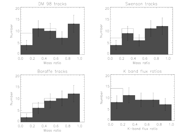
Figure 7: Distribution of mass ratios for the young binary systems from Table 2 derived with respect to three sets of PMS evolutionary models. The open histograms represent all 51 binaries from that table, the shaded histograms show a restricted sample (45 binaries) for which all companions can be detected with the applied observational techniques (see Sect. 6.3). In the lower right panel also the distribution of K band flux ratios is given.

The distribution of mass ratios of binary components and their dependence on other parameters are of special interest, because they can be compared to predictions of theoretical models for multiple star formation (see Sect. 7). To place reliable constraints on this quantity one has to define a complete sample that is unaffected by biases caused by the observational techniques. Köhler et al. (Koehler99 (2000)) have come to the conclusion that using speckle interferometry at a 3.5 m-telescope in the K-band will detect any companion with a projected separation above 0$\aas@@fstack{\prime\prime}$13 and a magnitude difference to the primary of $\Delta K\leq 2.5\,\mathrm{mag}$. The first condition is fulfilled for all components in Table 2. By applying the second restriction and obtaining a homogeneous data set we exclude six systems from the following discussion, namely V 819 Tau, UX Tau AC, HK Tau, HN Tau, WX Cha and LkH$α$ 332-17. They have very faint companions that have been detected using direct imaging.

6.3.1 Mass ratio distribution

The mass ratios derived from three sets of PMS tracks are shown in Table 3. For triple and quadruple systems we have only given them for close pairs in hierarchical systems. The errors indicated in Table 3 are formally derived from the mass errors given in Table 2. This is a conservative estimate, since distance errors affect the components of a binary in a similar way and therefore do not fully influence the mass ratio. To take the uncertainties that are within the PMS models into account we compare the mass ratio distributions derived from the D’Antona & Mazzitelli (dm98 (1998)), Swenson et al. (Swenson94 (1994)) and Baraffe et al (Baraffe98 (1998)) models (Fig. 7). The shaded histograms show the restricted sample, the open histograms represent all pairs from Table 2. The distributions derived from the D’Antona & Mazzitelli (dm98 (1998)) and Swenson et al. (Swenson94 (1994)) tracks are flat for $M_{2}/M_{1}\geq 0.2$ within the uncertainties. The apparent deficit in the first bin is probably due to incomplete detections in this regime. Actually we have found more pairs with mass ratios below $0.2$. The Baraffe et al. (Baraffe98 (1998)) model suggests a rising of the mass ratio distribution towards unity, but this may also be caused by incompletes of the sample at low mass ratios and is not very significant. The distribution for $M_{2}/M_{1}\geq 0.2$ is still compatible with being flat on a 57% confidence level. In discussing the mass ratio distributions given in Fig. 7 one has to take into account that the mean error of the individual mass ratios (Table 3) is about one binsize. This effect will cause a flattening of any given distribution. We will conclude this discussion with the statement that our data does not support the preference of any mass ratios. On the other hand we admit that it would be premature to say that the mass ratio distribution is definetely flat taking into account the large differences between the distributions shown in Fig. 7.
A flat distribution of mass ratios is supported by the distribution of K-band flux ratios (Fig. 7, lower right panel). For low-mass PMS stars there is a K-band mass-luminosity relation of about $L\sim M$ (e. g. Simon et al. Simon92 (1992)), so the distribution of this quantity should in a good approximation resemble that of the mass ratios. There is again no clustering towards $M_{2}/M_{1}=1$. If also the systems with $\Delta K>2.5$, i. e. $F_{2}(K)/F_{1}(K)<0.1$ are included there seems to appear even a slight overabundance of low mass ratios.

Figure 8: Distribution of mass ratios as a function of the projected separation for the three sets of PMS models used in this paper.

Table 4: Dependence of mass ratios with projected separation

	$d_{\mathrm{proj}}<100\,\mathrm{AU}$	$d_{\mathrm{proj}}\geq 100\,\mathrm{AU}$
D’Antona & Mazzitelli (dm98 (1998))
$M_{2}/M_{1}>0.5$	14 $\pm$ 3.7	9 $\pm$ 3.0
$M_{2}/M_{1}\leq 0.5$	12 $\pm$ 3.5	10 $\pm$ 3.2
Swenson et al. (Swenson94 (1994))
$M_{2}/M_{1}>0.5$	16 $\pm$ 4.0	9 $\pm$ 3.0
$M_{2}/M_{1}\leq 0.5$	10 $\pm$ 3.2	8 $\pm$ 2.8
Baraffe et al. (Baraffe98 (1998))
$M_{2}/M_{1}>0.5$	17 $\pm$ 4.1	8 $\pm$ 2.8
$M_{2}/M_{1}\leq 0.5$	8 $\pm$ 2.8	6 $\pm$ 2.5

6.3.2 Correlations between mass ratios and other binary parameters

First, we want to examine a possible correlation of mass ratios and the components’ separations. For this purpose it is useful to convert the measured projected angular separations to physical separations. This allows us to discuss binaries in SFRs with different distances (see Table 1) simultaneously. Moreover this yields a comparison between mass ratios and characteristic length scales like the radii of circumstellar disks. Applying this conversion one has to consider that values for the projected distance obtained with “snap-shot” observations can be very different from the semimajor axis $A$. This cannot be corrected for individual systems. Leinert et al. (Leinert93 (1993)) have however calculated that the relationship between the projected separation $d_{\mathrm{proj}}$ and the semimajor axis $A$ is on average

$$d_{\mathrm{proj}}=0.95\,A.$$ (2)

So for a large sample the distribution of $d_{\mathrm{proj}}$ will resemble the distribution of semimajor axes in a good approximation. In Fig. 8 the mass ratios derived from three sets of PMS evolutionary tracks are plotted as a function of $d_{\mathrm{proj}}$. To present the results more clearly we have divided these scatter plots into four fields (Table 4) and have particularly discriminated between separations that are larger or lower than a typical circumstellar disk radius that is $\approx 100\,\mathrm{AU}$ (e. g. Hartmann Hartmann98 (1998)).
With respect to the D’Antona & Mazzitelli (dm98 (1998)) and the Swenson et al. (Swenson94 (1994)) models in both regions the numbers of systems with low and high mass ratios are comparable within the uncertainties. The result obtained from the Baraffe et al. (Baraffe98 (1998)) model suggests a slight preference of larger mass ratios at lower separations, but this is significant only at the 1$\sigma$ level.

Figure 9: Distribution of mass ratios as function of the primary mass

Table 5: Dependence of mass ratio from primary mass

D’Antona & Mazzitelli (dm98 (1998))
	$M_{1}<0.5\,M_{\odot}$	$M_{1}\geq 0.5\,M_{\odot}$
$M_{2}/M_{1}>0.5$	15 $\pm$ 3.9	8 $\pm$ 2.8
$M_{2}/M_{1}\leq 0.5$	11 $\pm$ 3.3	11 $\pm$ 3.3
Swenson et al. (Swenson94 (1994))
	$M_{1}<0.7\,M_{\odot}$	$M_{1}\geq 0.7\,M_{\odot}$
$M_{2}/M_{1}>0.5$	13 $\pm$ 3.6	11 $\pm$ 3.3
$M_{2}/M_{1}\leq 0.5$	5 $\pm$ 2.2	13 $\pm$ 3.6
Baraffe et al. (Baraffe98 (1998))
	$M_{1}<0.7\,M_{\odot}$	$M_{1}\geq 0.7\,M_{\odot}$
$M_{2}/M_{1}>0.5$	10 $\pm$ 3.2	15 $\pm$ 3.9
$M_{2}/M_{1}\leq 0.5$	6 $\pm$ 2.5	8 $\pm$ 2.8

Finally we ask for a correlation between the mass ratio and the primary mass. The result is shown in Fig. 9 and Table 5. The threshold between “low” and “high” primary masses is arbitrarily chosen to have a comparable number of objects in both groups for each theoretical PMS model considered. With regard to the Baraffe et al. (Baraffe98 (1998)) model the behaviour of both groups is the same. The D’Antona & Mazzitelli (dm98 (1998)) and Swenson et al. (Swenson94 (1994)) models suggest a preference of higher mass ratios for lower primary masses. The latter result has also been mentioned by Leinert et al. (Leinert93 (1993)) on the basis of K band magnitudes and flux ratios.
We conclude that correlations between mass ratio and other binary parameters are weak if they exist at all.

7 Discussion

7.1 Theoretical models for multiple star formation

It is now widely believed that fragmentation during protostellar collapse is the major process for forming multiple stars in low-density SFRs as discussed here (e. g.  Clarke et al. Clarke2000 (2000)). Our results generally are in line with this assumption:

• We have some additional support from our data for coeval formation of the components (Sect. 4.4). Capture processes of independently formed single stars (that would produce a widespread distribution of relative ages) should not play a dominant role in the formation of the binaries discussed here.

• There are only a few companions with masses $M\leavevmode\nobreak\ \leq\leavevmode\nobreak\ 0.1\leavevmode\nobreak\ \,\leavevmode\nobreak\ M_{\odot}$ which is a typical mass of a T Tauri stars’ disk (Beckwith et al.  Beckwith90 (1990)). Furthermore these low mass companions do not preferentially occur at separations $d\leq 100\,\mathrm{AU}$ that are comparable to typical disk radii. This is difficult to reconcile with the idea that a large number of companions is formed from disk instabilities.

• Fragmentation during protostellar collapse does not lead to a preference of distinct mass ratios or to a dependence of mass ratio from other binary parameters like the components’ separation (e. g. Ghez et al. Ghez2000 (2000)). We have indeed not seen any such correlations (Sect. 6.3).

Regarding the last item one has however to consider that there is a large time span between the end of numerical simulations of fragmentation during protostellar collapse and the state of dynamically stable T Tauri multiple systems as observed by us. Particularly, at the end of the simulations presented e. g. by Burkert et al. (Burkert96 (1996)) only $\approx 10\%$ of the parent cloud’s mass has condensed into fragments. Therefore it is a highly important question how subsequent accretion processes influence the properties of young multiple systems. Since it is not possible today to cover the entire evolution of a molecular cloud core into a binary system with one simulation, theory has to take a different approach.
For this purpose Bate (Bate97 (1997), Bate98 (1998)) and Bate & Bonnell (BateBonnell97 (1997)) have simulated the behaviour of a “binary” formed out of two point masses that are situated in a cavity within a surrounding gas sphere. The mass ratio of the binary and the angular momentum of the infalling material are variable initial conditions. The result of these simulations is that in the course of the accretion process the system’s mass ratio increases and approaches unity if the total cloud mass is accreted. Mass ratios close to unity should be more probable in close systems than for wide pairs.
This is not in agreement with our result (Sect. 6.3) that there is no significant preference of mass ratios close to unity and that the mass ratio is probably independent of the components’ separation. So it seems that the initial conditions used by Bate & Bonnell are somehow unrealistic and that the “final” stellar masses are more dependent on the fragment masses than on the following accretion processes. One explanation for this could be that in the course of protobinary evolution most of the initial mass is condensed into fragments, before accretion becomes important. Another idea is that there is some process that halts accretion before a large amount of the remaining cloud mass is accreted onto the fragments. In any case our knowledge about this issue is preliminary and additional theoretical and observational effort is necessary to decide what physical processes determine stellar masses.

7.2 Implications for binary statistics

Multiplicity surveys by Leinert et al. (Leinert93 (1993)) and Ghez et al. (Ghez93 (1993)) led to the surprising result that there is a significant overabundance of binaries in the Taurus-Auriga SFR compared to main sequence stars in the solar neighbourhood. This result was further proved by the follow-up studies done by Simon et al. (Simon95 (1995)) and Köhler & Leinert (Koehler98 (1998)). Although this paper is not directly concerned with binary statistics, we can draw some conclusions that further support the idea that this binary excess is real and not a result of observational biases.
If one compares the binary frequency among young and evolved stars one has to take into account that due to evolutionary effects companions can be relatively bright in their PMS phase, but invisible on the main sequence stage. This is particularly the case for substellar companions. One has further to consider that the multiplicity surveys were done at infrared wavelengths in SFRs, but in the optical range for main sequence stars. So there might be a bias that supports the detection of very red “infrared companions” (IRCs, see Sect. 3.2) in the vicinity of PMS stars. Another problem is that the surveys in Taurus-Auriga and the solar neighbourhood could be not directly comparable if they were sensitive to a different range of mass ratios and thus stellar masses.
If the presence of substellar companions or IRCs in the vicinity of T Tauri stars in Taurus-Auriga were a common phenomenon this could at least partially explain the observed binary excess in this SFR. Our results presented in Sect. 3.2 and 6.1 show that this is not the case: Köhler & Leinert (Koehler98 (1998)) have found that after applying a statistical correction for chance projected background stars there are $48.9\pm 5.3$ companions per 100 primaries (including single stars) in Taurus-Auriga. We have denoted only 5 out of 40 companions (for which we have given masses in Table 2) as candidates for substellar objects based on masses derived from the D’Antona & Mazzitelli (dm98 (1998)) PMS evolutionary tracks (Sect. 6.1). With respect to the Baraffe et al. (Baraffe98 (1998)) model this number is even lower. If we take the mentioned 5 out of 40 companions as an estimate for the real number of brown dwarf companions in Taurus-Auriga and subtract this from the companion frequency given by Köhler & Leinert (Koehler98 (1998)) this value diminishes to $42.8\pm 6.0$. This is still far above the value of $25.3\pm 3.9$ that was given by Duquennoy & Mayor (Duquennoy91 (1991)) for G-dwarfs in the solar neighbourhood. Furthermore we have found that only 3 out of 51 companions in Taurus-Auriga are detectable in the H-band and at longer wavelengths, but were missed at $1.25\,\mu\mathrm{m}$, so IRCs are probably not a frequent phenomenon. The binary frequency does not have to be corrected for IRCs, because their successors in the main sequence phase will be “normal” stellar companions (see Koresko et al. Koresko97 (1997) for estimates of IRCs’ masses).
Duquennoy & Mayor (Duquennoy91 (1991)) have claimed that their sample is complete for mass ratios $M_{2}/M_{1}\geq 0.1$. It has already been mentioned by Köhler & Leinert (Koehler98 (1998), Sect. 5.2) that the completeness limit of the binary surveys in Taurus-Auriga is in any case not lower, the actual value dependent on the mass-luminosity relation used. We can further prove this result, because there are only 2 out of 51 systems with mass ratios less than 0.1 with respect to the D’Antona & Mazzitelli (dm98 (1998)) PMS model and 1 out of 50 considering the Baraffe et al. (Baraffe98 (1998)) tracks (Table 3).
We conclude that the observed binary excess in Taurus-Auriga compared to nearby main sequence stars is neither the result of a higher sensitivity in mass ratio nor a consequence of a large frequency of substellar or infrared companions. The strange overabundance of binaries in Taurus-Auriga remains a fact also after this more detailed analysis of the systems found by Leinert et al. (Leinert93 (1993)).

8 Summary

From speckle interferometry and direct imaging we have derived resolved JHK photometry for the individual components of T Tauri binary systems in nearby star forming regions. These measurements are combined with other data taken from literature (resolved JHK photometry from other authors, system magnitudes and spectral types, extinction coefficients) to study properties of the components in young binary systems. The main results are:

• We have found only very few unusually red objects that may be young substellar objects or infrared companions. Their number is too small to have significantly influenced the binary statistics in Taurus-Auriga.

• The placement of the components into NIR color magnitude diagrams is affected by large errors and thus allows no precise determination of stellar ages from PMS evolutionary models. We can however detect problematic cases and find that V~819~Tau B is probably an unrelated background object. The locations of the components of the 16 other WTTS systems into the the CMDs are in line with the assumption that all components within a system are coeval.

• The determination of masses from the HRD has been performed using the following procedure: We derive stellar luminosities from the J-band magnitudes, assign the optical system spectral type to the primary and use the assumption that all components within one system are coeval.

• The use of three different sets of PMS tracks then yields mass functions that are different at the 99% confidence level. For this reason we discuss the results of all three models used separately. These differences tend to be larger than the uncertainties resulting from observational errors. In addition, the latter mass errors are random and thus partially cancel in a statistical discussion.

• Within the uncertainties the distribution of mass ratios is flat for $M_{2}/M_{1}\geq 0.2$. There are no significant correlations between mass ratio and projected separation or mass ratio and primary mass. These results are in line with the wideley accepted idea that binaries are formed by fragmentation during protostellar collapse processes. Moreover, they suggest that the final masses of the components are largely determined by fragmentation itself and not by subsequent accretion.

Appendix A Near-infrared photometry for the components of young binary systems

The spatially resolved observations of T Tauri binary systems obtained by the authors are listed in Table A1. Column 1 gives the most common name of the object, columns 2 and 3 the wavelength band and the date of observation, column 4 the brightness ratio (secondary/primary, usually but not always $<$ 1), columns 5 through 7 the magnitude of system, primary and secondary components in the respective wavelength band.

Table A2 contains the adopted near-infrared magnitudes of the components of the young binary systems which compose our sample. The values given here are the mean of all spatially resolved photometric observations, i. e. our data from Table 1 and measurements published by Chelli et al. (Chelli95 (1995)), Duchêne (1999a ), Ghez et al. (Ghez93 (1993), 1997a , 1997b ), Haas et al. (Haas90 (1990)), Hartigan et al. (Hartigan94 (1994)), Köhler et al. (Koehler99 (2000)), Moneti & Zinnecker (Moneti91 (1991)), Richichi et al. (Richichi99 (1999)), Roddier et al. (Roddier96 (1996)) and Simon et al. (Simon92 (1992)). The values for visual extinction $A_{\mathrm{V}}$ and the spectral type given with the primaries, belong to the systems (see Sect. 2.1 for references). The numbers in the last column denote the star forming region: Taurus-Auriga (1), Upper Scorpius (2), Chamaeleon I (3) and Lupus (4).

Table 1: Spatially resolved observations of young T Tauri binary systems obtained by the authors.

System	Filter	Date	$I_{2}/I_{1}$	$m_{\mathrm{Sys}}$	$m_{\mathrm{Prim}}$	$m_{\mathrm{Sec}}$
HBC 351	J	30 Sep 1993	0.165 $\pm$ 0.004	9.92 $\pm$ 0.05	10.09 $\pm$ 0.05	12.04 $\pm$ 0.07
	H	8. Jan 1993	0.190 $\pm$ 0.015	9.30 $\pm$ 0.02	9.49 $\pm$ 0.03	11.29 $\pm$ 0.09
	K	16. Feb 1992	0.22 $\pm$ 0.02	9.15	9.37 $\pm$ 0.02	11.01 $\pm$ 0.08
HBC 358 B	J	5. Oct 1993		11.33 $\pm$ 0.06
	H	8. Jan 1993		10.75 $\pm$ 0.06
	K	16. Feb 1992		10.44 $\pm$ 0.09
LkCa 3	J	5. Oct 1993	0.62 $\pm$ 0.02	8.47	8.99 $\pm$ 0.01	9.51 $\pm$ 0.02
	H	27. Sep 1991	0.60 $\pm$ 0.03	7.74 $\pm$ 0.01	8.25 $\pm$ 0.03	8.80 $\pm$ 0.04
		29. Sep 1996	0.885 $\pm$ 0.011		8.43 $\pm$ 0.02	8.56 $\pm$ 0.02
	K	6. Dec 1990	0.5	7.52 $\pm$ 0.05	7.96 $\pm$ 0.05	8.71 $\pm$ 0.05
		19. Nov 1997	0.755 $\pm$ 0.007		8.13 $\pm$ 0.05	8.44 $\pm$ 0.06
V 773 Tau	J	5. Oct 1993	0.113 $\pm$ 0.005	7.65 $\pm$ 0.05	7.77 $\pm$ 0.05	10.13 $\pm$ 0.09
	H	8. Jan 1993	0.15 $\pm$ 0.02	6.85 $\pm$ 0.09	7.00 $\pm$ 0.11	9.06 $\pm$ 0.22
FO Tau	J	7. Oct 1993	0.30 $\pm$ 0.01	9.70 $\pm$ 0.07	9.99 $\pm$ 0.08	11.28 $\pm$ 0.09
		29. Nov 1996	0.55 $\pm$ 0.05		10.18 $\pm$ 0.11	10.83 $\pm$ 0.14
		16. Nov 1997	0.63 $\pm$ 0.02		10.23 $\pm$ 0.08	10.73 $\pm$ 0.09
	H	7. Jan 1993	0.93 $\pm$ 0.03	8.71 $\pm$ 0.05	9.42 $\pm$ 0.07	9.50 $\pm$ 0.07
		16. Nov 1997	0.698 $\pm$ 0.014		9.28 $\pm$ 0.06	9.68 $\pm$ 0.06
	K	19. Sep 1991	0.92 $\pm$ 0.04	8.18 $\pm$ 0.03	8.89 $\pm$ 0.05	8.98 $\pm$ 0.05
		14. Dec 1994	0.72 $\pm$ 0.02		8.76 $\pm$ 0.04	9.13 $\pm$ 0.05
		9. Oct 1995	0.648 $\pm$ 0.018		8.72 $\pm$ 0.04	9.19 $\pm$ 0.05
		27. Sep 1996	0.628 $\pm$ 0.019		8.71 $\pm$ 0.04	9.21 $\pm$ 0.05
DD Tau	J	5. Dec 1990	0.79 $\pm$ 0.01	9.47 $\pm$ 0.04	10.10 $\pm$ 0.05	10.36 $\pm$ 0.05
	H	5. Dec 1990	0.79 $\pm$ 0.01	8.52 $\pm$ 0.07	9.15 $\pm$ 0.08	9.41 $\pm$ 0.08
	K	5. Dec 1990	0.64 $\pm$ 0.01	7.87 $\pm$ 0.07	8.41 $\pm$ 0.08	8.89 $\pm$ 0.08
CZ Tau	J	29. Nov 1996	0.120 $\pm$ 0.005	10.51 $\pm$ 0.12	10.63 $\pm$ 0.12	12.94 $\pm$ 0.16
	H	9. Jan 1993	0.23 $\pm$ 0.01	9.74 $\pm$ 0.03	9.96 $\pm$ 0.04	11.56 $\pm$ 0.07
	K	19. Mar 1992	0.46 $\pm$ 0.03	9.28 $\pm$ 0.03	9.69 $\pm$ 0.05	10.53 $\pm$ 0.08
		28. Sep 1996	0.183 $\pm$ 0.004		9.46 $\pm$ 0.03	11.30 $\pm$ 0.04
FQ Tau	J	16. Nov 1997	1.06 $\pm$ 0.01	10.61 $\pm$ 0.02	11.39 $\pm$ 0.03	11.33 $\pm$ 0.02
	H	27. Sep 1991	1.23	9.90 $\pm$ 0.07	10.77 $\pm$ 0.07	10.55 $\pm$ 0.07
		16. Nov 1997	1.109 $\pm$ 0.016		10.71 $\pm$ 0.08	10.60 $\pm$ 0.08
	K	22. Sep 1991	0.90 $\pm$ 0.01	9.47 $\pm$ 0.31	10.17 $\pm$ 0.32	10.28 $\pm$ 0.32
V 819 Tau	J	2. Oct 1993			9.45 $\pm$ 0.03	12.96 $\pm$ 0.06
	H	2. Oct 1993			8.76 $\pm$ 0.08	12.39 $\pm$ 0.08
LkCa 7	J	5. Oct 1993	0.414 $\pm$ 0.008	9.25	9.63 $\pm$ 0.01	10.58 $\pm$ 0.01
	H	27. Sep 1991	0.44 $\pm$ 0.02	8.58	8.98 $\pm$ 0.02	9.87 $\pm$ 0.03
	K	19. Sep 1991	0.56 $\pm$ 0.02	8.36 $\pm$ 0.03	8.84 $\pm$ 0.04	9.47 $\pm$ 0.05
FS Tau	J	29. Nov 1996	0.188 $\pm$ 0.007	10.66 $\pm$ 0.13	10.85 $\pm$ 0.14	12.66 $\pm$ 0.16
	H	28. Sep 1996	0.183 $\pm$ 0.008	9.14 $\pm$ 0.09	9.32 $\pm$ 0.10	11.17 $\pm$ 0.13
	K	19. Nov 1997	0.138 $\pm$ 0.005	7.74 $\pm$ 0.26	7.88 $\pm$ 0.26	10.03 $\pm$ 0.29
FW Tau	H	27. Sep 1996	0.76 $\pm$ 0.10	9.78	10.39 $\pm$ 0.06	10.69 $\pm$ 0.08
	K	17. Oct 1989	1.00 $\pm$ 0.01	9.37	10.12 $\pm$ 0.01	10.12 $\pm$ 0.01
		13. Dec 1994	0.61 $\pm$ 0.10		9.89 $\pm$ 0.07	10.42 $\pm$ 0.11
		9. Oct 1995	1.00 $\pm$ 0.05		10.12 $\pm$ 0.03	10.12 $\pm$ 0.03
FV Tau	J	1. Sep 1990	0.71 $\pm$ 0.05	9.51 $\pm$ 0.10	10.09 $\pm$ 0.13	10.46 $\pm$ 0.14
		30. Nov 1996	0.38 $\pm$ 0.04		9.86 $\pm$ 0.13	10.91 $\pm$ 0.18
	H	1. Sep 1990	0.68 $\pm$ 0.02	8.22 $\pm$ 0.13	8.78 $\pm$ 0.14	9.20 $\pm$ 0.15
	K	1. Sep 1990	0.83 $\pm$ 0.01	7.37 $\pm$ 0.10	8.03 $\pm$ 0.11	8.23 $\pm$ 0.11
		9. Oct 1995	0.695 $\pm$ 0.007		7.94 $\pm$ 0.10	8.34 $\pm$ 0.11
FV Tau /c	H	9. Jan 1991	0.03	9.42 $\pm$ 0.02	9.45 $\pm$ 0.02	13.26 $\pm$ 0.03
	K	9. Oct 1995	0.076 $\pm$ 0.004	8.80 $\pm$ 0.02	8.88 $\pm$ 0.02	11.68 $\pm$ 0.03
UX Tau AC	J	16. Nov 1997			8.97 $\pm$ 0.09	11.85 $\pm$ 0.09
FX Tau	J	20. Mar 1991	0.93 $\pm$ 0.03	9.16 $\pm$ 0.06	9.87 $\pm$ 0.08	9.95 $\pm$ 0.08
		30. Nov 1996	0.934 $\pm$ 0.004		9.88 $\pm$ 0.06	9.95 $\pm$ 0.06
	H	20. Mar 1991	0.78 $\pm$ 0.01	8.75 $\pm$ 0.14	9.37 $\pm$ 0.15	9.65 $\pm$ 0.15
		16. 11. 1997	0.775 $\pm$ 0.012		9.37 $\pm$ 0.15	9.65 $\pm$ 0.15

Table 1: continued

System	Filter	Date	$I_{2}/I_{1}$	$m_{\mathrm{Sys}}$	$m_{\mathrm{Prim}}$	$m_{\mathrm{Sec}}$
FX Tau	K	4. Dec 1990	0.54 $\pm$ 0.05	8.14 $\pm$ 0.14	8.61 $\pm$ 0.18	9.28 $\pm$ 0.21
		20. Mar 1991	0.56 $\pm$ 0.01		8.63 $\pm$ 0.15	9.25 $\pm$ 0.15
		18. Oct 1991	0.509 $\pm$ 0.001		8.59 $\pm$ 0.14	9.32 $\pm$ 0.14
DK Tau	J	16. Nov 1997			9.15 $\pm$ 0.09	10.52 $\pm$ 0.10
Lk H$\alpha$ 331	J	26. Jan 1994	0.706 $\pm$ 0.023	9.85	10.43 $\pm$ 0.01	10.81 $\pm$ 0.02
	H	6. Jan 1993	0.91 $\pm$ 0.02	8.99	9.69 $\pm$ 0.01	9.79 $\pm$ 0.01
		29. Sep 1996	0.70 $\pm$ 0.01		9.57 $\pm$ 0.01	9.95 $\pm$ 0.01
	K	29, Oct 1991	0.73 $\pm$ 0.04	8.68	9.28 $\pm$ 0.03	9.62 $\pm$ 0.03
		9. Oct 1995	0.66 $\pm$ 0.03		9.23 $\pm$ 0.02	9.68 $\pm$ 0.03
XZ Tau	J	27. Jan 1994	1.51 $\pm$ 0.03	9.91 $\pm$ 0.32	10.91 $\pm$ 0.33	10.46 $\pm$ 0.33
		30. Nov 1996	3.54 $\pm$ 0.31		11.55 $\pm$ 0.39	10.18 $\pm$ 0.34
	K	28. Jan 1994	0.41 $\pm$ 0.01	8.05 $\pm$ 0.56	8.42 $\pm$ 0.57	9.39 $\pm$ 0.58
		22. Nov 1997	0.316 $\pm$ 0.007		8.35 $\pm$ 0.57	9.60 $\pm$ 0.58
HK Tau G2	J	26. Jan 1994	0.764 $\pm$ 0.023	9.41 $\pm$ 0.09	10.03 $\pm$ 0.10	10.32 $\pm$ 0.11
	H	6. Jan 1993	0.69 $\pm$ 0.07	8.44 $\pm$ 0.06	9.01 $\pm$ 0.10	9.41 $\pm$ 0.13
		27. Jan 1994	0.85 $\pm$ 0.12		9.11 $\pm$ 0.13	9.28 $\pm$ 0.14
		27. Sep 1996	0.76 $\pm$ 0.05		9.05 $\pm$ 0.09	9.35 $\pm$ 0.10
	K	28. Sep 1991	0.88 $\pm$ 0.03	8.05 $\pm$ 0.02	8.74 $\pm$ 0.04	8.87 $\pm$ 0.04
		9. Oct 1995	0.85 $\pm$ 0.06		8.72 $\pm$ 0.03	8.89 $\pm$ 0.04
		19. Nov 1997	0.587 $\pm$ 0.017		8.55 $\pm$ 0.03	9.13 $\pm$ 0.04
GG Tau Aa	J	27. Jan 1994	0.543 $\pm$ 0.004	9.01 $\pm$ 0.07	9.48 $\pm$ 0.01	10.14 $\pm$ 0.01
	H	2. Nov 1991	0.549 $\pm$ 0.009	7.83 $\pm$ 0.05	8.31 $\pm$ 0.06	8.96 $\pm$ 0.06
		24. Sep 1994	0.417 $\pm$ 0.017		8.31 $\pm$ 0.05	8.95 $\pm$ 0.06
	K	2. Nov 1990	0.64 $\pm$ 0.01	7.30 $\pm$ 0.03	7.84 $\pm$ 0.04	8.32 $\pm$ 0.04
		21. Oct 1991	0.32 $\pm$ 0.05		7.77 $\pm$ 0.04	8.44 $\pm$ 0.06
		16. Nov 1997	0.564 $\pm$ 0.004		7.79 $\pm$ 0.03	8.41 $\pm$ 0.03
		10. Oct 1998	0.476 $\pm$ 0.005		7.72 $\pm$ 0.03	8.53 $\pm$ 0.04
GG Tau Bb	J	27. Jan 1994			11.44 $\pm$ 0.06	13.12 $\pm$ 0.09
	H	10. Jan 1993			10.26 $\pm$ 0.06	12.58 $\pm$ 0.06
	K	2. Nov 1990			9.99 $\pm$ 0.10	11.79 $\pm$ 0.10
UZ Tau w	J	26. Jan 1994	0.76 $\pm$ 0.07	9.64	10.25 $\pm$ 0.04	10.55 $\pm$ 0.06
	H	9. Jan 1993	0.69 $\pm$ 0.02	8.67	9.24 $\pm$ 0.01	9.64 $\pm$ 0.02
		29. Sep 1996	0.66 $\pm$ 0.02		9.22 $\pm$ 0.01	9.67 $\pm$ 0.02
GH Tau	J	26. Jan 1994	0.89 $\pm$ 0.01	9.22 $\pm$ 0.08	9.91 $\pm$ 0.09	10.04 $\pm$ 0.09
	H	6. Jan 1993	1.30 $\pm$ 0.10	8.34 $\pm$ 0.07	9.24 $\pm$ 0.12	8.96 $\pm$ 0.11
		29. Sep 1996	1.03 $\pm$ 0.10		9.11 $\pm$ 0.12	9.08 $\pm$ 0.12
		27. Oct 1991	0.91 $\pm$ 0.04		8.48 $\pm$ 0.15	8.58 $\pm$ 0.15
Elias 12	J	27. Jan 1994	0.579 $\pm$ 0.022	8.22 $\pm$ 0.04	8.72 $\pm$ 0.06	9.31 $\pm$ 0.07
	H	5. Jan 1993	0.54 $\pm$ 0.01	7.41 $\pm$ 0.02	7.88 $\pm$ 0.03	8.55 $\pm$ 0.03
		29. Sep 1996	0.58 $\pm$ 0.04		7.91 $\pm$ 0.05	8.50 $\pm$ 0.07
	K	25. Sep 1991	0.460 $\pm$ 0.008	6.95 $\pm$ 0.02	7.36 $\pm$ 0.03	8.20 $\pm$ 0.03
		26. Oct 1991	0.45 $\pm$ 0.02		7.35 $\pm$ 0.03	8.22 $\pm$ 0.05
IS Tau	J	26. Jan 1994	0.32 $\pm$ 0.01	10.26	10.56 $\pm$ 0.01	11.80 $\pm$ 0.03
		29. Nov 1996	0.21 $\pm$ 0.01		10.47 $\pm$ 0.01	12.16 $\pm$ 0.04
	H	9. Jan 1993	0.36 $\pm$ 0.03	9.25	9.58 $\pm$ 0.02	10.69 $\pm$ 0.07
		29. Sep 1996	0.20 $\pm$ 0.01		9.45 $\pm$ 0.01	11.20 $\pm$ 0.05
	K	9. Jan 1993	0.21 $\pm$ 0.02	8.68	8.87 $\pm$ 0.02	10.58 $\pm$ 0.09
		9. Oct 1995	0.165 $\pm$ 0.004		8.85 $\pm$ 0.01	10.80 $\pm$ 0.01
CoKu Tau 3	J	16. Nov 1997			11.19 $\pm$ 0.09	12.30 $\pm$ 0.09
	H	27. Sep 1991			9.34	10.89
HBC 412	J	27. Jan 1994	0.82 $\pm$ 0.11	10.06	10.71 $\pm$ 0.07	10.93 $\pm$ 0.08
	H	6. Jan 1993	0.90 $\pm$ 0.02	9.33	10.03 $\pm$ 0.01	10.14 $\pm$ 0.01
	K	19. Mar 1992	1.00 $\pm$ 0.02	9.10	9.85 $\pm$ 0.01	9.85 $\pm$ 0.01
Haro 6-28	J	27. Jan 1994	0.20 $\pm$ 0.01	11.08	11.28 $\pm$ 0.01	13.03 $\pm$ 0.05
	H	6. Jan 1993	0.44 $\pm$ 0.01	10.01 $\pm$ 0.06	10.41 $\pm$ 0.07	11.30 $\pm$ 0.08
	K	16. Feb 1992	0.63 $\pm$ 0.03	9.27 $\pm$ 0.02	9.80 $\pm$ 0.04	10.30 $\pm$ 0.05
VY Tau	J	29. Nov 1996	0.306 $\pm$ 0.006	9.86 $\pm$ 0.29	10.15 $\pm$ 0.29	11.44 $\pm$ 0.31

Table 1: continued

System	Filter	Date	$I_{2}/I_{1}$	$m_{\mathrm{Sys}}$	$m_{\mathrm{Prim}}$	$m_{\mathrm{Sec}}$
	H	22. Sep 1991	0.24 $\pm$ 0.01	9.26 $\pm$ 0.17	9.49 $\pm$ 0.18	11.04 $\pm$ 0.18
		28. Sep 1996	0.26 $\pm$ 0.01		9.51 $\pm$ 0.18	10.97 $\pm$ 0.20
	K	5. Dec 1990	0.26 $\pm$ 0.02	8.97 $\pm$ 0.16	9.22 $\pm$ 0.18	10.68 $\pm$ 0.23
IW Tau	J	27. Jan 1994	1.24 $\pm$ 0.04	9.33	10.21 $\pm$ 0.02	9.97 $\pm$ 0.02
	H	8. Jan 1993	0.93 $\pm$ 0.02	8.61	9.32 $\pm$ 0.01	9.40 $\pm$ 0.01
		28. Sep 1996	1.30 $\pm$ 0.15		9.51 $\pm$ 0.07	9.23 $\pm$ 0.05
	K	28. Oct 1991	0.91 $\pm$ 0.04	8.35 $\pm$ 0.02	9.05 $\pm$ 0.04	9.15 $\pm$ 0.04
Lk H$\alpha$ 332 G1	J	29, Nov 1996	0.511 $\pm$ 0.026	9.64 $\pm$ 0.01	10.09 $\pm$ 0.03	10.82 $\pm$ 0.05
	H	10. Nov 1992	0.62 $\pm$ 0.01	8.68 $\pm$ 0.03	9.20 $\pm$ 0.04	9.72 $\pm$ 0.04
		28. Sep 1996	0.560 $\pm$ 0.009		9.16 $\pm$ 0.04	9.79 $\pm$ 0.04
	K	27. Oct 1991	0.58 $\pm$ 0.03	8.18 $\pm$ 0.05	8.68 $\pm$ 0.07	9.27 $\pm$ 0.09
		12. Dec 1994	0.555 $\pm$ 0.006		8.66 $\pm$ 0.05	9.30 $\pm$ 0.06
		22. Nov 1997	0.51 $\pm$ 0.02		8.63 $\pm$ 0.06	9.36 $\pm$ 0.08
Lk H$\alpha$ 332 G2	J	27. Jan 1994	0.458 $\pm$ 0.003	9.44 $\pm$ 0.02	9.85 $\pm$ 0.02	10.70 $\pm$ 0.02
	H	10. Nov 1992	0.509 $\pm$ 0.023	8.35 $\pm$ 0.04	8.80 $\pm$ 0.06	9.53 $\pm$ 0.07
		28. Sep 1996	0.411 $\pm$ 0.012		8.72 $\pm$ 0.05	9.69 $\pm$ 0.06
	K	27. Oct 1991	0.60 $\pm$ 0.05	7.88 $\pm$ 0.07	8.39 $\pm$ 0.10	8.94 $\pm$ 0.13
		15. Dec 1994	0.530 $\pm$ 0.017		8.34 $\pm$ 0.08	9.03 $\pm$ 0.09
		17. Nov 1997	0.465 $\pm$ 0.022		8.29 $\pm$ 0.09	9.13 $\pm$ 0.11
Lk H$\alpha$ 332	J	27. Jan 1994	0.80 $\pm$ 0.04	9.81 $\pm$ 0.02	10.45 $\pm$ 0.05	10.69 $\pm$ 0.05
	H	10. Nov 1992	0.56 $\pm$ 0.06	8.61 $\pm$ 0.06	9.09 $\pm$ 0.10	9.72 $\pm$ 0.13
		27. Jan 1994	0.65 $\pm$ 0.04		9.15 $\pm$ 0.09	9.62 $\pm$ 0.10
		28. Sep 1996	0.485 $\pm$ 0.015		9.04 $\pm$ 0.07	9.82 $\pm$ 0.08
	K	27. Oct 1991	0.23 $\pm$ 0.03	7.83 $\pm$ 0.08	8.05 $\pm$ 0.11	9.65 $\pm$ 0.20
		22. Nov 1997	0.46 $\pm$ 0.01		8.24 $\pm$ 0.09	9.08 $\pm$ 0.10
Haro 6-37 /c	H	8. Jan 1998		9.51 $\pm$ 0.06
	K	8. Jan 1998		8.97 $\pm$ 0.08
RW Aur	J	30 Sep 1993	0.30 $\pm$ 0.02	8.38 $\pm$ 0.21	8.66 $\pm$ 0.23	9.97 $\pm$ 0.27
	H	9 Jan 1993	0.37 $\pm$ 0.02	7.53 $\pm$ 0.06	7.87 $\pm$ 0.08	8.95 $\pm$ 0.10
	K	28 Nov 1991	0.23 $\pm$ 0.01	6.83 $\pm$ 0.15	7.05 $\pm$ 0.20	8.65 $\pm$ 0.23
NTTS 155203-2338	J	5. May 1998	0.102 $\pm$ 0.006	7.56 $\pm$ 0.02	7.67 $\pm$ 0.03	10.14 $\pm$ 0.08
	H	5. May 1998	0.121 $\pm$ 0.007	7.15 $\pm$ 0.02	7.27 $\pm$ 0.03	9.57 $\pm$ 0.08
NTTS 155808-2219	J	7. May 1998	0.585 $\pm$ 0.019	9.73 $\pm$ 0.02	10.23 $\pm$ 0.03	10.81 $\pm$ 0.04
	H	7. May 1998	0.575 $\pm$ 0.008	9.02 $\pm$ 0.02	9.51 $\pm$ 0.03	10.11 $\pm$ 0.03
NTTS 155808-2219	J	7. May 1998	0.585 $\pm$ 0.019	9.73 $\pm$ 0.02	10.23 $\pm$ 0.03	10.81 $\pm$ 0.04
	H	7. May 1998	0.575 $\pm$ 0.008	9.02 $\pm$ 0.02	9.51 $\pm$ 0.03	10.11 $\pm$ 0.03
NTTS 155913-2233	J	7. May 1998	0.548 $\pm$ 0.014	8.84 $\pm$ 0.02	9.31 $\pm$ 0.03	9.97 $\pm$ 0.04
	H	7. May 1998	0.577 $\pm$ 0.016	8.23 $\pm$ 0.02	8.72 $\pm$ 0.03	9.32 $\pm$ 0.04
NTTS 160735-1857	J	8. May 1998	0.656 $\pm$ 0.019	9.72 $\pm$ 0.02	10.27 $\pm$ 0.03	10.73 $\pm$ 0.04
	H	8. May 1998	0.584 $\pm$ 0.021	8.98 $\pm$ 0.02	9.48 $\pm$ 0.03	10.06 $\pm$ 0.05
NTTS 160946-1851	J	8. May 1998	0.210 $\pm$ 0.007	8.27 $\pm$ 0.02	8.48 $\pm$ 0.03	10.17 $\pm$ 0.05
	H	8. May 1998	0.194 $\pm$ 0.009	7.65 $\pm$ 0.02	7.84 $\pm$ 0.03	9.62 $\pm$ 0.06
RXJ 1546.1-2804	H	7. May 1998	0.537 $\pm$ 0.016	7.51	7.98 $\pm$ 0.01	8.65 $\pm$ 0.02
RXJ 1549.3-2600	H	7. May 1998	0.443 $\pm$ 0.003	8.15	8.55 $\pm$ 0.01	9.43 $\pm$ 0.01
RXJ 1601.7-2049	H	13. May 1998	0.504 $\pm$ 0.012	8.82	9.26 $\pm$ 0.01	10.01 $\pm$ 0.02
RXJ 1600.5-2027	H	7. May 1998	0.735 $\pm$ 0.021	9.13	9.73 $\pm$ 0.01	10.06 $\pm$ 0.02
RXJ 1601.8-2445	H	7. May 1998	0.595 $\pm$ 0.030	8.71	9.22 $\pm$ 0.02	9.78 $\pm$ 0.03
RXJ 1603.9-2031B	H	7. May 1998	0.666 $\pm$ 0.022	8.94	9.49 $\pm$ 0.01	9.94 $\pm$ 0.02
RXJ 1604.3-2130B	H	7. May 1998	0.471 $\pm$ 0.004	9.82	10.24 $\pm$ 0.01	11.06 $\pm$ 0.01
WX Cha	J	7. May 1998	0.226 $\pm$ 0.017	10.00	10.22 $\pm$ 0.02	11.84 $\pm$ 0.07
	H	7. May 1998	0.188 $\pm$ 0.007	9.01	9.20 $\pm$ 0.01	11.01 $\pm$ 0.03
VW Cha AB	J	5. May 1998	0.573 $\pm$ 0.022	8.73	9.22 $\pm$ 0.02	9.83 $\pm$ 0.03
	H	5. May 1998	0.432 $\pm$ 0.019	7.66	8.05 $\pm$ 0.01	8.96 $\pm$ 0.03
HM Anon	J	5. May 1998	0.205 $\pm$ 0.002	8.79	8.99 $\pm$ 0.01	10.71 $\pm$ 0.01
	H	5. May 1998	0.240 $\pm$ 0.006	8.15	8.38 $\pm$ 0.01	9.93 $\pm$ 0.02
HN Lup	J	7. May 1998	0.831 $\pm$ 0.044	9.24 $\pm$ 0.10	9.90 $\pm$ 0.13	10.10 $\pm$ 0.13
	H	7. May 1998	0.628 $\pm$ 0.013	8.04 $\pm$ 0.10	8.57 $\pm$ 0.11	9.07 $\pm$ 0.11

Table 2: NIR photometry for components of young binary systems. The values given here are the mean of all spatially resolved photometric observations, i. e. our data from Table 1 and measurements published by Chelli et al. (Chelli95 (1995)), Duchêne (1999a ), Ghez et al. (Ghez93 (1993), 1997a , 1997b ), Haas et al. (Haas90 (1990)), Hartigan et al. (Hartigan94 (1994)), Köhler et al. (Koehler99 (2000)), Moneti & Zinnecker (Moneti91 (1991)), Richichi et al. (Richichi99 (1999)), Roddier et al. (Roddier96 (1996)) and Simon et al. (Simon92 (1992)). The values for $A_{\mathrm{V}}$ and the spectral type given for the primaries, belong to the systems (see Sect. 2.1 for references). The numbers in the last column denote Taurus-Auriga (1), Upper Scorpius (2), Chamaeleon I (3) and Lupus (4).

System	Component	J	H	K	$A_{\mathrm{V}}$	Spectral type	SFR
HBC 351	A	10.09 $\pm$ 0.05	9.49 $\pm$ 0.03	9.37 $\pm$ 0.02	0.00	K5	1
	B	12.04 $\pm$ 0.07	11.29 $\pm$ 0.09	11.01 $\pm$ 0.08
HBC 352 /		10.12 $\pm$ 0.04	9.76 $\pm$ 0.03	9.62 $\pm$ 0.02	0.87	G0	1
HBC 353		10.47 $\pm$ 0.02	10.04 $\pm$ 0.03	9.91 $\pm$ 0.03
HBC 358	A	11.51 $\pm$ 0.06	10.87 $\pm$ 0.05	10.60 $\pm$ 0.06	0.21	M2	1
	a	11.56 $\pm$ 0.06	10.94 $\pm$ 0.05	10.69 $\pm$ 0.06
	B	11.33 $\pm$ 0.06	10.75 $\pm$ 0.06	10.44 $\pm$ 0.09
HBC 360 /		10.83 $\pm$ 0.08	10.24 $\pm$ 0.08	9.98 $\pm$ 0.08	0.28	M3	1
HBC 361		10.96	10.37	10.11
LkCa 3	A	8.99 $\pm$ 0.01	8.34 $\pm$ 0.09	8.11 $\pm$ 0.08	0.42	M1	1
	B	9.51 $\pm$ 0.02	8.68 $\pm$ 0.12	8.48 $\pm$ 0.12
V 773 Tau	A	7.77 $\pm$ 0.05	7.03 $\pm$ 0.03	6.77 $\pm$ 0.09	1.32	K3	1
	B	10.13 $\pm$ 0.09	8.91 $\pm$ 0.15	8.09 $\pm$ 0.31
FO Tau	A	10.13 $\pm$ 0.07	9.35 $\pm$ 0.07	8.76 $\pm$ 0.03	1.87	M2	1
	B	10.95 $\pm$ 0.17	9.59 $\pm$ 0.09	9.14 $\pm$ 0.04
DD Tau	A	10.10 $\pm$ 0.05	9.15 $\pm$ 0.08	8.37 $\pm$ 0.04	0.76	M1	1
	B	10.36 $\pm$ 0.05	9.41 $\pm$ 0.08	8.96 $\pm$ 0.07
CZ Tau	A	10.63 $\pm$ 0.12	9.96 $\pm$ 0.04	9.58 $\pm$ 0.12	1.32	M1.5	1
	B	12.94 $\pm$ 0.16	11.56 $\pm$ 0.07	10.92 $\pm$ 0.39
FQ Tau	A	11.39 $\pm$ 0.03	10.74 $\pm$ 0.03	10.17 $\pm$ 0.32	1.87	M2	1
	B	11.33 $\pm$ 0.02	10.58 $\pm$ 0.03	10.28 $\pm$ 0.32
V 819 Tau	A	9.45 $\pm$ 0.03	8.76 $\pm$ 0.08	8.50	1.35	K7	1
	B	12.96 $\pm$ 0.06	12.39 $\pm$ 0.08	12.14
LkCa 7	A	9.63 $\pm$ 0.01	8.98 $\pm$ 0.02	8.84 $\pm$ 0.04	0.59	K7	1
	B	10.58 $\pm$ 0.01	9.87 $\pm$ 0.03	9.47 $\pm$ 0.05
FS Tau	A	10.85 $\pm$ 0.14	9.32 $\pm$ 0.10	7.88 $\pm$ 0.26	1.84	M1	1
	B	12.66 $\pm$ 0.16	11.17 $\pm$ 0.13	10.03 $\pm$ 0.29
T Tau	A	7.26 $\pm$ 0.22	6.36 $\pm$ 0.14	5.56 $\pm$ 0.18	1.39	K0	1
	B		8.81 $\pm$ 0.11	6.52 $\pm$ 0.11
FV Tau	A	9.98 $\pm$ 0.12	8.78 $\pm$ 0.14	7.96 $\pm$ 0.04	4.72	K5	1
	B	10.69 $\pm$ 0.23	9.20 $\pm$ 0.15	8.32 $\pm$ 0.05
FV Tau/c	A		9.45 $\pm$ 0.02	8.93 $\pm$ 0.05	3.40	M3.5	1
	B		13.26 $\pm$ 0.02	11.29 $\pm$ 0.40
Haro 6-10	A	9.88 $\pm$ 0.03	9.13 $\pm$ 0.31	7.89 $\pm$ 0.04	4.78	K3	1
	B		12.02 $\pm$ 0.44	10.71 $\pm$ 0.56
FW Tau	A		10.39 $\pm$ 0.06	10.04 $\pm$ 0.08	0.35	M4	1
	B		10.69 $\pm$ 0.08	10.22 $\pm$ 0.10
UX Tau	A	9.00 $\pm$ 0.10	8.06 $\pm$ 0.10	7.54 $\pm$ 0.10	0.21	K2	1
	B	11.14 $\pm$ 0.10	10.10 $\pm$ 0.03	9.42 $\pm$ 0.04
	b	11.42 $\pm$ 0.10	10.27 $\pm$ 0.03	9.55 $\pm$ 0.04
	C	11.85 $\pm$ 0.09	10.84	10.43
FX Tau	A	9.88 $\pm$ 0.01	9.37 $\pm$ 0.01	8.61 $\pm$ 0.02	1.08	M1	1
	B	9.95 $\pm$ 0.01	9.65 $\pm$ 0.01	9.28 $\pm$ 0.02
DK Tau	A	9.15 $\pm$ 0.09	8.10 $\pm$ 0.02	7.32 $\pm$ 0.11	0.76	K7	1
	B	10.52 $\pm$ 0.10	9.43 $\pm$ 0.03	8.73 $\pm$ 0.04
LkH$\alpha$ 331	A	10.43 $\pm$ 0.01	9.63 $\pm$ 0.06	9.26 $\pm$ 0.03	0.38	M5.5	1
	B	10.81 $\pm$ 0.02	9.87 $\pm$ 0.08	9.65 $\pm$ 0.03
XZ Tau	A	11.04 $\pm$ 0.27	9.44 $\pm$ 0.17	8.41 $\pm$ 0.03	2.91	M3	1
	B	10.43 $\pm$ 0.14	10.07 $\pm$ 0.20	9.44 $\pm$ 0.08

Table 2: continued

System	Component	J	H	K	$A_{\mathrm{V}}$	Spectral type	SFR
HK Tau		10.41 $\pm$ 0.23	9.13 $\pm$ 0.22	8.42 $\pm$ 0.20	2.32	M0.5	1
HK Tau/c		13.66 $\pm$ 0.20	12.18 $\pm$ 0.20	11.77 $\pm$ 0.20
V 710 Tau	A	9.82 $\pm$ 0.16	9.06 $\pm$ 0.16	8.69 $\pm$ 0.16	0.87	M1	1
	B	10.20 $\pm$ 0.27	9.21 $\pm$ 0.27	8.82 $\pm$ 0.27
HK Tau G2	A	10.03 $\pm$ 0.10	9.05 $\pm$ 0.03	8.64 $\pm$ 0.05	1.87	M0.5	1
	B	10.32 $\pm$ 0.11	9.35 $\pm$ 0.04	9.00 $\pm$ 0.07
GG Tau	A	9.39 $\pm$ 0.09	8.29 $\pm$ 0.09	7.79 $\pm$ 0.05	0.76	M0	1
	a	10.16 $\pm$ 0.02	9.05 $\pm$ 0.08	8.58 $\pm$ 0.08
	B	11.41 $\pm$ 0.16	10.55 $\pm$ 0.15	10.11 $\pm$ 0.12	0.76	M4.5
	b	13.24 $\pm$ 0.12	12.64 $\pm$ 0.06	12.01 $\pm$ 0.22
UZ Tau w	A	10.25 $\pm$ 0.04	9.23 $\pm$ 0.01	8.80 $\pm$ 0.02	0.83	M3	1
	B	10.55 $\pm$ 0.06	9.66 $\pm$ 0.02	9.41 $\pm$ 0.03
UZ Tau e		9.83 $\pm$ 0.02	8.46 $\pm$ 0.02	7.59 $\pm$ 0.02	1.49	M1
GH Tau	A	9.91 $\pm$ 0.09	9.18 $\pm$ 0.07	8.69 $\pm$ 0.21	0.52	M2	1
	B	10.04 $\pm$ 0.09	9.02 $\pm$ 0.06	8.42 $\pm$ 0.16
Elias 12	A	8.72 $\pm$ 0.06	7.90 $\pm$ 0.02	7.33 $\pm$ 0.02	2.87	K7	1
	B	9.31 $\pm$ 0.07	8.53 $\pm$ 0.03	8.26 $\pm$ 0.05
IS Tau	A	10.52 $\pm$ 0.05	9.52 $\pm$ 0.07	8.85 $\pm$ 0.01	4.17	K2	1
	B	11.98 $\pm$ 0.18	10.95 $\pm$ 0.03	10.74 $\pm$ 0.08
GK Tau /		9.02 $\pm$ 0.16	8.02 $\pm$ 0.07	7.31 $\pm$ 0.23	0.87	K7	1
GI Tau		9.42 $\pm$ 0.08	8.46 $\pm$ 0.07	7.79 $\pm$ 0.18
HN Tau	A	10.82 $\pm$ 0.35	9.49 $\pm$ 0.34	8.44 $\pm$ 0.33	0.89	K5	1
	B	12.62	12.05	11.62
CoKu Tau 3	A	11.19 $\pm$ 0.09	9.34	8.53	3.26	M1	1
	B	12.30 $\pm$ 0.09	10.89	9.87
HBC 412	A	10.71 $\pm$ 0.07	10.03 $\pm$ 0.01	9.85 $\pm$ 0.01	0.69	M2	1
	B	10.93 $\pm$ 0.08	10.14 $\pm$ 0.01	9.85 $\pm$ 0.01
HP Tau G2 /		8.19 $\pm$ 0.09	7.49 $\pm$ 0.08	7.28 $\pm$ 0.07	0.67	G0	1
HP Tau G3		10.13 $\pm$ 0.10	9.18 $\pm$ 0.06	8.85 $\pm$ 0.06
Haro 6-28	A	11.28 $\pm$ 0.01	10.41 $\pm$ 0.07	9.80 $\pm$ 0.04	1.77	M5	1
	B	13.03 $\pm$ 0.05	11.30 $\pm$ 0.08	10.30 $\pm$ 0.05
VY Tau	A	10.15 $\pm$ 0.29	9.50 $\pm$ 0.01	9.22 $\pm$ 0.18	0.38	M0	1
	B	11.44 $\pm$ 0.31	11.01 $\pm$ 0.04	10.68 $\pm$ 0.23
IW Tau	A	10.21 $\pm$ 0.02	9.42 $\pm$ 0.10	9.05 $\pm$ 0.04	0.83	K7	1
	B	9.97 $\pm$ 0.02	9.32 $\pm$ 0.09	9.15 $\pm$ 0.04
LkH$\alpha$ 332 G1	A	10.09 $\pm$ 0.03	9.18 $\pm$ 0.02	8.66 $\pm$ 0.01	2.98	M1	1
	B	10.82 $\pm$ 0.05	9.76 $\pm$ 0.04	9.31 $\pm$ 0.02
LkH$\alpha$ 332 G2	A	9.85 $\pm$ 0.02	8.76 $\pm$ 0.04	8.34 $\pm$ 0.03	3.16	K7	1
	B	10.70 $\pm$ 0.02	9.61 $\pm$ 0.08	9.03 $\pm$ 0.05
LkH$\alpha$ 332	A	10.45 $\pm$ 0.05	9.09 $\pm$ 0.03	8.15 $\pm$ 0.10	2.67	K7	1
	B	10.69 $\pm$ 0.05	9.72 $\pm$ 0.06	9.37 $\pm$ 0.29
Haro 6-37	A	9.99	8.70 $\pm$ 0.06	8.15 $\pm$ 0.08	2.12	K6	1
	a	11.79	10.39 $\pm$ 0.06	9.70 $\pm$ 0.08
	B	10.65	9.51 $\pm$ 0.06	8.97 $\pm$ 0.08
UY Aur	A	9.01 $\pm$ 0.06	8.26 $\pm$ 0.07	7.42 $\pm$ 0.05	1.35	K7	1
	B	11.20 $\pm$ 0.07	9.85 $\pm$ 0.06	8.53 $\pm$ 0.05

Table 2: continued

System	Component	J	H	K	$A_{\mathrm{V}}$	Spectral type	SFR
RW Aur	A	8.66 $\pm$ 0.23	7.87 $\pm$ 0.08	6.97 $\pm$ 0.19	0.53	K3	1
	B	9.97 $\pm$ 0.27	8.95 $\pm$ 0.10	8.90 $\pm$ 0.23
NTTS 155203-2338	A	7.67 $\pm$ 0.03	7.27 $\pm$ 0.03	7.21 $\pm$ 0.01	0.2	G2	2
	B	10.14 $\pm$ 0.08	9.57 $\pm$ 0.08	9.24 $\pm$ 0.04
NTTS 155219-2314	A	10.66 $\pm$ 0.04	9.94 $\pm$ 0.04	9.69 $\pm$ 0.04	0.2	M4	2
	B	11.58 $\pm$ 0.06	11.02 $\pm$ 0.08	10.78 $\pm$ 0.08
NTTS 155808-2219	A	10.23 $\pm$ 0.03	9.51 $\pm$ 0.03	9.29 $\pm$ 0.03	0.3	M3	2
	B	10.81 $\pm$ 0.04	10.11 $\pm$ 0.03	9.90 $\pm$ 0.03
NTTS 155913-2233	A	9.31 $\pm$ 0.03	8.72 $\pm$ 0.03	8.54 $\pm$ 0.02	0.2	K5	2
	B	9.97 $\pm$ 0.04	9.32 $\pm$ 0.04	9.24 $\pm$ 0.05
NTTS 160735-1857	A	10.27 $\pm$ 0.03	9.48 $\pm$ 0.03	9.29 $\pm$ 0.04	1.1	M3	2
	B	10.73 $\pm$ 0.04	10.06 $\pm$ 0.05	9.71 $\pm$ 0.05
NTTS 160946-1851	A	8.48 $\pm$ 0.03	7.84 $\pm$ 0.03	7.72 $\pm$ 0.01	1.3	K0	2
	B	10.17 $\pm$ 0.05	9.62 $\pm$ 0.06	9.28 $\pm$ 0.05
RXJ 1546.1-2804	A		7.98 $\pm$ 0.01	8.01 $\pm$ 0.01			2
	B		8.65 $\pm$ 0.02	8.39 $\pm$ 0.01
RXJ 1549.3-2600	A		8.55 $\pm$ 0.01	8.43 $\pm$ 0.02			2
	B		9.43 $\pm$ 0.01	9.19 $\pm$ 0.03
RXJ 1600.5-2027	A		9.73 $\pm$ 0.01	9.46 $\pm$ 0.02			2
	B		10.06 $\pm$ 0.02	9.89 $\pm$ 0.04
RXJ 1601.7-2049	A		9.26 $\pm$ 0.01	9.08 $\pm$ 0.02			2
	B		10.01 $\pm$ 0.02	9.65 $\pm$ 0.03
RXJ 1601.8-2445	A		9.22 $\pm$ 0.02	8.87 $\pm$ 0.05			2
	B		9.78 $\pm$ 0.03	9.89 $\pm$ 0.13
RXJ 1603.9-2031B	A		9.49 $\pm$ 0.01	9.20 $\pm$ 0.02			2
	B		9.94 $\pm$ 0.02	9.73 $\pm$ 0.04
RXJ 1604.3-2130B	A		10.24 $\pm$ 0.01	10.08 $\pm$ 0.08			2
	B		11.06 $\pm$ 0.01	10.46 $\pm$ 0.11
WX Cha	A	10.22 $\pm$ 0.02	9.20 $\pm$ 0.01	8.43 $\pm$ 0.03	2.14	K7-M0	3
	B	11.84 $\pm$ 0.07	11.01 $\pm$ 0.03	10.94 $\pm$ 0.30
VW Cha	A	9.22 $\pm$ 0.02	8.05 $\pm$ 0.01	7.25 $\pm$ 0.03	2.39	K5	3
	B	9.83 $\pm$ 0.03	8.96 $\pm$ 0.03	8.89 $\pm$ 0.14
	C	$\geq$ 11.65	$\geq$ 11.35	9.75 $\pm$ 0.49
HM Anon	A	8.99 $\pm$ 0.01	8.38 $\pm$ 0.01	8.11 $\pm$ 0.02	1.21	G8	3
	B	10.71 $\pm$ 0.01	9.93 $\pm$ 0.02	10.25 $\pm$ 0.14
LkH$\alpha$ 332-17	A	7.88	7.01	6.28	2.35	G2	3
	B	11.58	10.82	10.35
IK Lup	A	9.46 $\pm$ 0.09	8.71 $\pm$ 0.05	8.33 $\pm$ 0.02	0.20	M0	4
	B	10.82 $\pm$ 0.09	9.86 $\pm$ 0.05	9.43 $\pm$ 0.02
HT Lup	A	7.66 $\pm$ 0.04	6.95 $\pm$ 0.02	6.55 $\pm$ 0.03	1.45	K2	4
	B	10.39	9.72	8.96
HN Lup	A	9.90 $\pm$ 0.13	8.57 $\pm$ 0.11	7.76 $\pm$ 0.06	2.30	M1.5	4
	B	10.10 $\pm$ 0.13	9.07 $\pm$ 0.11	8.71 $\pm$ 0.08
HBC 603	A	9.54	8.72	8.69 $\pm$ 0.10	0.79	M0	4
	B	$\geq$ 12.43	$\geq$ 11.61	9.77 $\pm$ 0.25
HBC 604	A	10.23 $\pm$ 0.08	9.55 $\pm$ 0.05	9.18 $\pm$ 0.06	0.12	M5.5	4
	B	11.58	11.07	11.14
HO Lup	A	10.04 $\pm$ 0.06	9.14 $\pm$ 0.06	8.60 $\pm$ 0.03	1.25	M1	4
	B	11.11	10.38	9.82

Appendix B Color-magnitude diagrams

Figure 10: . Components of WTTS systems placed into NIR color-magnitude diagrams together with the PMS model by D’Antona & Mazzitelli (dm98 (1998)). The dashed lines denote evolutionary tracks for masses from 0.02 to $0.9\,M_{\sun}$, the solid lines are isochrones for ages $7\cdot 10^{4}$, $10^{5}$, $2\cdot 10^{5}$, $3\cdot 10^{5}$, $5\cdot 10^{5}$, $7\cdot 10^{5}$, $10^{6}$, $2\cdot 10^{6}$, $3\cdot 10^{6}$, $5\cdot 10^{6}$, $7\cdot 10^{6}$, $10^{7}$, $2\cdot 10^{7}$, $3\cdot 10^{7}$, $5\cdot 10^{7}$ and $10^{8}\,\mathrm{yr}$ (MS).

Figure 1: continued

Figure 1: continued

Appendix C Hertzsprung-Russell diagrams

Figure 2: Components of T Tauri binary systems placed into the HRD as described in Sect. 5. The cross gives the position of the primary, the horizontal dashed lines give the locus for the companion and the respective error. The PMS model from Baraffe et al.  (Baraffe98 (1998)) is also indicated. Evolutionary tracks are plotted for masses of 0.04, 0.06, 0.08 (bold), 0.10, 0.15, 0.20, 0.30, 0.40, 0.50, 0.60, 0.70, 0.80, 1.0 and 1.2 $M_{\sun}$, the isochrones denote ages of 1, 2, 5, 10, 20, 50 and 90 Myr.

Figure 1: continued

Figure 1: continued

Figure 1: continued

Figure 1: continued

Figure 1: continued

Figure 1: continued

Figure 1: continued