The Altitude of an Infrared Bright Cloud Feature on Neptune from Near-Infrared Spectroscopy

Abstract

We present 2.03-2.30 $\mu$m near-infrared spectroscopy of Neptune taken 1999 June 2 (UT) with the W.M. Keck Observatory’s near-infrared spectrometer (NIRSPEC) during the commissioning of the instrument. The spectrum is dominated by a bright cloud feature, possibly a storm or upwelling, in the southern hemisphere at approximately 50$\fdg$S latitude. The spectrum also includes light from a dimmer northern feature at approximately 30$\fdg$N latitude. We compare our spectra ($\lambda/\Delta\lambda\sim$2000) of these two features with a simple model of Neptune’s atmosphere. Given our model assumption that the clouds are flat reflecting layers, we find that the top of the bright southern cloud feature sat at a pressure level of 0.14 ${}^{+0.05}_{-0.03}$ bar, and thus this cloud did not extend into the stratosphere (P$<\sim$0.1 bar). A similar analysis of the dimmer northern feature gives a cloud-top pressure of 0.084$\pm$0.026 bar. This suggests that the features we observed efficiently transport methane to the base of the stratosphere, but do not directly transport methane to the upper stratosphere (P$<10^{-2}-10^{-3}$ bar) where photolysis occurs. Our observations do not constrain how far these clouds penetrate down into the troposphere. We find that our model fits to the data restrict the fraction of H₂ in ortho/para thermodynamic equilibrium to greater than 0.8.

1 Introduction

The first hint of Neptune’s atmospheric complexity and variability came when Joyce et al. (1977) observed significant changes in Neptune’s brightness at $1-4~{}\mu$m over the course of approximately an Earth year. Pilcher (1977) interpreted this as the formation and slow dissipation of an extensive high-altitude cloud. The 1989 flyby of the Voyager II spacecraft revealed a host of time-varying atmospheric features (Smith et al., 1989). Even before the Voyager II flyby, the development of the Charge Coupled Device (CCD) allowed imaging of Neptune at wavelengths up to $\sim$1 $\mu$m. Several observers looking in the 0.62 and 0.89 $\mu$m methane absorption bands regularly found mid-latitude features that were extremely bright relative to Neptune’s disk (Smith, 1984, 1985; Hammel $\&$ Buie, 1987; Hammel, 1989; Hammel et al., 1989; Hammel, 1990). These features are presumably clouds and may be storms or large upwellings of material from the troposphere. When present, the reflected sunlight from these features dominates images of Neptune at methane-absorbing wavelengths between 0.6 and 2.5 $\mu$m, as shown by many observers. Hubble Space Telescope (HST) regularly observed such features at wavelengths less than 1 $\mu$m (Sromovsky et al., 1995; Hammel et al., 1995; Hammel $\&$ Lockwood, 1997), while ground based observers using conventional infrared techniques have seen these features at 1 to 2.5 $\mu$m (Sromovsky et al., 2001a, b, c). More recently, high resolution techniques such as speckle imaging and adaptive optics (AO) have been used to observe Neptune and these bright features at 1-2.5 $\mu$m (Roddier et al., 1997, 1998; Roe et al., 2000; Gibbard et al., 2000; Max, 2000).

Speculation about the nature and origin of these phenomena has primarily focused on the idea of large upwellings punching through the tropopause resulting in a high column density of condensed methane particles. Thus, these features could in part be responsible for transporting methane through the cold-trap of the tropopause and loading the stratosphere with methane gas, where it is then photolyzed and converted to a variety of heavier hydrocarbons, eventually forming hazes (Baines et al., 1995b; Romani et al., 1993; Moses et al., 1995). It is crucial for our understanding of the dynamics and chemistry of Neptune’s atmosphere to know the altitude range to which these cloud features reach.

Hammel et al. (1989) estimated from their CCD photometry that the bright features they observed were due to increases in the number density of high stratospheric haze particles. Roddier et al. (1998) observed Neptune with adaptive optics techniques. They used two narrowband filters centered on 1.56 and 1.72 $\mu$m, such that one filter is centered on a strong methane absorption feature while the other filter is outside the strong methane absorption. These authors estimated that the bright features are located near the tropopause at pressures on the order of 0.1 bar or, possibly, at even higher altitudes. More recently Sromovsky et al. (2001c), using IRTF photometry, found the altitudes of a number of discrete cloud features to be between 0.060 and 0.230 bar. In this paper we present spectra of two of these cloud features. Through comparison with a simple radiative transfer model, we used these spectra to determine precisely the altitude of the cloud features. Our best-fit model places the top of the bright southern cloud feature that we observed at a pressure level of 0.14 bar within an uncertainty range of 0.11 to 0.19 bar, while the best-fit for the dimmer northern feature puts it at 0.084$\pm$0.026 bar.

2 Observations and Data Reduction

We observed Neptune on 1999 June 2 (UT) using NIRSPEC, the W.M. Keck Observatory’s new near-infrared spectrometer, on the Keck II telescope during the commissioning of the NIRSPEC instrument (McLean et al., 1998). This spectrometer operates over a wavelength range of 0.95–5.5 $\mu$m in either a low-resolution (R $\sim$ 2000) mode or a cross-dispersed high-resolution (R $\sim$ 25,000) mode. NIRSPEC is equipped with a 1024 $\times$ 1024 InSb ALADDIN array for spectroscopy, and also a slit-viewing camera (SCAM) containing a 256 $\times$ 256 HgCdTe PICNIC array with 0$\farcs$18 pixels. The data presented here are from a single low-resolution setting using the NIRSPEC-6 blocking filter, and they cover roughly 2.03–2.30 $\mu$m. In low-resolution mode the pixel size in the spatial direction of the ALADDIN spectral array is 0.144”/pixel.

We acquired a series of slit-viewing camera (SCAM) images both before and during our spectral exposures, giving us images of Neptune with the spectrometer’s slit offset from the disk of Neptune and overlapping the disk of Neptune. SCAM images were taken in pairs, and after the first exposure of each pair the pointing of the telescope was offset by 10”. In the current work we did not attempt precise photometry, and therefore our processing of the SCAM images is simplistic: We subtracted one image of each pair from the other for background and bias subtraction. We then shifted and coadded the images using the Gaussian centroids of Triton and an unidentified star for offset determination. From Triton (apparent diameter 0$\farcs$126) and the unidentified star the FWHM of the point spread function was 0$\farcs$43$\pm$0$\farcs$07.

Figure 1a shows a SCAM image of Neptune taken simultaneously with the spectra presented in this work where the disk is bisected by the slit. Figure 1b shows an unobstructed image taken 25 minutes earlier. The SCAM image shown in Fig. 1a was taken with the NIRSPEC-6 filter, (1.56-2.32 $\mu$m), while the unobstructed SCAM image in Fig. 1b was taken with the NIRSPEC-7 filter (1.84-2.63 $\mu$m). We did not take an unobstructed SCAM image in the NIRSPEC-6 filter, and therefore we present the NIRSPEC-7 filter image to show Neptune unobstructed by the spectrometer slit. Neptune’s apparent diameter (at 1 bar level) was 2$\farcs$30, the Earth’s planetographic sub-latitude on Neptune was -28$\fdg$08, and the solar phase angle was 1$\fdg$54. Figure 1c shows the orientation and scale of Neptune on the images in Fig. 1a-b. Neptune’s brightness along the slit is shown in Fig. 1d. Comparison of Neptune’s brightness as a function of position on the slit with that of HD201941 (Fig. 1d) shows that the projected size of the storm is only marginally resolved. The local minimum between the features on Neptune indicates that we can extract spectra of the two separate features relatively cleanly without much cross-contamination.

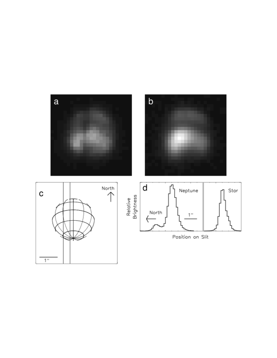
Figure 1: (a) SCAM image of Neptune with spectrometer slit overlying Neptune. This image was taken in the NIRSPEC-6 filter (1.558-2.31 $\mu$m) at 14:06 UT during the first Neptune spectral exposure. (b) SCAM image of Neptune unobstructed by slit. This image was taken in the NIRSPEC-7 filter (1.839-2.630 $\mu$m) at 13:45 UT. No unobstructed images of Neptune were taken in the NIRSPEC-6 filter. (c) Schematic showing the scale and orientation of Neptune in (a) and (b). North is up and Neptune appears as it would look on the sky. The scale of the schematic is shown at lower-left and is the same as in (a) and (b). The vertical lines show the approximate location of the slit in (a). (d) Brightness of Neptune along the slit, averaged over all the wavelengths shown in the spectral image in Fig. 2b. For comparison to atmospheric seeing, the profile of the star HD201941, averaged over the same wavelength range, is also shown. The profile of HD201941 gives a seeing FWHM of $\sim 0\farcs 5-0\farcs 6$. The FWHM of the unidentified star in the the scam images taken simultaneously with the Neptune spectra was 0$\farcs$4. The narrowness of the FWHM compared to the separation of Neptune’s northern and southern features, along with the clear local minimum between the features, leads us to conclude that we have separated the light from these two features relatively well.

The spectra presented here come from two 60-second exposures taken with a 42$\farcs$ $\times$ 0$\farcs$380 slit starting at 14:06 (UT) on 1999 June 2. The slit was aligned parallel with Neptune’s north-south axis and centered on the bright feature in the southern hemisphere. This feature was by far the brightest that we observed on Neptune on 1999 June 2 (UT). The slit also captured light from a dimmer feature in Neptune’s northern hemisphere. Between the two exposures the pointing of the telescope was moved $\sim$10” along the direction of the slit, so that Neptune fit easily on the slit for both exposures. In order to correct for Earth’s atmospheric absorption, we observed an A2 spectral type star (HD201941) in two 10 second exposures, with an offset of the telescope pointing between exposures in order to move the star along the slit.

The reduction sequence consisted simply of subtraction of one star spectral frame from the other for bias and background subtraction. In these images the spatial and spectral coordinates are distorted with respect to the rows and columns of the detector array. The OH sky emission lines in unsubtracted frames trace out lines of constant wavelength and are well fit by straight lines

$$Y(x)=A_{0}(\lambda)+A_{1}(\lambda)x,$$ (1)

where A₀ and A₁ are functions of wavelength. Meanwhile, the arc of a stellar spectrum traces out a line of constant position along the slit and is well fit by the function

$$X(y)=B_{0}(s)+B_{1}(s)y+B_{2}(s)y^{2},$$ (2)

where B₀, B₁, and B₂ are all functions of slit position (s). The (x,y) position on the array for a given slit-position and wavelength (s,$\lambda$) can then be found by: interpolating A₀ and A₁ for $\lambda$ from the numerous OH lines that we fit, interpolating B₀, B₁, and B₂ from the several stellar spectra fit, and finally finding the (x,y) intersection of Eqns. 1 and 2. By doing this for a grid of wavelengths and positions along the slit the data in a spectral image is interpolated from (x,y) to (s,$\lambda$). The final step in this rectification process is to apply a Jacobian correction for the geometric distortion. We extracted the stellar spectrum from the rectified spectral image using an optimal weighted extraction technique that includes a median filter rejection algorithm to remove the effects of bad pixels and cosmic ray hits. Finally, we divided the extracted stellar spectrum by that of Vega (spectral type A0V) (Colina, Bohlin, $\&$ Castelli, 1996b) to produce an estimate of the combined atmospheric and instrumental transfer function, shown in Fig. 2a.

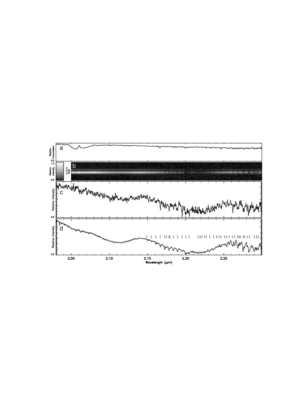
Figure 2: (a) Observed spectrum of A2 star HD201941 divided by the reference spectrum of A0V star Vega, providing an estimate of the atmospheric and instrumental transmission functions. (b) Rectified spectral image of Neptune. The spectral region of 2.03 to 2.05 $\mu$m is omitted in order to show an intensity-bar and the spatial size of Neptune’s diameter along the slit. (c) Extracted spectrum of the dimmer northern feature. d) Extracted spectrum of the brighter southern feature. Note the short vertical tick marks that show methane absorption lines identified from the laboratory spectrum of McKellar (1989). The vertical scale in (c) is exaggerated by a factor of 11 with respect to the vertical scale in (d).

We processed the spectrum of Neptune in a manner similar to that applied to the calibration star; however, after rectification, but before extraction, we inserted the additional step of dividing by the transfer function determined from the star. The final rectified spectral image of Neptune is shown in Fig. 2b. We extracted the spectra of the cloud features in a similar manner as for the stellar spectrum, except that we limited the extractions to 0$\farcs$6 along the slit centered on each feature. The spectrum of the dimmer northern cloud feature is shown in Fig. 2c, and the spectrum of the brighter southern feature is shown in Fig. 2d. Shown in Fig. 2c and 2d are averages from the two separate exposures. Having two separate exposures provides a check on our precision. The two spectra of the northern feature extracted from the two exposures appeared identical except for random noise. Similarly, the two southern feature spectra were also very nearly identical.

Navigation on the images of Neptune is difficult because light from the cloud so dominates over all other features, however the presence of Triton in the slit-viewing camera images makes this problem significantly easier. By centroiding a gaussian on Triton and using the offset from Triton to Neptune’s center given by JPL’s Horizons ephemeris, we find the center of Neptune. Combining this with centroiding a Gaussian on the cloud feature we estimate the cloud to be located 0$\farcs$65$\pm$0$\farcs$25 from the center of Neptune’s disk at a Neptune latitude of -48$\fdg\pm$6$\fdg$. Thus, the cloud lay at a viewing angle $\Theta$ of 34$\fdg\pm$17$\fdg$, where $\Theta$ is the angle between the normal on Neptune’s ‘surface’ and our line of sight. By a similar procedure we estimate the observed northern feature to be at a latitude of 30$\fdg\pm$13$\fdg$ and a viewing angle of 55$\fdg^{+9\fdg}_{-4\fdg}$.

3 Atmospheric Model

Our aim in the work presented here is to measure the altitude or pressure level at the top of an infrared-bright cloud on Neptune. Towards this end we have taken spectra, presented in the previous section, over a wavelength range where the opacity in Neptune’s atmosphere varies significantly as a function of wavelength due to H₂ collision induced absorption (H₂-CIA) and methane absorption. In our model we calculate the predicted spectrum as a function of the altitude of the top of the cloud and several other parameters described below. We judge the goodness-of-fit for each model spectrum using the metric $\sum(I_{obs}(\lambda)-A\cdot I_{model}(\lambda))^{2}$, where $A$ is chosen in each case to minimize the overall sum. The introduction of the factor $A$ is necessary due to the lack of an absolute flux calibration for the observed spectrum, I${}_{obs}(\lambda)$.

Our model atmosphere consists of 120 layers evenly spaced in Log₁₀(P_bar) from 5.0 to $10^{-4}$ bar. We interpolate the temperature and pressure for each layer from Lindal (1992). The free parameters in our model are: the mole fraction of helium, F_He; the mole fraction of methane in the stratosphere, F${}_{CH_{4},s}$; the mole fraction of methane in the troposphere, F${}_{CH_{4},t}$; the fraction of H₂ in ortho/para thermodynamic equilibrium, F_eq; the viewing angle, $\Theta$; and the pressure altitude of the top of the cloud in bar, P_bar. Around the tropopause the fractional methane abundance follows the saturation vapor curve, so that the methane abundance is never super-saturated. Wavelengths of 2.03-2.30 $\mu$m do not probe significantly into the troposphere, and therefore our model fit is insensitive to changes in F${}_{CH_{4},t}$. In each layer a fraction of the H₂, F_eq, is distributed between ortho and para states according to thermodynamic equilibrium, with the remaining H₂ distributed according to an ortho:para ratio of 3:1. We calculated the model predicted spectrum for each point on a grid of these free parameters. The grid points for each parameter are listed in Table 1.

Table 1: Model parameter grid points.

Parameter	Values used in model
FHe a	0.08, 0.10, 0.12, 0.14, 0.16, 0.18, 0.20, 0.22
F${}_{CH_{4},s}$ b	$2.\times 10^{-5},8.\times 10^{-5},1.8\times 10^{-4},3.5\times 10^{-4},7.0\times 10^{-4},1.05\times 10^{-3},1.7\times 10^{-3}$
F${}_{CH_{4},t}$ c	0.022
Feq d	0.0, 0.5, 0.6, 0.7, 0.8, 0.9, 1.0
$\Theta$	17$\fdg$, 34$\fdg$, 51$\fdg$
Pbar	120 layers evenly spaced in $Log_{10}(P)$ from 5.0 to 10-4 bar

.

To model collision-induced absorption by hydrogen (H₂-CIA) for H${}_{2}-$H₂ and H${}_{2}-$He collisions we use the FORTRAN routines of A. Borysow (Borysow, 1991, 1993; Zheng $\&$ Borysow, 1995; Borysow et al., 1989a, b). Although both 0-1 and 0-2 transitions are included in our model, for wavelengths of 2.1–2.3 $\mu$m only the 0-1 transition is relevant.

Accurate modeling of methane absorption across the near-infrared spectrum is extremely difficult due to the enormous number of individual lines and huge variation in line strength. We apply the correlated k distribution method as described in Lacis $\&$ Oinas (1991) and on p. 230 of Goody $\&$ Yung (1989). We use the H₂-broadened methane k-coefficients of Irwin et al. (1996) since Neptune’s atmosphere is primarily H₂. These coefficients are for 5 cm^-1 wide bins and this places a limit on the spectral resolution of the model.

We ignore all scattering processes, except reflection from the top of the cloud. Although significant at shorter wavelengths, Rayleigh scattering is negligible at wavelengths of 2.0 to 2.3 $\mu$m. Light reflected from the top of the cloud dominates all other sources which might contribute to our cloud spectrum, such as scattered light from stratospheric hydrocarbon hazes. Therefore, the only scattering process that we include is reflection from the top of the cloud, which we model as a flat reflecting layer. The reflectivity of the top of the cloud, or alternatively, the combined optical depth, scattering phase function, and single scattering albedo, are irrelevant given that we fit the shape of the spectrum, not the absolute flux level. Further, we assume that the optical depth, scattering phase function, and single scattering albedo do not vary significantly over the wavelength range of our spectrum (2.03 to 2.3 $\mu$m). Using the solar spectrum of Colina, Bohlin, $\&$ Castelli (1996a), the model produces the estimated spectrum of the cloud as a function of the pressure level of the top of the cloud.

4 Results of Model Fit

The spectral resolution of the model described in the previous section is limited by the k-coefficients of Irwin et al. (1996) and is coarser than the spectral resolution of our observed spectra. Therefore, we bin the observed spectra in wavelength to achieve a resolution as nearly identical as possible to the model spectra. We restrict the model fitting to the wavelength range 2.08-2.25 $\mu$m in order to avoid a large telluric CO₂ band at $<2.08\mu$m and a series of sharp methane features at $>2.25\mu$m that are poorly represented by the methane coefficients in the model.

For the bright southern feature at a viewing angle of $\Theta=34\fdg$, we obtain our best-fit for a cloud top at 0.14 bar, F${}_{CH_{4},s}=0.0017$, F${}_{He}=0.22$, and F${}_{eq}=1.0$. For the dimmer northern feature at a viewing angle of $\Theta=55\fdg$, the best fit is for a cloud-top pressure of 0.084 bar, F${}_{CH_{4},s}=0.0017$, F${}_{He}=0.22$, and F${}_{eq}=1.0$. These best-fit model spectra are superposed on the observed spectra in spectrum (1) of Fig. 3a and spectrum (1) of Fig. 3b. The two parameters that we can best constrain are P_bar at the top of cloud and the fractional equilibrium of H₂ in ortho/para equilibrium, F_eq. The model spectra do not fit the observations for cloud-top pressures outside the range of 0.11-0.19 bar for the bright southern feature (see spectra (2) and (3) of Fig. 3a), nor outside the range of 0.058-0.110 bar for the dimmer northern feature (see spectra (2) and (3) of Fig. 3b). As shown in Fig. 4, reasonable model fits to both the northern and southern spectra require F${}_{eq}>\sim$0.8. We find that our data do not constrain significantly F_He and F${}_{CH_{4},s}$.

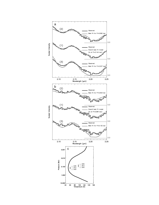
Figure 3: Constraint on the cloud top pressure. (a) In each case the solid dark line is the binned observed spectrum of the bright southern feature. The overplotted grey lines are the model spectra: (1) The overall best fit model is for P_bar=0.144 bar, F${}_{CH_{4},s}=1.7\times 10^{-3}$, F_He=0.22, F_eq=1.0, and $\Theta=34\fdg$. (2) When the cloud top is raised to 0.092 bar, the best fit is poor and requires F${}_{CH_{4},s}=1.7\times 10^{-3}$, F${}_{He}=0.08$, F${}_{eq}=1.0$, and $\Theta=34\fdg$. (3) Similarly, when the cloud top is lowered to 0.227 bar, the best fit is poor. In this case F${}_{CH_{4},s}=2.\times 10^{-5}$, F${}_{He}=0.22$, F${}_{eq}=1.0$, and $\Theta=34\fdg$. (b)In each case the solid dark line is the binned observed spectrum of the dimmer northern feature. The overplotted grey lines are the model spectra: (1) The overall best fit model is for P_bar=0.084 bar, F${}_{CH_{4},s}=1.7\times 10^{-3}$, F_He=0.22, F_eq=1.0, and $\Theta=55\fdg$. (2) When the cloud top is raised to 0.053 bar, the best fit is poor and requires F${}_{CH_{4},s}=1.7\times 10^{-3}$, F${}_{He}=0.08$, F${}_{eq}=1.0$, and $\Theta=55\fdg$. (3) Similarly, when the cloud top is lowered to 0.132 bar, the best fit is poor. In this case F${}_{CH_{4},s}=1.05\times 10^{-3}$, F${}_{He}=0.22$, F${}_{eq}=0.9$, and $\Theta=55\fdg$. (c) The temperature-pressure profile of Lindal (1992). Also plotted are the cloud top pressures of the model spectra in Fig. 3a. The short vertical line on the far left shows the narrow range of pressures to which our observations restrict the top of the cloud.

Due to the low spatial resolution of our data there is significant uncertainty in the viewing angle for both features, $\Theta=34\fdg\pm 17\fdg$ for the bright southern feature and $\Theta=55\fdg^{+9\fdg}_{-4\fdg}$ for the dimmer northern feature. Decreasing $\Theta$ to $17\fdg$ for the bright southern feature pushes the best-fit cloud-top pressure to 0.16 bar, while increasing $\Theta$ to 51$\fdg$ changes the best-fit cloud-top pressure to 0.12 bar. Similarly for the northern feature, decreasing $\Theta$ to 51$\fdg$ moves the best-fit cloud-top pressure to 0.092 bar, while increasing $\Theta$ to 64$\fdg$ shifts the best-fit cloud-top pressure to 0.076 bar. In all these cases the best-fit parameters include F${}_{eq}=1.0$ and F${}_{CH_{4},s}=0.0017$.

5 Errors and Uncertainties

At this point it is worthwhile to make a brief discussion of how the errors and uncertainties in our observations and model fitting could affect our results with respect to cloud-top pressure and F_eq.

On the observing side, we are much more concerned with systematic errors, for instance artificial slopes across the entire spectrum, than with random errors in the spectra of HD201941 and Neptune. Since we are fitting the model to 73 wavelength bins, random errors from bin to bin will tend to cancel out and not bias the model fit. There are several possible sources of systematic errors on the observing side; the three of greatest concern relate to alignment on the slit and the method of atmospheric correction. Misalignment of the slit on the star would redden the spectrum and possibly introduce a bias in the final model fitting. This is less of an issue on an extended source such as the clouds on Neptune. By looking at multiple stellar spectra we estimate that this source of error introduces at most a one to two percent slope from 2.08 to 2.25 $\mu$m.

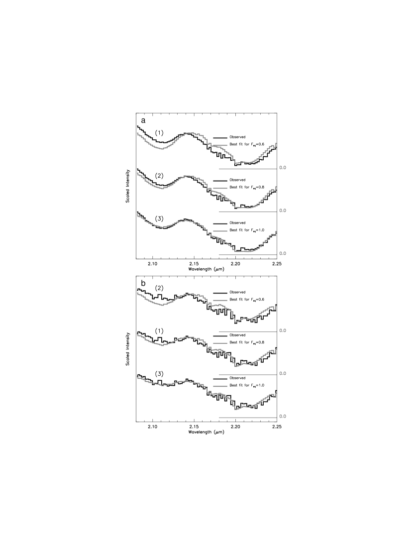
Figure 4: Constraint on the fraction of H₂ in ortho/para equilibrium (F_eq). (a) In each case the solid dark line is the binned observed spectrum of the bright southern feature. Holding F_eq fixed at 0.6, 0.8, 1.0, the best fits of model to data are shown. In all three cases the best fit included P_bar=0.144 bar and F${}_{CH_{4},s}1.7\times 10^{-3}$. In cases (1) and (3) F_He=0.22, while in case (2) F_He=0.20, which is not a significant difference. (b) In each case the solid dark line is the binned observed spectrum of the dimmer northern feature. Holding F_eq fixed at 0.6, 0.8, 1.0, the best fits of model to data are shown. In all three cases the best fit was P_bar=0.144 bar, F${}_{CH_{4},s}1.7\times 10^{-3}$, and F_He=0.22.

In applying the atmospheric and instrumental transmission correction with HD201941 there are two more potential sources of systematic error. The first is that to find the atmospheric transmission function we divided HD201941 by a spectrum of Vega, and the second is that HD201941 was not observed at exactly the same airmass and time as Neptune. While Vega is an A0V star, HD201941 is listed as an A2 star in the SIMBAD database. In order to estimate the maximum slope bias that this stellar mis-match could introduce, we compared blackbody curves. Drilling $\&$ Landolt (2000) give the T_eff for an A0V star as 9790 K and for an A2V star as 9000 K. This difference suggests a slope error of 0.29 percent from 2.08 to 2.25 $\mu$m. The spectra of HD201941 were taken at an airmass 1.05, while the Neptune spectra were taken at airmass 1.28. In order to minimize the influence of this on the model fitting we excluded wavelengths shortward of 2.08 $\mu$m to avoid a large CO band. To investigate what biases and slopes this mismatch in airmass could introduce we used the ATRAN (Lord, 1992) model atmospheric transparency spectra available on the Gemini Observatory website. While we did not examine transparency spectra for our exact airmasses, the slope difference introduced by observing at airmass 1.0 versus 1.5 across our spectral range of interest would be 1.6 percent.

Each of these possible slope errors discussed above is less than 2 percent. To show that even a fortuitous addition of all these slope errors in one direction would not change our primary results we artificially introduced slope errors of $\pm$10 percent to our final observed spectra and refit the model. This had no effect on results concerning F_eq and at most shifted the best-fit pressure level of the cloud top by one level in our model, to 0.12 bar in the $-10\%$ case for the bright southern feature and to 0.09 bar in the $+10\%$ case for the dimmer northern feature.

While there are numerous small ways in which the model may be inaccurate, for instance if the temperature-pressure curve is not exactly correct for the location of the cloud features, the two major sources of uncertainty in the model are the methane k-coefficients of Irwin et al. (1996) and the assumption of a flat reflecting cloud layer. For Neptune’s atmosphere we are forced to extrapolate the methane k-coefficients to much colder temperatures than the temperatures of the laboratory measurements on which they are based. While the accuracy or inaccuracy of this extrapolation is difficult to judge, the independence of best-fit cloud-top pressure and F_eq from methane concentration F${}_{CH_{4},s}$ gives us confidence in our results.

For ease we assume in our model that the cloud top is a flat reflecting layer, however due to particle scattering properties the reflectivity of the cloud may vary with wavelength and the ‘top’ of the cloud is almost certainly somewhat extended. Our best-fit model for the bright southern feature (see spectrum 1 of Fig. 3a) is systematically slightly off from the observed spectrum. This is most easily seen at wavelengths shortward of $\sim$2.16 $\mu$m where H₂ absorption dominates. This is suggestive that while a flat reflecting layer at 0.144 bar does not fit perfectly, a combination of reflectance from pressures slightly higher to slightly lower than 0.144 bar might result in a better fit, which is exactly what one would expect if the cloud-top were somewhat extended. In fact, a more detailed method of modeling would be to view the computed model spectra for all the pressure levels in the model as a basis set and to construct the best-fit model spectrum from a linear combination of all the spectra from different levels. However, one shortfall to that approach is that it implicitly assumes single scattering, ignoring multiple scattering between layers. A more complete modeling approach must include the multiple scattering between layers as well, which is beyond the scope of the current paper. Variation in reflectivity as a function of wavelength may also play a role in these slight discrepancies between model and data.

6 Conclusions

By comparing a near-infrared spectrum with the predictions of a simple transmission model we determined the pressure level at the top of an infrared-bright tropospheric cloud on Neptune. We find a best-fit of model to data for a cloud-top pressure level of 0.14 bar within a maximum allowed range of 0.11 to 0.19 bar for the bright southern feature that we observed. We found the dimmer northern feature to sit slightly higher in the atmosphere at 0.084 bar within a maximum allowed range of 0.058 to 0.11 bar. Our work places no limit on the pressure at the bottom of the cloud. Our results further restrict the fraction of H₂ in ortho/para equilibrium to greater than 0.8, and our best-fits consistently put this fraction at 1.0. This is in agreement with the work of Baines $\&$ Smith (1990) who found the same results, but from a different technique, measuring the equivalent widths of the 4-0 S(0) and S(1) transitions between 0.6 and 0.7 $\mu$m. Our results do not constrain the fractional abundance of methane in the stratosphere, nor the fractional abundance of helium.

Our primary result is the tight constraint we place on the pressure at the top of the cloud. By constraining the cloud-top to pressures around the tropopause, we show that the cloud, possibly a storm or upwelling, does not extend significantly into the stratosphere. If the cloud is made up of condensed methane particles brought up from below, then the mechanism by which this cloud was formed appears to be efficient at bringing methane to near the top of the troposphere, but, at least at the time we observed, the mechanism was not acting as an efficient method of transporting methane to the upper stratospheric levels where ultraviolet photolysis occurs (P$>10^{-2}-10^{-3}$ bar).

In the current paper we present a measurement of the altitude of two cloud features at a single time. We expect longer-term observations of multiple infrared-bright features will find that most reach only to approximately the tropopause, as in the case presented here, but occasional features may reach far into the stratosphere (P$>0.01$ bar) and thus would provide an extremely efficient method of transporting methane to the upper stratosphere for photolysis. We are currently undertaking such a program of observations using NIRSPEC coupled to the Keck Adaptive Optics system (Wizinowich et al., 2000) to achieve simultaneous high-spatial and high-spectral resolution.

References

- Baines Smith (1990) Baines, K. H., Smith, Wm. H. 1991, Icarus, 85, 65
- Baines Hammel (1994) Baines, K. H., Hammel, H. B. 1994, Icarus, 109, 20
- Baines et al. (1995a) Baines, K.H., Mickelson, M. E., Larson, L. E., Ferguson, D. W. 1995a, Icarus, 114, 328
- Baines et al. (1995b) Baines, K.H., Hammel, H. B., Rages, K. A., Romani, P. N., Samuelson, R. E. 1995b, in Neptune and Triton, ed. D.P. Cruikshank (Univ. of Arizona Press, Tucson), 489
- Borysow (1991) Borysow, A. 1991, Icarus, 92, 273
- Borysow (1993) Borysow, A. 1993, Icarus, 106, 614
- Borysow et al. (1989a) Borysow, A., Frommhold, L., Moraldi, M. 1989, ApJ, 336, 495
- Borysow et al. (1989b) Borysow, A., Frommhold, L. 1989, ApJ, 341, 549
- Colina, Bohlin, Castelli (1996a) Colina, L., Bohlin R.C., Castelli, F. 1996a, AJ, 112, 307
- Colina, Bohlin, Castelli (1996b) Colina, L., Bohlin R.C., Castelli, F. 1996b, Instrument Science Report OSG-CAL-96-01, STSCI
- Conrath et al. (1993) Conrath, B. J., Gautier, D., Owen, T.C., Samuelson, R. E. 1993, Icarus, 101, 168
- Drilling Landolt (2000) Drilling, J. D., Landolt, A. U. 2000, in Astrophysical Quantities, ed. A. N. Cox, (New York: Springer-Verlag), 381
- Gibbard et al. (2000) Gibbard, S. G., de Pater, I., Roe, H., Macintosh, B., Gavel, D., Max, C. E., Baines, K. H., Ghez, A. 2000, Icarus, submitted
- Goody Yung (1989) Goody, R. M., Yung, Y. L. 1989, Atmospheric Radiation, (Oxford University Press)
- Hammel Buie (1987) Hammel, H. B., Buie, M. W. 1987, Icarus, 72, 62
- Hammel (1989) Hammel, H. B. 1987, Icarus, 80, 14
- Hammel et al. (1989) Hammel, H. B., Baines, K. H., Bergstralh, J. T. 1989, Icarus, 80, 416
- Hammel (1990) Hammel, H. B. 1987, Advances in Space Research, 10, 99
- Hammel Lockwood (1997) Hammel, H. B., Lockwood, G. W. 1997, Icarus, 129, 466
- Hammel et al. (1995) Hammel, H. B., Lockwood, G. W., Mills, J. R., Barnet, C. D. 1995, Science, 268, 1740
- Irwin et al. (1996) Irwin, P. G. J., Calcutt, S. B., Taylor, F. W., Weir, A. L. 1996, J. Geophys. Res., 101, 26137
- Joyce et al. (1977) Joyce, R. R., Pilcher, C. B., Cruikshank, D. P., Morrison, D. 1977, ApJ, 214, 657
- Lacis Oinas (1991) Lacis, A.A., Oinas, V. 1991, J. Geophys. Res., 96, 9027
- Lindal (1992) Lindal, G.F. 1992, AJ, 103, 967
- Lord (1992) Lord, S. D. 1992, NASA Tech Memorandum 103957
- Max (2000) Max, C. E. et al. 2000, in Proc. SPIE 4007, Adaptive Optical Systems Technology, ed. P. L. Wizinowich (Bellingham, WA: SPIE), 803
- McKellar (1989) McKellar, A.R.W. 1989, Can. J. Phys. 67, 1027
- McLean et al. (1998) Mclean, I. S., et al. 1998, Proc. SPIE, 3354, 566
- Moses et al. (1995) Moses, J.I., Rages, K., Pollack, J.B. Icarus, 113, 232
- Pilcher (1977) Pilcher, C. B. 1977, ApJ, 214, 663
- Roddier et al. (1997) Roddier, F., Roddier, C., Brahic, A., Dumas, C., Graves, J. E., Northcott, M. J., Owen, T. 1997, Planet. Space Sci., 45, 1031
- Roddier et al. (1998) Roddier, F., Roddier, C., Graves, J. E., Northcott, M. J., Owen, T. 1998, Icarus, 136, 168
- Roe et al. (2000) Roe, H.G., Gavel, D., Max, C., de Pater, I., Gibbard, S., Macintosh, B., Baines, K. 2000, AJ, submitted
- Romani et al. (1993) Romani, P.N., Bishop, J., Bezard, B., Atreya, S. 1993, Icarus, 106, 442
- Smith (1984) Smith, B.A. 1984, in Uranus and Neptune, NASA, 213
- Smith (1985) Smith, B.A. 1985, Astronomicheskii Vestnik, 19, 42
- Smith et al. (1989) Smith, B., et al. 1989, Science, 246, 1422
- Sromovsky et al. (1995) Sromovsky, L. A., Limaye, S. S., Fry, P. M. 1995, Icarus, 118, 25
- Sromovsky et al. (2001a) Sromovsky, L. A., Fry, P. M., Baines, K. H., Limaye, S. S., Orton, G. S., Dowling, T. E. 2001, Icarus, 149, 416
- Sromovsky et al. (2001b) Sromovsky, L. A., Fry, P. M., Baines, K. H., Dowling, T. E. 2001, Icarus, 149, 435
- Sromovsky et al. (2001c) Sromovsky, L. A., Fry, P. M., Dowling, T. E., Baines, K. H., Limaye, S. S. 2001, Icarus, 149, 459
- Wizinowich et al. (2000) Wizinowich, P., et al. 2000, in Proc. SPIE 4007, Adaptive Optical Systems Technology, ed. P. L. Wizinowich (Bellingham, WA: SPIE), 2
- Zheng Borysow (1995) Zheng, C., Borysow, A. 1995, Icarus, 113, 84