The Kinematics of High Proper Motion Halo White Dwarfs

Abstract

We analyse the kinematics of the entire spectroscopic sample of 99 recently discovered high proper-motion white dwarfs by Oppenheimer et al. using a maximum-likelihood analysis, and discuss the claim that the high-velocity white dwarfs are members of a halo population with a local density at least ten times greater than traditionally assumed. We argue that the observations, as reported, are consistent with the presence of an almost undetected thin disc plus a thick disc, with densities as conventionally assumed. In addition, there is a kinematically distinct, flattened, halo population at the more than 99% confidence level. Surprisingly, the thick disc and halo populations are indistinguishable in terms of luminosity, color and apparent age (1–10 Gyr). Adopting a bimodal, Schwarzschild model for the local velocity ellipsoid, with the ratios $\sigma_{\rm U}$:$\sigma_{\rm V}$:$\sigma_{\rm W}$=1:2/3:1/2, we infer radial velocity dispersions of $\sigma_{\rm U}$=62${}^{+8}_{-10}$ km s^-1 and 150${}^{+80}_{-40}$ km s^-1 (90% C.L.) for the local thick disc and halo populations, respectively. The thick disc result agrees with the empirical relation between asymmetric drift and radial velocity dispersion, inferred from local stellar populations. The local thick-disc plus halo density of white dwarfs is $n^{\rm td+h}_{\rm 0,WD}$=$(1.9\pm 0.5)\times$$10^{-3}$ pc^-3 (90% C.L.), of which $n^{\rm h}_{\rm 0,WD}$=1.1${}^{+2.1}_{-0.7}$$\times$$10^{-4}$ pc^-3 (90% C.L.) belongs to the halo, a density about five times higher than previously thought. Adopting a mean white-dwarf mass of 0.6 M_⊙, the latter amounts to 0.8${}^{+1.6}_{-0.5}$$\times$10^-2 (90% C.L.) of the nominal local halo density. Assuming a simple spherical logarithmic potential for the Galaxy, we infer from our most-likely model an oblate halo white-dwarf density profile with $n(r)\propto r^{-\alpha}$ and $\alpha\approx 3.0$. The halo white dwarfs contributes $\sim 2.6\times 10^{9}$ M_⊙, i.e. a mass fraction of $\sim$0.004, to the total mass inside 50 kpc ($\Omega_{\rm WD}\sim 10^{-4}$). The halo white dwarf population has a microlensing optical depth towards the LMC of $\tau^{\rm h}_{\rm WD}\approx 1.3\times 10^{-9}$. The thick-disc white dwarf population gives $\tau^{\rm td}_{\rm WD}\approx 4\times 10^{-9}$. The integrated Galactic optical depth from both populations is 1–2 orders of magnitude below the inferred microlensing optical depth toward the LMC. If a similar white-dwarf population is present around the LMC, then self-lensing can not be excluced as explanation of the MACHO observations. We propose a mechanism that could preferentially eject disc white dwarfs into the halo with the required speeds of $\sim$200 km s^-1, through the orbital instability of evolving triple star systems. Prospects for measuring the density and velocity distribution of the halo population more accurately using the Hubble Space Telescope Advanced Camera for Surveys (ACS) appear to be good.

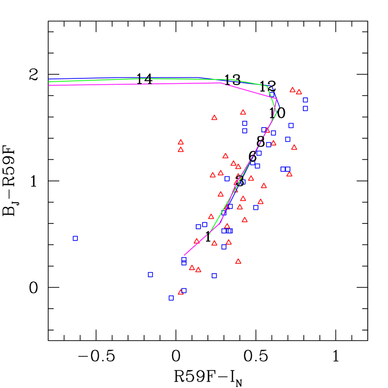
Figure 1: Color-color diagram of the sample of WDs. Shown are the high-velocity ($>$94 km s^-1; squares) and low-velocity WDs ($<$94 km s^-1; triangles). The velocity cuts in $U$ and $V$ (see Sect.2) are taken as in Oppenheimer et al. (2001), for reasons of consistency, but assume $v_{r}=0$ km s^-1. The cooling curves are those from Chabrier et al. (2000). The upper to lower curves represent 0.5, 0.6 and 0.8–M_⊙ WDs with pure hydrogen atmospheres. Ages in Gyr are indicated along the 0.5-M_⊙ curve.

1 Introduction

As the most common stellar remnants, white dwarfs (WD) provide an invaluable tracer of the early evolution of the Galaxy. Their current density and distribution reflects the disposition of their progenitor main sequence stars and their colors indicate their ages, which are consistent with many of them having been formed when the Galaxy was quite young (e.g. Wood 1992).

Until recently, it has been assumed that halo WDs contribute a negligible fraction of the total mass of the Galaxy (e.g. Gould, Flynn & Bahcall 1998). This view is supported by the constraint that the formation of $\sim$0.6–M_⊙ WDs is accompanied by the release of several solar masses of gas, heavily enriched in CNO elements (e.g. Charlot & Silk 1995; Gibson & Mould 1997; Canal, Isern & Ruiz-Lapuente 1997). Yet local stars and interstellar gas, which only comprise $\sim 10$% of the total Galaxy mass, contain only 2–3 percent of these elements by mass. Based on these metalicity arguments, most recently Fields, Freese & Graff (2000) have argued that $\Omega_{\rm WD}$$<$$3\times 10^{-4}$ from C and N element abundances, adopting H₀=70 km s^-1 Mpc^-1. WDs can therefore not comprise more than 1–10% percent of the dark matter in the Galactic halo within 50 kpc, if $\Omega_{\rm halo}(<50{\rm~{}kpc})\sim 0.03$ (e.g. Bahcall et al. 2000). However, this argument can be circumvented if significant metal outflow from the Galaxy, due to supernovae, accompanies the formation of these WDs, thereby removing most of the produced metals from the Galaxy (e.g. Fields, Mathews & Schramm 1997).

These considerations are important because the MACHO collaboration (e.g. Alcock et al. 2000) report a frequency of Large Magellanic Cloud (LMC) microlensing events that is suggestive of 8–50% (95% C.L) of the halo mass in $\sim 0.5$–M_⊙ compact objects inside a 50 kpc Galacto-centric radius. Faint stars and brown dwarfs seem to comprise only a few percent of the Galaxy mass (e.g. Bahcall et al. 1994; Graff & Freese 1996a, 1996b; Mera, Chabrier & Schaeffer 1996; Flynn, Gould & Bahcall 1996; Freese, Fields & Graff 1998) and are therefore unlikely to be responsible for these microlensing events. The only remaining candidates with similar masses, known to us, are WDs.

Alternative explanations for these microlensing events, based on stellar self-lensing in the LMC have been put forward (Wu 1994; Sahu 1994; Salati et al. 1999; Aubourg et al. 1999; Evans & Kerins 2000). A comparable microlensing survey done by the EROS collaboration only claims an upper limit of 40% (95% C.L.) of the halo mass in compact objects with mass less than 1 M_⊙ (Lasserre et al. 2000; see Afonso et al. 1999 for SMC results). Because the EROS survey targets the outer regions of the LMC, in contrast to the MACHO survey, this could indeed suggest some self-lensing contribution.

There have also been claims of a number of high proper-motion objects in the HDF, which were suggested to be old WDs in the Galactic halo at a distance of $\sim$2 kpc (Ibata et al. 1999), with blue colors that were consistent with revised white-dwarf atmosphere models (Hansen 1999). More locally, Ibata et al. (2000) found two high proper-motion WDs. If the HDF results had been confirmed, they alone would have been sufficient to explain the observed microlensing optical depth towards the LMC. However, recent third-epoch observations have shown that these “objects” were misidentifications and not moving objects (Richer 2001).

The topic has become interesting again, though, with the recent discovery by Oppenheimer et al (2001) of 38 nearby, old WDs, with de-projected horizontal velocities in excess of 94 km s^-1 (see Sect.2). They concluded that at least two percent of the halo is composed of these cool WDs. This conclusion has been challenged, however, by Reid, Sahu & Hawley (2001), who claim that these WDs could be the high-velocity tail of the thick disk. In addition, Hansen (2001) has argued that these WDs follow the same color-magnitude relation as those of the disc, which might be unexpected if they are a halo population.

In this paper, we take the observations of Oppenheimer et al. (2001) at face value and examine their conclusions in more detail. We assume that the high proper motion objects have correctly been identified as WDs and that their inferred distances are statistically unbiased. However, it is important that additional observations be performed to validate this. We also discuss how to set more precise bounds on the halo WD density.

2 The White–Dwarf Sample

The high proper motion WDs were selected from digitized photographic plates from the SuperCOSMOS Sky Survey (Hambly et al. 2001), covering an effectively searched area of 4165 square degree around the South Galactic Pole (SGP), upto $b$ $\approx$$-$45^∘. Objects with proper motions between $\mu$=0.33 and 10.0  arcsec yr^-1 were selected, that were brighter than $R59F$=19.8 mag and seen at three epochs in each field. From these objects a sample of 126 potential halo WDs was drawn based on their reduced proper motion ($H_{\rm R}$=$R59F$+5 $\log\mu$+5) and their color $B_{\rm J}-R$. After spectroscopic observations of 69 of the 92 WDs without spectra (34 had published spectra), a sample of 99 WDs remained. For a full discusion of the sample, its selection criteria and completeness, we refer to Oppenheimer et al. (2001).

Distances to each of these WDs were ascribed using the photometric parallax relation derived by Bergeron et al. (1997). This was checked in two cases using measured distances and the relative uncertainty was estimated at 20 percent. Using these distances, Oppenheimer et al. (2001) subsequently performed a velocity selection on the WD sample. The proper motions were converted into a velocity in Galactic coordinates relative to the local standard of rest, (LSR), with $U$ directed towards the Galactic center (GC), $V$ along the direction of the circular velocity and $W$ towards the North Galactic Pole (NGP), see Fig.2. The absence of a measured radial velocity ($v_{r}$) was compensated by assuming that $W$=0 and deprojecting onto the $U-V$ plane. It was then argued that 95 percent of the thick-disc WDs have velocities in the plane within 94 km s^-1 ($\approx 2\sigma_{{\rm td}}$) from the asymmetric drift point $(U,V)$=$(0,-35)\mbox{~{}~{}km s${}^{-1}$}$ and consequently all such WDs were eliminated, leaving a sample of 38 high-velocity WDs of which 26 are new discoveries and 14 exhibit hydrogen lines and are believed to be younger. These WDs have velocities in the Galactic plane that are enclosed within a circle of radius $2\sigma_{{\rm h}}$ centered on $(U,V)=(0,-220)$ km s^-1 corresponding to a non-rotating halo distribution. The density of WDs in the magnitude-limited sample was then estimated to be $\sim 10^{-4}$ M_⊙ pc^-3, roughly ten times the expected density (e.g. Gould, Flynn & Bahcall 1998) and equivalent to 2 percent of the nominal local halo mass density (e.g. Gates, Gyuk & Turner 1995).

This procedure has been criticised by Reid, Sahu & Hawley (2001) who de-project the velocity vector by setting the radial velocity ($v_{r}$) to zero, thereby reducing the number of high velocity WDs. This procedure, however, also places several lower velocity WDs outside the 94 km s^-1 cut. Reid et al. (2001) also note that the high velocity WDs are not concentrated around $(U,V)=(0,-220)$ km s^-1 as might be expected from a halo population and argue that the WDs are mostly associated with the high velocity tail of the thick disc plus a few WDs from the traditional halo stellar population. Essentially the same point has been made by Graff (2001). In addition, Gibson & Flynn (2001) identified a number of errors in the original table of white-dwarf properties and argued that the Oppenheimer et al. (2001) densities are further overestimated by a factor 3–10, bringing them more into line with the results from other surveys.

In this paper, we analyse the full sample of 99 WDs, not only those 38 with the highest space velocities, thereby avoiding potential pitfalls associated with arbitrary cuts in the sample and analysing only subsamples.

Figure 2: The Galactic coordinate system. The $U$, $V$ and $W$ velocity components point toward the Galactic center (GC), in the direction of Galactic rotation (anti-clockwise as seen from the North Galactic Pole, NGP) and out of the Galactic Plane, respectively. The velocity components $v_{\ell}$ and $v_{b}$ are the projected velocity components on the sky, in the Galactic coordinates system $(\ell,b)$, of a WD with space velocity $\vec{v}_{\rm WD}$, and $v_{r}$ is the radial velocity. The vector $\vec{v}_{\odot}$ indicates the Solar motion with respect to the Local Standard of Rest (LSR).

2.1 White-Dwarf Distances and Ages

The photometric parallax method to obtain distances hides a potential problem for the oldest WDs ($\ga$10 Gyr). Although these white dwarfs continue to cool and fade away, their $B_{\rm J}-R59F$ color remains nearly constant at $\approx$1.9 for $M_{B_{\rm J}}$$\ga$18 (Fig.1; e.g. Chabrier et al. 2000). Blindly applying the linear color-magnitude relation given in Oppenheimer et al. (2001) to the oldest WDs would therefore lead to a severe overestimate of their intrinsic luminosity and distance. Even if old WDs are present in the sample, it might not be surprising that they don’t show up in the color-magnitude relation by Hansen (2001). WDs that move onto the horizontal branch of the cooling curve have increasingly overestimated luminositities and consequently move up in the color-magnitude diagram much closer to the sequence of younger ($\la$10 Gyr) WDs. Fortunately, only 5% of the sample of WDs have colors $B_{\rm J}-R59F$$\ga$1.8 (Fig.1) and it should therefore not create a major problem.

However, it is potentially dangerous to create color-magnitude diagrams, using distances that have been derived by forcing the WDs to follow the color-magnitude relation of relatively young WDs, and from those to conclude that the WD are young. This is a circular argument. A better argument is to plot the age sequence on a two-color diagram (Fig.1; see also Oppenheimer et al. 2001). Again, there is no evidence for WDs older than $\sim 10$ Gyr and the high-velocity WDs appear to be drawn from the same population as the low-velocity WDs which are presumably relics of ongoing star formation in the disc. This appears to argue against there being a substantial white-dwarf halo population (e.g. Hansen 2001), although if there exists a mechanism that preferentially gives WDs a high space-velocity during its formation/evolution one might not expect a correlation between age and velocity. The latter would only be expected if velocities increased with time due to slower scattering processes. We return to this in Sect.7.

We should emphasize, however, that the implied ages and distances are only as good as the assumed underlying white-dwarf color-magnitude relation, in this case that from Bergeron et al. (1997), and that independent measurements of their distances are necessary, preferentially through parallax measurements, even though that will be difficult given their large proper motions.

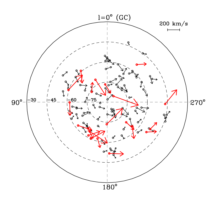
Figure 3: The white-dwarf velocity vectors $(v_{\ell},v_{b})$, with respect to an observer near the Sun, projected on the sky in Galactic coordinates. Galactic latitude increases from $-90^{\circ}$ to $-30^{\circ}$ in steps of $15^{\circ}$ (dashed circles). Galactic longitude increase anti-clockwise with $l=0^{\circ}$ towards to Galactic center (GC). The arrows indicates the velocity and direction of the WDs. The asymmetric drift of the higher velocity WDs ($>$150 km s^-1; thick arrows) is clearly visible, pointing in the direction opposite to Galactic rotation ($\ell=90^{\circ}$).

3 Coordinates and Kinematics

For each WD, we transform its equatorial coordinates ($\alpha$,$\delta$) in to Galactic coordinates ($l$,$b$). Using the distances ascribed by Oppenheimer et al. 2001, we then transform the observed proper motion vector in Galactic coordinates into a vector $(v_{\ell},v_{b})$, where $v_{\ell}$ is velocity component along the $l$-direction and $v_{b}$ is the velocity component along the the $b$-direction (Fig.2). The resulting vector is orthogonal to the line-of-sight, i.e. the direction of the radial velocity ($v_{r}$), which is unknown to us. The transformation from the observed velocities to Galactic velocities ($U$,$V$,$W$) with respect to the Local Standard of Rest (LSR), is

$$U = U_{\odot}+v_{r}\cos b\cos\ell-v_{b}\sin b\cos\ell-v_{\ell}\sin\ell$$

$$V = V_{\odot}+v_{r}\cos b\sin\ell-v_{b}\sin b\sin\ell+v_{\ell}\cos\ell$$

$$W = W_{\odot}+v_{r}\sin b+v_{b}\cos b$$ (1)

where $(U_{\odot},V_{\odot},W_{\odot})=(+10,+5.2,+7.2)$ km s^-1 is the Solar motion with respect to the LSR (Dehen & Binney 1998b). We can use Eq.(3) to transform the velocity distribution function $f(U,V,W)$ (§4.6) in to $f(v_{\ell},v_{b},v_{r})$, or visa versa, at the position of any WD with a measured proper-motion vector and distance.

Fig.3 shows velocity vector ($v_{\ell}$,$v_{b}$) for each WD at its corresponding Galactic coordinates. The velocity vectors point preferentially in the direction opposite to Galactic rotation, which reflects the asymmetric drift (§4.2), whereby a stellar population that is significantly pressure supported, rotates slower than its LSR. If many of the high proper motion objects had been misidentied on the photometric plates, one does not expect a collective movement of these objects in the same direction.

4 A Phase–space Density Model

Before introducing a model for the phase-space density of WDs in the Solar neighborhood in §4.6, we first (i) describe a simple global potential model that we will employ to derive some of the characteristic orbital parameters of the sample of WDs, (ii) reprise epicyclic theory, in order to clarify the discussion and some of the concepts that we will use in this paper, (iii) derive some characteristic quantities of the white-dwarfs data set, (iv) examine the properties of the white-dwarf orbits and (v) discuss some general properties of the Galactic disc components.

4.1 A Toy Model of the Galactic Potential

For definiteness we assume a spherically symmetric potential for the Galaxy

$$\Phi(R,z)=(v_{\rm c}^{2}/2)\cdot\ln(R^{2}+z^{2}),$$ (2)

in cylindrical coordinates, where $R$ is the distance from the rotation axis of the Galaxy and $z$ is the height above the plane. The simplification of spherical symmetry is not inconsistent with observations of the Galaxy and external galaxies, even though a wide range of values for the flattening of the Galactic halo is allowed, often strongly dependent on the method used to derive it (see Olling & Merrifield 2000). This potential, although a clear simplification, it is to first order also consistent with the relatively flat Galactic rotation curve (e.g. Dehnen & Binney 1998a) and allows us to gain insight in the kinematics and properties of the white-dwarf sample. The circular velocity $v_{\rm c}$=$\partial\Phi/\partial\ln R$ in this potential is constant in the plane of the Galaxy ($z$=0).

One can subsequently introduce the effective potential

$$\Phi_{\rm eff}(R,z)=\Phi(R,z)+\frac{L_{\rm z}^{2}}{2R^{2}},$$ (3)

where $L_{\rm z}=R\,v_{\phi}$ is the angular momentum of a WD and $v_{\phi}$ is its tangential velocity in the plane of the Galaxy. If a particle is “at rest” in the minimum of the effective potential, i.e. $\partial\Phi_{\rm eff}/\partial R$=0, one readily finds that $v_{\phi}$=$v_{\rm c}$, hence the WD moves on a circular orbit with a constant velocity $v_{\rm c}$=$\Omega(R)R$, where $\Omega(R)$ is the angular velocity.

4.2 Epicyclic Orbits

Most stars and stellar remnants, however, do not move on perfect circular orbits, but have an additional random velocity and move on orbits around the minimum in their effective potential. If these excursions have relatively small amplitudes, the Taylor expansion of the effective potential around this minimum can be terminated at the second-order derivative and the stars or WDs will exhibit sinusoidal (i.e. epicyclic) motions around the circular orbit. The frequency of these epicyclic motions are $\kappa^{2}=\partial^{2}\Phi_{\rm eff}/\partial R^{2}=(R^{-3}\,{\rm d}(R^{4}\Omega^{2})/{\rm d}R)_{R_{\rm g}}$ in the tangential and radial directions and $\nu^{2}=\partial^{2}\Phi_{\rm eff}/\partial z^{2}$ in the direction out of the plane. The radius of the guiding centre is $R_{\rm g}$ (see §4.2).

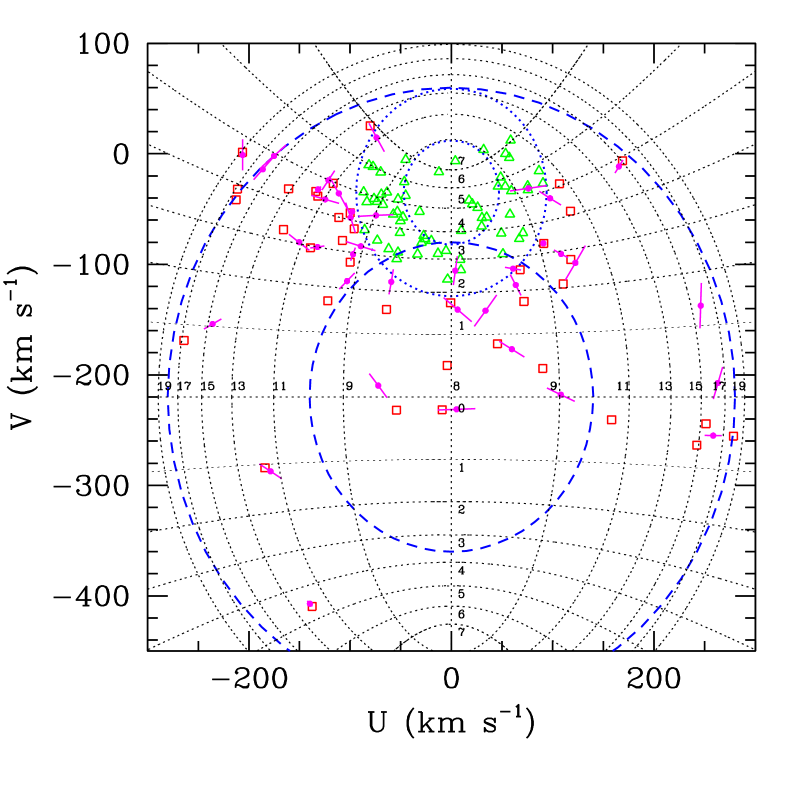
Figure 4: The projection of the 99 white-dwarf velocity vectors on the U–V velocity plane with respect to the LSR (e.g. Oppenheimer et al. 2001; Reid et al. 2001). The squares (triangles) indicates the WDs with velocities in the Galactic plane ($z$=0 and $W$=0) larger (smaller) than 94 km s^-1. The thick dotted and dashed circles correspond to the 1 and 2–$\sigma$ velocity dispersion contours for the disc and halo populations, respectively. The projection assumes that $W$=0. For the population with velocities larger than 94 km s^-1, also the $U$ and $V$ velocities are shown under the assumption that $v_{r}=0\pm 30$ km s^-1(dots with lines). The thin dotted ellipsoidal contours indicate the outermost orbital radii ($R_{\rm max}$, in kpc) of WDs, whereas the paraboloidal contours indicate the innermost orbital radii ($R_{\rm min}$, in kpc). It is assumed that R=8 kpc at the Solar radius and $v_{c}$=220 km s^-1.

Because these frequencies depend on local higher-order derivatives of the potential, we can not use our simple potential model, Eqn.(3), but have to rely on observational constraints (§4.2). One can introduce the Oort’s constants $A$ and $B$, whose values have observationally been determined to be $A$=14.5 km s^-1 kpc^-1 and $B$=$-$12 km s^-1 kpc^-1 in the Solar neighborhood (BT87). From this is follows that $\kappa_{0}^{2}=-4B(A-B)=-4B\Omega_{0}$, i.e. $\kappa_{0}=36$ km s^-1 kpc^-1, and

$${\kappa_{0}\over\Omega_{0}}=2\sqrt{-B\over(A-B)}\approx 1.3.$$ (4)

The frequency of the epicyclic motion is therefore constant at 1.3 times its orbital frequency, irrespective of the amplitude of the orbit around the minimum of its effective potential. In comparison, the potential given by Eq.(2) gives ${\kappa_{0}/\Omega_{0}}=\sqrt{2}\approx 1.4$.

Figure 5: Examples of orbits for two WDs drawn from the sample. (a) High-velocity WD constrained to move in the Galactic plane with $(U,V,W)=(-264,-169,0)$ km s^-1. (b) Slow disk WD dwarf with $(U,V,W)=(49,-21,0)$ km s^-1. (c) The same WD as in (a) except that now we have assigned the velocities on the assumption that the WD is drawn at random from the high-velocity component of the bimodal velocity distribution (§4.5). A projection onto the meridional plane is shown. (d) The same WD as in (b) with velocities drawn from the slow component.

Under the epicyclic approximation, stars undergo retrograde, elliptical, orbits in the plane about their guiding centers, which move on circular orbits. The ratio of the radial velocity amplitude to the azimuthal velocity amplitude is $\kappa/2\Omega\approx 0.7$, where $\Omega=27$ km s^-1 kpc^-1 is the circular angular frequency (e.g. BT87) and $\kappa_{0}$ is given above. The individual orbits are elongated azimuthally. However, at a given point, retrograde motion by stars with interior guiding centers that orbit faster than the LSR, must be combined with prograde motion executed by stars with exterior guiding centers that orbit more slowly. The net result is that the ratio of the radial velocity dispersion to the azimuthal velocity dispersion is predicted to be $\sigma_{\rm U}/\sigma_{\rm V}$=$2\Omega/\kappa$$\approx$1.5. This prediction is supported by observations of different stellar populations (e.g. Dehnen & Binney 1998b; Dehen 1998; Chiba & Beers 2000).

Superimposed on this horizontal motion is a vertical oscillation with angular frequency, $\nu=3.6\,\Omega$, which is uncoupled to the horizontal motion at this level of approximation. The amplitude of this oscillation is determined by the past history including scattering off molecular clouds and spiral arms, and is measured to be approximately $\sigma_{\rm W}/\sigma_{\rm U}$$\approx$0.5 (e.g. Dehnen & Binney 1998b; Dehen 1998; Chiba & Beers 2000). The velocity ellipsoid appears to maintain these dispersion ratios even for velocities where the epicyclic approximation ought to be quite inaccurate.

At the next level of approximation, we must include the radial density variation and this will contribute a mean tangential velocity, relative to the LSR, at a point, as there are more stars with interior guiding centers moving backwards than exterior stars moving forwards. This is the asymmetric drift, $v_{\rm a}$=$-<$$V$$>$=$v_{c}-\bar{v}_{\phi}$, which is the velocity lag of a population of stars with respect to the LSR. This can be estimated from the fluid (Jeans’) equations by observing that the circular velocity of a group of stars will be reduced by a quantity proportional to the pressure gradient per unit density. This should scale $\propto\sigma_{\rm U}^{2}$ and it is found (Dehen & Binney 1998b) that

$$v_{\rm a}=\frac{\sigma^{2}_{U}}{80\pm 5\mbox{~{}km\,s${}^{-1}$}},$$ (5)

roughly consistent with a calculation using the disc density variation. Later in the paper (§5.1), we use this expression as a self-consistency check of our results.

In addition, moving groups or non-axisymmetric density variations (e.g. spiral structure) could be responsible for a second effect, a rotation of the velocity ellipsoid in the horizontal plane, known as vertex deviation. This effect is quite small for old stars (i.e. $\la$10^∘; Dehen & Binney 1998b) and we shall therefore ignore it.

We notice here a key simplification that follows from the realization that we can observe stars moving with relative azimuthal sky velocity $V_{\perp}$ out to a distance $d_{{\rm max}}=V_{\perp}/\mu_{{\rm min}}$. By contrast, the amplitude of the radial excursion is $\sim$$2\Omega V/\kappa^{2}\sim 60d_{{\rm max}}$. We can therefore ignore curvature of the stellar orbits and spatial gradients in the stellar density over the sample volume. A corollary is that we can also ignore a small rotational correction when relating the proper motion to the space velocity.

4.3 Statistical Approach

There is a standard procedure for finding the mean velocity of a sample of stars with known proper motions and distances, even when their distribution on the sky is far from isotropic (BM98). We define a projection matrix $A_{ij}^{n}\equiv\delta_{ij}-n_{i}^{n}n_{j}^{n}$ in Galactic Cartesian coordinates, where $n^{n}_{i}$ is unit vector in the direction of the n-th star. The velocity that minimises the dispersion about its projection onto the measured tangential velocity $\vec{v}_{\phi}$ is easily shown to be $[<A>^{-1}]_{ij}<p>_{j}$. Carrying out this operation for the full 99 WD sample gives a mean velocity, essentially the asymmetric drift velocity relative to the LSR, of $(U,V,W)=(-15,-78,+9)\pm 12$ km s^-1. This result is fairly robust in the sense that it is not seriously changed if we remove a few very high velocities whose reality could be suspect. The sample has no significant motion either radially or perpendicular to the plane of the Galaxy, but clearly shows the asymmetric drift in $V$. Such an asymmetric drift, according to Eqn.(5), would naively imply a velocity dispersion for the complete sample of $\sigma_{U}\approx 79$ km s^-1. The absence of a velocity drift in the $U$ and $W$ directions also supports the notion that this WD population is near equilibrium.

The values of the velocity dispersion and asymmetric drift of a kinematically unbiased sample, however, will be lower than found above, because a proper-motion limited sample will preferentially bias toward the high-velocity WDs (see Sect.5).

4.4 Galactic Orbits

Because WDs can move distances from the sun that are at least $\sim$2 orders of magnitude larger than their observed distances (§4.2), the majority originate far from the LSR. To quantify this, we have calculated the inner and outermost radii ($r_{\rm min}$ and $r_{\rm max}$) of the white-dwarf orbits in the simplified Galactic potential, Eqn.(2), using the velocities $U$ and $V$, and explicitly assuming $W$=0 (i.e. the WDs move only in the Galactic plane). The assumption $W$=0 leads to a tight scatter of the WDs around the relation $(U^{2}+V^{2})=(v_{\ell}^{2}+v_{b}^{2})$, whereas the assumption $v_{r}$=0 leads to results are similar within a few percent. Statistically, these two different assumptions are therefore expected to lead to only minor differences.

The results, shown in Fig. 4, indicate that as many as 98, 72, 29 and 14 of the 99 WDs make excursions more than 1, 3, 5 and 7 kpc, respectively. None of the WDs have both the inner and outermost radii inside the volume probed by the most distant observed WD (at $\sim$150 pc). Hence, even under the restrictive assumption that these WDs do not move out of the Galactic plane, the majority are not of local origin, but come from a volume at is at least 3 to 4 orders of magnitude larger than that probed by the survey.

To illustrate this more graphically, we have plotted the orbits of two white dwarfs in the sample in Fig. 5, assuming firstly that the WDs lies in a thin, equatorial disk, i.e. $W=0$, and secondly that they are drawn from the bi-Maxwellian velocity distribution discussed below (§4.6). One WD has a high velocity and moves on a nearly radial orbit, the other moves on a nearly circular orbit. It is clear that the epicyclic approximation is unlikely to provide an accurate description for the orbits of most high velocity WDs.

4.5 Disc Models

In general the disc of our Galaxy is thought to be composed of two major dynamically distrinct components; the thin disc and a thick stellar disc, which supposedly comprises several percent of the stellar disc mass (e.g. Gilmore & Reid 1983; Gilmore, Wyse, & Kuijken 1989).

Whereas the thin disc has a relatively low velocity dispersion of $\sigma_{W}$$\sim$20 km s^-1 in the vertical direction and is only several hundred pc thick, the thick disc has velocity dispersion that is $\sigma_{W}$$\sim$45 km s^-1 and has an asymmetric drift of $v_{\rm a}$$\sim$40 km s^-1(e.g. Gilmore et al. 1989; Chiba & Beers 2000). If discs are treated as massive self-gravitating slabs, such that $\sigma_{W}^{2}\sim 2\pi G\Sigma z_{0}$, thick-disc stars typically move $z_{0}$$\sim$1 kpc out of the plane for the appropriate Galactic disc surface densities $\Sigma$, consistent with observations (e.g. Reid & Majewski 1993; Robins et al. 1996; Ojha 2001).

Maybe surprisingly, recently analyzed observations suggest (i) that WDs which kinematically appear to belong to the thin disc, have a scale height that might be twice that of the traditional thin disc and (ii) that the WD sky-density towards to North Galactic Pole is an order of magnitude higher than found in previous surveys (Majewski & Siegel 2001). In comparison, about $\sim$50% of the high proper-motion WDs move at least 4 kpc from the LSR (§4.4). Hence, WDs with velocities several times the velocity dispersion of the thick disc with respect to the LSR could, in principle, move many kpc out of the Galactic plane as well, if their velocity distribution function is not extremely flattened in the vertical direction.

WDs observed in the Solar neighborhood are therefore a mixed population from the thin disc and the thick disc. Because of the proper-motion cut, we expect only a few WDs from the thin disc in the sample. If the halo contains a significant population of WDs, it will also contribute to the local white-dwarf density. Each of these populations have their own kinematic properties, although there could be a continuous transition, for example, from the thick disc to the halo (e.g. Gilmore et al. 1989).

Whereas, epicycle theory (§4.2) indicates that excursions in the radial and tangential direction are related through conservations of angular momentum, unfortunately, we have little information about the velocities perpendicular to the plane. However, if most WDs are born in the disc, one expects that scattering processes in the plane of the galaxy result in comparable radial, azimuthal and vertical velocities. This is observationally borne out by the fact that the velocity ellipsoid is isotropic within a factor $\sim$2 (§4.2) and not extremely flattened. Similarly, if WDs occupy the halo as the result of a merger and/or violent relaxation process, during Galaxy formation, or if WDs are ejected into the halo from the disc (see §7.2) the velocity ellipsoid is also expected to be nearly isotropic. Theoretically nor observationally is there any evidence or indication that a velocity distribution can be extremely flattened in the vertical direction.

If one accepts this conclusion, it is difficult to escape the consequence that the majority of the observed WDs with large $U$ and $V$ velocities also have large $W$ velocities and make comparably large vertical excursions. Even, if we conservatively assume that the vertical excursions are only half that in the radial and tangential direction, one finds that $\sim$50% of these ‘local’ WDs in the sample are expected to move $\sim 2$ kpc out of the plane, twice the thick disk scale height of $z_{0}$$\sim$1 kpc, although this conclusion could be modified if a proper potential model for the stellar disc and bulge is included (e.g. §7.2). In the following subsection we will examine this in more detail, in the context of a local velocity distribution function and show more generally how these results can be translated into a global halo density of WDs.

4.6 The Schwarzschild Velocity Distribution

The small sample of WDs and lack of radial velocities does not allow us to derive the phase-space density of this population, $F(\bar{x},\bar{v})$, where $\bar{x}$ and $\bar{v}$ are position and velocity vectors, respectively (e.g. BT87). We must therefore make some simplifying assumptions: (i) the phase-space density is locally separable, such that $F(\bar{x},\bar{v})=n(\bar{x})\cdot f(\bar{v})$, (ii) the velocity distribution function (VDF) with respect to an observer at the LSR can be described by a normalized Schwarzschild distribution function (SVDF)

$$f_{S}(U,V,W)=\frac{\exp(-\bar{v}^{2}/2)}{(2\pi)^{3/2}\sigma_{U}\sigma_{V}\sigma_{W}},$$ (6)

where $\bar{v}$=$\left(U/\sigma_{U},(V+v_{a})/\sigma_{V},W/\sigma_{W}\right)$ and (iii) $n(\bar{x})$ is constant in the volume probed by the survey. The adopted coordinates system is shown in Fig.2. Both the velocity vector ($U$,$V$,$W$), with respect to an observer at the LSR, and the velocity dispersions $\sigma_{U}$,$\sigma_{V}$ and $\sigma_{W}$ are defined along the principle axes of the Galactic coordinate system. In the remainder of this paper, we adopt a Bimodal Schwarzschild Velocity Distribution Function (BSVDF) model

$$f_{B}(U,V,W) = \frac{r\,\exp(-\vec{v}_{\rm td}^{2}/2)}{(1+r)(2\pi)^{3/2}\sigma_{U,\rm td}\sigma_{V,\rm td}\sigma_{W,\rm td}}~{}+$$ (7)

$$\frac{\exp(-\vec{v}_{\rm h}^{2}/2)}{(1+r)(2\pi)^{3/2}\sigma_{U,\rm h}\sigma_{V,\rm h}\sigma_{W,\rm h}},$$

where the definitions are as in Eqn.(6) and $r=n_{\rm td}/n_{\rm h}$ is the number-density ratio of WDs in the thick disc and halo. The velocity dispersions, asymmetric drifts and number-density ratio are free parameters. We emphasize that the adopted BSVDF model is not a unique choice and the real VDF could be a continuous superposition of SVDFs or have a form different from Maxwellian. Experiments with more general forms of the VDF (power laws), however, give essentially similar results. In addition, the SVDF is locally a solution of the collisionless Boltzmann equation and also internally consistent with epicyclic theory (BT87). The same is true for a superposition of SVDFs.

5 Maximum Likelihood Analysis

To calculate the probability of a set of model parameters, $M$={$\sigma_{U,\rm d}$,$\sigma_{U,\rm h}$,$v_{a,\rm d}$,$v_{a,\rm h}$,$r$}, given the set of constraints $D_{i}=\{\mu_{i},pa_{i}\}$, i.e. the proper motion $\mu$ and position angle $pa$ from the $i$-th white dwarf, we use Bayes’ theorem

$$P_{i}(M|D_{i})=\frac{P(M)\,P(D_{i}|M)}{P(D_{i})}.$$ (8)

We assume that $P(M)$ is a constant and set it equal to unity, although this might not the case. In particular, the efficiency of detecting WDs might be a function of its proper motion and position on the sky (Oppenheimer, private communication). If the values of $P(D_{i}|M)$ are statistically independent, the log-likelihood sample becomes

$${\cal L}(M|D)=\sum_{i=1}^{N_{\small\rm WD}}\ln P(D_{i}|M),$$ (9)

where $D=\{D_{i}\}$ and $N_{\small\rm WD}$ is the number of WDs in the sample. The probability $P(D_{i}|M)$ for each WD in a fully proper-motion limited is given by the function

$$P(D_{i}|M)=\frac{\int_{\infty}^{\infty}W(v_{l},v_{b})f(\vec{v}=\vec{p}_{i}+v_{r}\hat{r}_{i})\,{\rm d}v_{r}}{\int_{\cal V}{\rm d}^{2}v\int_{\infty}^{\infty}W(v_{l},v_{b})f(\vec{v}=\vec{p}_{i}+v_{r}\hat{r}_{i})\,{\rm d}v_{r}},$$ (10)

where $\vec{p}_{i}$=$(v_{\ell},v_{b})_{i}$ is the velocity vector on the sky in Galactic coordinates (see Eqn.1) and $\hat{r}_{i}$ is the unit vector in the radial direction away from the observer (Graff and Gould, private communications). The weight function $W(v_{l},v_{b})=(v_{l}^{2}+v_{b}^{2})^{3/2}$ and $\cal V$ indicates that area in velocity space for which $(v_{l}^{2}+v_{b}^{2})>(\mu_{\rm min}r_{i})^{2}$, where $r_{i}$ is the distance to the WD and $\mu_{\rm min}=0.33$ arcsec yr^-1 is the proper-motion lower limit of the survey. The weight function is proportional to the maximum volume ($V_{\rm max}$; see Sect.6) in which the WD could have been found and therefore biases a proper-motion limited survey towards high-velocity WDs. In case $\mu_{\rm min}=0$, the likelihood function reduces to that of a kinematically unbiased survey (e.g. Dehnen 1998).

In practice, only $\sim$90% of the WDs in the sample are proper-motion limited, whereas only $\sim$10% of the observed WDs would first drop out of the sample because of the survey’s magnitude limit (Fig.7; see Sect.6 for a more detailed discussion). These WDs are also those with highest observed velocities (Fig.7). If we assume that these WDs are also proper-motion limited, we would overestimate the volume (i.e. $W(v_{l},v_{b})$) in which these WDs could have been detected and thus bias the results towards lower velocities and lower halo densities (Gould, private communications), the latter by about 40–50%. Of the ten WDs that are magnitude limited, eight have nearly identical values of $V_{\rm max}$ (and therefore absolute magnitude), whereas the other two have much smaller values. Conservatively, we assume that all ten WDs have similar and constant values of $V_{\rm max}$, which might slightly underestimate the halo density of WDs. In practice this effect is only $\sim$10% and we therefore neglect it in light of all the uncertainties. It is important to remember, however, that strictly speaking Eq.(10) is only valid for completely proper-motion limited surveys. The notion that this is the case for $\sim$90% of the WDs allows us to make the simple adjustment above without explicit knowledge of the white-dwarf luminosity function, which is roughly speaking assumed to be a delta function.

For each WD, $i$, we now know the velocity vector $\vec{p}_{i}$ (see Fig.3). We then evaluate $P(D_{i}|M)$ using Eqn.(10) and the transformation between $(v_{\ell},v_{b},v_{r})$ and $(U,V,W)$, as discussed in Sect.3 and from those we can evaluate ${\cal L}(M|D)$, given a set of model parameters $M$.

5.1 Results from the BSVDF model

We maximize the likelihood ${\cal L}(M|D)$, given the BSVDF model introduced in §4.6 and the proper-motion data set from the 99 observed WDs. Before the optimisation, we first remove three of the WDs that contribute most ($\sim$80%) to the WD density determined from the complete sample. A justification for this is given in Sect.6. The removal changes the results only a few percent compared to the dataset of 99 WDs. The resulting dataset from 96 WDs is designated $D_{96}$. We optimize by varying all five parameters $M$={$\sigma_{U,\rm d}$,$\sigma_{U,\rm h}$,$v_{a,\rm d}$,$v_{a,\rm h}$,$r$}. For definiteness we assume that the velocity ellipsoid has ratios $\sigma_{U}$:$\sigma_{V}$:$\sigma_{W}$=1:2/3:1/2, close to what is observed for the smooth background of stars in the local neighborhood (e.g. Dehnen 1998; see §4.2). The resulting model parameters are listed in Table 1. The errors indicate the 90% confidence level, determined by re-optimizing, whereby we allow all parameters to vary, but keep the parameter of interest fixed.

Table 1: The most likely BSVDF model for the full ($D_{96}$). The errors indicate the 90% confidence interval.

Parameter	$D_{96}$
$\sigma_{U,\rm d}$ (km s-1)	62${}^{+8}_{-10}$
$\sigma_{U,\rm h}$ (km s-1)	150${}^{+80}_{-40}$
$v_{a,\rm d}$ (km s-1)	50${}^{+10}_{-11}$
$v_{a,\rm h}$ (km s-1)	176${}^{+102}_{-80}$
$r=n_{\rm disc}/n_{\rm halo}$	16.0${}^{+30.0}_{-10.5}$

Fig.6 shows the likelihood contours of thick-disc and halo velocity dispersions around the most likely models in Table 1. We maximize the likelihood for each set of velocity dispersions. In the case $D_{96}$, one can conclude that VDF is bimodal at the more than 99% C.L.

Figure 6: Likelihood contour plot of $\sigma_{\rm disc}$ versus $\sigma_{\rm halo}$ for the full data set (96 WDs). The dashed line indicates $\sigma_{\rm disc}=\sigma_{\rm halo}$.

Due to the position of the WDs close to the South Galactic Pole, only poor constraints are obtained on the $\sigma_{W}$. Our particular choice of the ratio $\sigma_{U}:\sigma_{W}$=$1:1/2$ could potentially underestimate the density of WDs in the halo. By varying the ratio $(\sigma_{W}/\sigma_{U})$ and re-optimizing the likelihood, we find $(\sigma_{W}/\sigma_{U})<1.1$ at the 90% C.L., with no sensible lower limit. This exemplifies the poor constraints on velocities perpendicular to the Galactic plane. Within this range the parameters in Table 1 vary by only a few percent.

Note also that the maximum-likelihood estimate of the thick-disc asymmetric drift, $v_{a,\rm d}$=50 km s^-1, agrees well with that estimated from the asymmetric-drift relation in Eqn.(5), which gives 48 km s^-1. If we make the velocity vector isotropic, for example, this is no longer the case and the resulting asymmetric drift and radial velocity dispersion of the thick-disc population (i.e. $\sigma_{U}$=51 km s^-1 and $v_{a}$=49 km s^-1) are inconsistent with the empirical relation in Eqn.(5). The likelihood of the model also decreases by a six orders of magnitude. This might be regarded as a consistency check that the sample of thick-disc WDs and the likelihood results are in agreement with the kinematics of other local stellar populations, whereas this is not the case for an isotropic velocity distribution. The flattening of the velocity ellipsoid in the $V$ direction also naturally explains the apparent scarcity of WDs in the regions around $(U,V)=(0,-220)$ km s^-1 and $V<-220$ km s^-1, noticed by Reid et al. (2001).

Figure 7: The ratio $V^{\mu}_{\rm max}/V^{\rm mag}_{\rm max}$ as function of observed velocity on the sky ($v^{2}_{\perp}$$\equiv$$v_{\ell}^{2}+v_{b}^{2}$). The ten WDs (squares) with $V^{\mu}_{\rm max}/V^{\rm mag}_{\rm max}$$>1$ are magnitude-limited in the sense that they would still be in the proper motion sample if they were at a distance such that their apparent magnitude equaled the survey limit. The remaining 89 WDs (circles) are proper-motion limited. Note that most of the magnitude-limited WDs have high velocities and low luminosities. A linear fit to sample shows a dependence $\propto$$v_{\perp}^{3}$, as expected for a proper-motion limited sample with no correlation between white-dwarf luminosity and velocity.

Figure 8: The correlation between velocity on the sky ($v_{\perp}$) and magnitude $R59F$. The lower dotted line results from the relations $V^{\rm m}_{\rm max}=V^{\mu}_{\rm max}$, $\mu_{\rm min}$=0.33  arcsec yr^-1and a constant absolute WD magnitude $<M_{R59F}>$=14.3 mag, i.e. the average of the sample of WDs. Below this line, WDs are either too faint or slow to be detected. Some WDs are brighter than $M_{R59F}$=14.3 mag and lie below the line, but in general most stars follow this lower limit. The upper dotted line indicates the same, but for $\mu_{\rm min}$=1 arcsec yr^-1. The local WD density is dominated by the 3 WDs (stars) that lie isolated from the bulk of the population, and which presumably belong to the thin-disc (see text).

6 The Local White Dwarf Densities

We must now turn to estimating the local space density which is needed to normalize the stellar distribution function. Our approach follows that of Oppenheimer et al (2001) by taking into account the proper motion selection, as well as the flux selection. We continue to ignore errors, which can introduce significant biases, and suppose that a star with proper motion $\mu$, magnitude $R59F$ and distance $d$, could have been seen out to a distance $d_{{\rm max}}=\min[d^{\mu}_{{\rm max}},d^{m}_{{\rm max}}]$ where the proper-motion distance limit is $d^{\mu}_{{\rm max}}=v_{\perp}/\mu_{\rm min}$, with $\mu_{\rm min}$=0.33  arcsec yr^-1, and the magnitude distance limit is given by $\log(d^{m}_{\rm max})=1+(19.8-R59F)/5$ and still been included in the sample.

The maximum volumes in which the WD could have been found are then $V^{\mu/m}_{\rm max}=(\Omega_{\rm s}/3)\times(d^{\mu/m}_{\rm max})^{3}$, where $\Omega_{\rm s}$ is solid angle covered by the survey. In Fig.7, we plot the ratio $V^{m}_{\rm max}/V^{\mu}_{\rm max}$ versus observed velocity ($v_{\perp}$). One observes that 89 out of the sample of 99 WDs are proper motion-limited; there is a conspicuous absence of faint WD in the sample relative to a true magnitude-limited sample. Note that the absence of faint WDs is even more prominent for the slowly moving stars (Fig.8). There are two possible explanations. Either the photometry is inaccurate and the selection is quite incomplete close to the survey limit $R59F=19.8$. Alternatively, the density of old, low luminosity WDs is so small that there are no more than a few that are close enough for us to see them move. For this second explanation to be viable, the logarithmic slope of the luminosity function $\Phi(L)$ must be greater (and in practice much greater) than $-5/2$. In order to distinguish between these two explanations we have evaluated $<V/V_{{\rm max}}>=<(d/d_{{\rm max}})^{3}>$ for the whole sample. We find a value $<V/V_{{\rm max}}>=0.41$. This is quite close to the expect value of 0.5 that we suspect that although incompleteness is present, the distribution in $d-v-L$ parameter space reflects the whole population, where $L$ is the luminosity of the WD.

If we ignore possible photometric incompleteness, our estimator of the total space density is

$$n^{\rm total}_{0,{\rm WD}}={3f_{\Omega}^{-1}f_{S}^{-1}\over 4\pi}\times\sum_{i=1}^{N_{\rm WD}}{d_{{\rm max,i}}^{-3}}$$ (11)

where $f_{\Omega}=0.12$ is the fraction of the sky surveyed and $f_{S}=0.8$ is the estimated spectroscopic incompleteness of the 99 WD sample. The result is $n^{\rm total}_{0,{\rm WD}}=0.0096$ pc^-3. The result is quite robust with respect to changes in the limiting magnitude although 30% of the density is contributed by a single WD, and 80% by three WDs (i.e those with $R59F<14$ mag; Fig.8). This estimator refers to stars whose luminosities and transverse velocities are actually included in the sample although the variance can be quite large if there are significant contributions from WD near the boundaries of this distribution. From Fig.1 it is apparent that this range translates into absolute magnitudes, $16\la M_{R59F}\la$19 and ages in the range of about $1-10$ Gyr.

The three brightest WDs that dominate the density estimate are most likely part of the thin-disc population. Because this component was not included in the VDF model used in the likelihood analysis, we have to remove these objects from the density estimate to avoid a severe overestimate of $n^{\rm td+h}_{0,{\rm WD}}$, the normalisation of the local phase-space density, $F_{B}(U,V,W)=n^{\rm td+h}_{0,\rm WD}\times f_{B}(U,V,W)$, of the thick-disc and halo WDs. We therefore remove all WDs with observed velocities $v_{\perp}<30$ km s^-1 from the sample (three in total), which should remove all thin-disc WDs. Their removal from the sample has a negligible effect on the likelihood analysis (see §5.1). We subsequently find ${n}^{\rm td+h}_{0,{\rm WD}}=(1.8\pm 0.3)\times 10^{-3}$ pc^-3 (1–$\sigma$), which then represents the local density of thick-disk and halo white dwarfs that have $v_{\perp}\geq 30$ km s^-1.

To normalise $F_{B}(U,V,W)$ we calculate the fraction, $f_{>30}$, of the VDF $f_{B}(U,V,W)$ for which the observed velocity $v_{\perp}\geq 30$ km s^-1. The correct normalisation of the local density of thick-disk and halo WDs then becomes $n^{\rm td+h}_{0,{\rm WD}}=\tilde{n}^{\rm td+h}_{0,{\rm WD}}/f_{>30}$. Given the BSVDF model listed in Table 1, for the full data-set ($D_{96}$), we find $<f_{>30}>=0.946$, hence

$$n^{\rm td+h}_{0,{\rm WD}}=(1.9\pm 0.5)\times 10^{-3}~{}{\rm pc^{-3}~{}~{}~{}~{}(90\%~{}C.L.)}.$$

Finally, the local halo density of WDs becomes

$$n^{\rm h}_{0,{\rm WD}}={n^{\rm td+h}_{0,{\rm WD}}\over(1+r)}=1.1^{+2.1}_{-0.7}\times 10^{-4}~{}{\rm pc^{-3}~{}~{}(90\%~{}C.L.)}$$

with $r$=16.0${}^{+30.0}_{-10.5}$ (Table 1). This density estimate for the halo white dwarfs is about half that found by Oppenheimer et al. (2001). For completeness, we quote a thick-disc white-dwarf density of

$$n^{\rm td}_{0,{\rm WD}}={n^{\rm td+h}_{0,{\rm WD}}r\over(1+r)}=(1.8\pm 0.5)\times 10^{-3}{\rm~{}pc^{-3}~{}~{}(90\%~{}C.L.)},$$

which corresponds within $1.5\,\sigma$ to the thick-disc number density $n^{\rm td}_{0,{\rm WD}}=(3.3\pm 1.2)\times 10^{-3}$ pc^-3 that was estimated by Reid et al. (2001) on the basis of only seven WDs within a sphere of 8 pc from the Sun. Note that our estimate takes the contribution from WDs outside the 94 km s^-1 cut in to account. We therefore self-consistently recover the local thick-disc density within acceptable errors, from the sample of high-proper motion WDs discovered by Oppenheimer et al. (2001). We therefore do not expect this sample to be significantly incomplete or biased in a way unknown to us.

Concluding, the likelihood result that there are two kinematically distinct populations, at the 99% C.L, gives us confidence that there is indeed a contribution of $\sim$6% of the thick-disk WD density or $\sim$0.8% of the local halo density, by a population of WDs that exhibits kinematic properties that are not dissimilar to that expected from a nearly pressure-supported halo population.

Figure 9: Three dimensional WD velocity distributions at two locations. The top row corresponds to radius $r=0.7\,r_{c}=5.6$ kpc and colatitude $\theta=60^{\circ}$ relative to the Galactic center and the bottom row to $r=1.4\,r_{c}=11.2$ kpc, $\theta=60^{\circ}$. The projections on the left are of $f(v_{r},0,v_{\phi})$ and those on the right are of $f(v_{r},v_{\theta},0)$. The velocity scale $v_{c}=220$ km s^-1 is marked. The four contour levels are at $0.01,0.03,0.1,0.3$ times the local peak halo WD distribution function, $f_{0}=1.5\times 10^{-11}{\rm pc}^{-3}({\rm kms}^{-1})^{-3}$. The shaded areas are excluded volumes in velocity space where, under the dynamical assumptions discussed in the text, local measurements of the WD distribution cannot inform us about the halo distribution.

6.1 Local Stellar and Halo Densities

To place the results obtained above in perspective, we now turn to a comparison of the local density of WDs that we derived with other local densities.

Summarising, the local mass densities of WDs, derived in this paper, were $\rho_{0,{\rm WD}}\approx 0.7\times 10^{-4}$, $1.1\times 10^{-3}$ and $6\times 10^{-3}$ M_⊙ pc^-3, respectively, for the halo, thick-disc and total mass density (including thin disc), if we convert number densities to densities using an average WD mass of 0.6 M_⊙. The local WD density derived from direct observations is $(3.7\pm 0.5)\times 10^{-3}$ M_⊙ pc^-3 (Holberg, Oswalt & Sion 2001). These direct observations compare well with our total WD density estimate. Because of the very small volume probed by the proper-motion limited survey of Oppenheimer et al. (2001) for the lowest velocity thin-disc WDs, the error on our estimate is very large. We found $\sim$3 plausible thin-disc WDs (Sect.6; Fig.8). If we had found one WD less, with comparable or lower velocities, the total density estimate could easily have halfed. The low number statistics of thin-disc WDs, which dominate the local WD density, makes the integrated density estimate of local WDs very uncertain. This is much less of a problem for both the thick-disc and halo density estimates, because in both cases the probed volume is significantly larger (2–3 orders of magnitude) and consequently also the number of WDs from both populations.

The local stellar density is around $0.06-0.1$ M_⊙ pc^-3 (e.g. Pham 1997; Creze et al. 1998; Holmberg & Flynn 2000). The mass density ratio of WDs to stars is therefore about 4–6%. This fraction is 2–3 times less than the $\sim$13% estimated by Hansen (2001). We find $\sim$15% from a more sophisticated population synthesis model that self-consistently takes metallicity-dependent yields, gas in- and outflow, stellar lifetimes and delayed mixing into account, under the same assumption that the stellar IMF is Salpeter from 0.1 to 100 M_⊙. The result is almost independent of any assumption, except for the shape and lower mass limit of the IMF. We return to this apparent discrepancy in §7.2.

The local halo density in dark matter is estimated to be $(8\pm 3)\times 10^{-3}$ M_⊙ pc^-3 (Gates et al. 1995; where we take the result that does not include the microlensing constraints). This result agrees with those determined by other authors. Our local halo WD density estimate would therefore correspond to $\sim$0.8% of the local halo mass density, slightly higher than that estimated by Oppenheimer et al. (2001), for the reasons outlined previously.

The local density in hydrogen-burning halo stars is estimated to be $(4\pm 1)\times 10^{-5}$ M_⊙ pc^-3, whereas the WD density estimated from this population, based on population synthesis models, is $1.3\times 10^{-5}$ M_⊙ pc^-3 (Gould et al. 1998). Our density estimate of WDs is therefore $\sim$5 times larger than that previously estimated and is comparable in mass to the local stellar halo density. Such a high density in halo WDs demands a non-standard explanation, other than that based on simple population synthesis models and/or a standard IMF. We discuss this in more detail in §7.2.

First, however, we examine the contribution of these high-velocity WDs to the non-local halo mass density, which allows us to estimate their total mass contribution to the Galaxy, under some simplifying assumptions.

7 The Halo White Dwarf Density

Combining the results of Sections 5 and 6 we now have a normalised halo distribution function in the form

$$F_{h}(\vec{x}_{0},\vec{v})=n_{0,\rm WD}^{\rm h}\times{\exp(-\vec{v}^{2}/2)\over(2\pi)^{3/2}\sigma_{U}\sigma_{V}\sigma_{W}}$$ (12)

evaluated at the solar radius ($r_{c}=8$ kpc). What does this tell us about the total white-dwarf density throughout the halo? The connection is provided by the collisionless Boltzmann (or Vlasov) equation which states that the distribution function does not vary along a dynamical trajectory. Therefore, if we knew the halo potential $\Phi(\vec{r})$ as well as the local velocity distribution function, we would know the halo distribution function at radius $r$ and colatitude $\theta$ for all velocities that connect to the solar radius. (We assume that the distribution functions is symmetric.)

We now make a further simplification and assume that the Galactic potential, $\Phi(\vec{r})$=$\Phi(|\vec{r}|)$, is spherically symmetric. Specifically, we adopt Eqn.(2) although our results are not particularly sensitive to this choice. In making this assumption, we are ignoring the effects of the disk matter which will retard the WDs as they move to high latitude, an effect that is relatively small for the high velocity, halo stars of interest. However, this is a bad approximation for the two disc components.

Figure 10: Left: The halo WD density derived from the most likely BSVDF model (e.g. Table 1) and Eqn.(7). Contours indicate factors of two increase (solid lines) or decrease (dashed lines) in density compared to $\rho^{\rm h}_{0,\rm WD}=0.7\times 10^{-4}$ M_⊙ pc^-3 at the LSR at radius $R$=8 kpc. Right: The same for the thick-disc WD density with $\rho^{\rm td}_{0,\rm WD}=1.1\times 10^{-3}$ M_⊙ pc^-3. Note that the true thick-disc WD density distribution should be more affected by the non-spherical disc potential than the halo population, and the computed thick-disc density should only be regarded as indicative.

A WD on a high latitude orbit will oscillate in radius between a minimum and a maximum radius determined by energy and angular momentum conservation. As the orbit does not close, the ap- and perigalacticons ($r_{{\rm max,min}}$) will eventually become arbitrarily close to the Galactic disk. Therefore as we are assuming axisymmetry, (and the orbital precession that would be present in a more realistic non-spherical potential will obviate the need for this assumption), we are locally sampling the halo velocity distribution at $(r,\theta)$ for halo velocities $(v_{r},v_{\theta},v_{\phi})$ for which $r_{{\rm max}}<r_{c}<r_{{\rm min}}$. For exterior radii, the region of velocity space that is not sampled is a hyperboloid of revolution of one sheet,

$$(r^{2}/r_{c}^{2}-1)(v_{\theta}^{2}+v_{\phi}^{2})-v_{r}^{2}\geq 2v_{c}^{2}\ln(r/r_{c}).$$ (13)

For interior radii, the excluded volume is an oblate spheroid

$$v_{r}^{2}+(1-r^{2}/r_{c}^{2})(v_{\theta}^{2}+v_{\phi}^{2})\leq 2v_{c}^{2}\ln(r_{c}/r).$$ (14)

Two examples of exluded regions are shown in Fig.9.

The connection between the solar neighborhood and the halo is effected using the constants of the motion (e.g. May & Binney 1986), for which a convenient choice is the energy, squared angular momentum and the angular momentum resolved along the symmetry axis:

$$E = {1\over 2}(U^{2}+(v_{c}+V)^{2}+W^{2})+\Phi(r_{c})$$

$$L^{2} = r_{c}^{2}[(v_{c}+V)^{2}+W^{2}]$$

$$L_{z} = r_{c}(v_{c}+V).$$ (15)

This enables us to compute $F(E,L^{2},L_{z})$ in the halo at $(r,\theta)$, within the sampled volume of velocity space, using

$$v_{r}^{2} \leftrightarrow 2E-2\Phi(r)-L^{2}/r^{2}$$

$$v_{\theta}^{2} \leftrightarrow L^{2}/r^{2}-L_{z}^{2}/r^{2}\sin^{2}\theta$$

$$v_{\phi}^{2} \leftrightarrow L_{z}^{2}/r^{2}\sin^{2}\theta.$$ (16)

Making these substitutions, we discover that the velocity distribution function in the halo at $(r,\theta)$ is also a Gaussian,

$$F_{h}(r,\theta;v_{r},v_{\phi},v_{\theta})={n_{0,\rm WD}^{\rm h}\over{(2\pi)^{3/2}\sigma_{U}\sigma_{V}\sigma_{W}}}\times\exp\left(-{\Delta\Phi\over\sigma_{U}^{2}}\right)$$

$$\times\exp\left(-v_{r}^{2}\over{2\sigma_{U}^{2}}\right)\times\exp\left({-v_{\theta}^{2}\over 2}\left[{{1-x^{2}}\over\sigma_{U}^{2}}+{x^{2}\over\sigma_{W}^{2}}\right]\right)$$

$$\times\exp\left({-v_{\phi}^{2}\over 2}\left[{{1-x^{2}}\over{\sigma_{U}^{2}}}+{{x^{2}\sin^{2}\theta}\over{\sigma_{V}^{2}}}+{{x^{2}\cos^{2}\theta}\over{\sigma_{W}^{2}}}\right]\right)$$

$$\times\exp\left({{v_{\phi}(v_{c}-v_{a})x\sin\theta}\over{\sigma_{V}^{2}}}-{{(v_{c}-v_{a})^{2}}\over{2\sigma_{V}^{2}}}\right),$$ (17)

where $\Delta\Phi=\Phi(r)-\Phi(r_{c})$ is the difference in the potential between the point $(r,\theta)$ in the halo and the Solar neighborhood. Our particular choice for the potential gives $\Delta\Phi=v_{c}^{2}\ln(x)$, with $x=r/r_{c}$. Although this choice for the potential is particularly convenient, the above VDF for the halo can be used with any spherical symmetric potential model and locally constrained Schwarzschild velocity distribution function. Now in order to compute the density. we must make an assumption about the velocity distribution function within the excluded volume. The natural assumption is that it is the same Gaussian function as within the connected volume. We emphasize that this is probably a pretty good assumption when the excluded region of velocity space is small, though quite suspect when it is not. Performing the elementary, if tedious, integrals, we obtain

$$n(r,\theta) ={n_{h}(r_{c},\pi/2)\over\sigma_{V}\sigma_{W}}x^{-(v_{c}/\sigma_{U})^{2}}\left[{1-x^{2}\over\sigma_{U}^{2}}+{x^{2}\over\sigma_{W}^{2}}\right]^{-1/2}$$

$$\times \left[{1-x^{2}\over\sigma_{U}^{2}}+{x^{2}\sin^{2}\theta\over\sigma_{V}^{2}}+{x^{2}\cos^{2}\theta\over\sigma_{W}^{2}}\right]^{-1/2}$$

$$\times \exp\left[-{(v_{a}-v_{c})^{2}\left[{(1-x^{2})\over\sigma_{U}^{2}}+{x^{2}\cos^{2}\theta\over\sigma_{W}^{2}}\right]\over{{2\sigma_{V}^{2}}\left[{(1-x^{2})\over\sigma_{U}^{2}}+{x^{2}\sin^{2}\theta\over\sigma_{V}^{2}}+{x^{2}\cos^{2}\theta\over\sigma_{W}^{2}}\right]}}\right],$$

where the factor $(r/r_{c})^{-(v_{c}/\sigma_{U})^{2}}$ comes from the potential, i.e. $\exp[-{\Delta\Phi/\sigma_{U}^{2}}]$=$\exp[-v_{c}^{2}/\sigma_{U}^{2}\ln(r/r_{c})]$. This procedure can only be self consistent for $\sigma_{U}<{\rm Max}[\sigma_{V},\sigma_{W}]$ when $r<\{1-\sigma_{U}^{2}/{\rm Max}[\sigma_{V}^{2},\sigma_{W}^{2}]\}^{-1/2}$, otherwise the computed density is unbounded. (Indeed there appears to be a physical limit on the vertical velocity dispersion of a halo population within the Galactic plane.)

The density distributions of the halo and thick disc of the most likely model are plotted in Fig.10. The halo density distribution can be seen to be roughly in the form of an oblate flattened spheroidal distribution with axis ratio, $q_{\rm WD}\sim 0.9$ at the solar radius. We expect $q$ is decrease slightly if a more realistic flattened potential is used, including constributions from the bulge and disc (§7.2). If we assume that the average WD mass is $0.6$ M_⊙, then the mass contained within a shell 0.3–3$\,r_{c}$ is $\sim$1.5$\times 10^{9}$ M_⊙. The total WD mass inside 50 kpc is $\sim$2.6$\times 10^{9}$ M_⊙ for our most likely model. The radial variation of density is $n\propto r^{-3.0}$ as argued on the basis of the fluid model and the mass per octave varies only slowly. This result shows that the mass fraction of WDs decreases as $\propto r^{-1.0}$, in the particular potential that we adopted. Of course the bulge and the disk must certainly be included within $\sim 3$ kpc and we do not expect the circular velocity to be remain roughly constant beyond $\sim 30$ kpc and our model is quite primitive, relative to what could be created with a more extensive data set and a more sophisticated form for $\Phi(\vec{r})$.

Even so, if we were to believe the simple potential model, the total WD mass corresponds to $\sim$0.4% of the total mass enclosed by 50 kpc, Hence, we find $\Omega_{\rm WD}\sim 10^{-4}$, if $\Omega_{\rm halo}(<50{\rm~{}kpc})\sim 0.03$ (e.g. Bahcall et al. 2000). This corresponds to $\sim$0.4% of the total baryon budget in the universe. Clearly the halo WDs are dynamically unimportant.

7.1 The Luminosity of Halo White Dwarfs

A halo mass of $\sim$2.6$\times 10^{9}$ M_⊙ in WDs corresponds to $N_{\rm WD}\sim$4.3$\times 10^{9}$ WDs in total. The expected luminosity of this population in $R$-band is

$$R_{\rm WD}\approx 5\log({d_{\rm pc}})+\left<M_{R}\right>-(5/2)\log N_{\rm WD}-5{\rm~{}~{}~{}(mag)},$$

where $\left<M_{R}\right>$ is the average absolute $R$-band magnitude of the sample of WDs. If we take $\left<M_{R}\right>\approx 14.3$ from the sample of observed WDs by Oppenheimer et al. (2001), this reduces to $R_{\rm WD}\approx 5\log({d_{\rm pc}})-14.8$. Similarly, if the luminosity of halo stars is $L_{R}\sim 4\times 10^{7}$ L_⊙ (BM98; conveniently assuming Solar colors for the halo stars) and $M_{R,\odot}$=4.3, one finds $R_{\rm stars}\approx 5\log({d_{\rm pc}})-20$. If these values are typical for L_∗ galaxies, then the integrated luminosity of halo WDs in $R$-band will be $\sim$5 mag fainter that that of halo stars, both of which are of course significantly fainter than the stellar disc. We conclude that it will be exceedingly difficult to observed such a faint halo around external galaxies. This is made even harder, because this emission is spread over a much larger solid angle on the sky than for example the stellar disc.

7.2 The Origin of Halo White Dwarfs

We now turn the crucial question: if the density of halo WDs is as high as the observations, taken at face value, and our subsequent calculations indicate, where did all these WDs come from? The apparent similarity in magnitude, color and age between the high-velocity halo and low-velocity thick-disc WDs (Fig.1; Hansen 2001), suggests that the halo WDs originate in the disc and are subsequently ejected into the halo, through a process yet unknown to us. Their disc-origin is supported by the low density of halo stars (e.g. Gould et al. 1998). If halo stars and WDs come from the same (halo) population, there should be significantly more stars than WDs in the halo for any reasonable IMF.

One possibility is that binary or triple star interactions eject stars into the halo with high velocities (socalled runaway stars), although not preferentially WDs. Alternatively, it is possible that a large population of WDs were born in globular clusters on radial orbits or satellite galaxies that have been destroyed by tidal forces over the past 10 Gyr, through which most of their stars end up in the bulge. Both scenarios are speculative and also do not satisfactory explain why the ratio of WDs to stars is so high in the halo.

We propose another possible mechanism, in which most of the high-velocity WDs orginate from unstable triple stellar systems. Observations indicate that a high fraction ($\sim$30%) of binary stars in the Solar neighborhood have a companion and are in fact triples (e.g. Petri & Batten 1965; Batten 1967). If for example the third outer-orbit star, or one of the binary stars, evolves into a WD or goes supernova, or if matter can flow between the different stars (e.g. through Roche-lobe overflows and/or stellar winds) an initially stable system can change its ratio of orbital periods and at some point become unstable, if the ratio of orbital periods ($P_{\rm l}/P_{\rm s}$, the ratio of the largest over smallest orbital period) exceeds a critical value (e.g. Anosova & Orlov 1989; Kiseleva, Eggleton, & Anosova 1994; Anosova, Colin, & Kiseleva 1996) that depends on the mass ratio of the outer star and the inner binary. The outer-orbit star, often an evolved star itself, can then be ejected from the triple system with a high spatial velocity (e.g Worrall 1967), giving the inner compact binary system a “kick” in opposite direction, with a typical velocity observed for compact binaries in the disc (e.g. Iben & Tutukov 1999) and comparable to the orbital velocity of the compact binary. A second possibility is that the most massive star of the inner binary evolves into a WD, without the binary merging (Iben & Tutukov 1999), changing the orbital period and making the system unstable. Also in this case the WD can be ejected, leaving behind a recoiled binary.

Besides explaining why even young WDs (few Gyr) are observed with high velocities, a consequence of such a mechanism is that the total mass in high-velocity WDs (e.g. those in the halo), must be related to the integrated stellar mass in our Galaxy and the fraction of the stellar IMF in unstable multiple (e.g. triple) systems. The estimated stellar mass in our Galaxy is roughly $6\times 10^{10}$ M_⊙ (BT87). If $\sim$15% of the stellar mass equals the total galactic WD mass, based on simple population synthesis models (§6.1), the inferred Galactic WD mass should be $\sim 9\times 10^{9}$ M_⊙. In §6.1, we estimated from observations that the local WD mass fraction was only $\sim$5%, which then corresponds to $\sim 3\times 10^{9}$ M_⊙ if this fraction holds throughout the disc. We estimated $\sim 2.6\times 10^{9}$ M_⊙ for the mass in halo WDs (Sect.7), which then adds to a total WD mass of $\sim 6\times 10^{9}$ M_⊙.

There are, however, a number of difficulties associated with the process described above. First, it implies that one out of every two WDs must be ejected from the disc, with an average rate of one WD every $\sim$4 years, for an assumed Galactic age of $\sim 10$ Gyr. Second, it is not known what the birth rate and orbital parameters of triple (or higher-order) systems are. In particular, a large fraction of stellar systems could be intrisically unstable when they form. Such systems have been observed (e.g. Ressler & Barsony 2001), although their ultimate fate is unknown. The instability of triple systems is particularly evident when comparing their orbital periods (e.g. Tokovinin 1997; Iben & Tutkov 1999), which shows a complete absence of triple systems with $P_{\rm l}/P_{\rm s}\la 2.5$ (i.e. the lowest theoretical limit for stability; e.g. Kiseleva 1994), whereas there is no a priori reason to suspect that systems with these orbital period ratios are not formed. A more typical ratio $P_{\rm l}/P_{\rm s}$ where systems becomes unstable is $\sim$4. Examining the distribution of $P_{\rm l}/P_{\rm s}$ in more detail reveals some clustering of triple stellar systems close to the stability limit for larger orbital periods (Tokovinin 1997; Iben & Tutukov 1999), although it is not clear whether that could be a selection effect. For the lower period systems this clustering is not the case. Third, because evolving triple stars have not been studied in as much detail as binaries, for example, the velocity of the ejected WDs is not well known in these processes, although it can be estimated from analytical models and numerical simulations.

As a rough rule of thumb, stable triple systems can be separated into a close binary (masses $m_{1}$ and $m_{2}$) and a more distant companion (mass $m_{3}$) with period ratio exceeding $\sim 4$ (see above). Let us consider two options. Firstly, suppose that $m_{1}$ is the most massive star and that it evolves to fill its Roche lobe and transfer mass, conservatively, onto $m_{2}$. This will initially shrink the orbit and increase the period ratio until $m_{1}=m_{2}$ when the separation is $a_{{\rm min}}$. Further mass transfer will then lead to an increase of the close binary orbit and a reduction of the period ratio $\propto m_{1}^{-3}m_{2}^{-3}$. As the close binary orbit expands, the proto–WD speed $v_{1}$ will initially increase $\propto m_{1}m_{2}^{2}$ and then decrease. For example, with $m_{1}=2$ M_⊙, $m_{2}=1$ M_⊙ initially the close binary period could decrease by a factor $\sim 3$ by the time $m_{1}\sim 0.6$ M_⊙ and, provided that the companion’s orbital radius $\la 6\,a_{{\rm min}}$, the orbit can become unstable at this point. If $m_{1}$ is ejected by a slingshot effect involving $m_{3}$, then a characteristic velocity at infinity is $v_{1}\sim 200\cdot(a_{{\rm min}}/4{\rm R}_{\odot})^{-1/2}$. Higher speeds are possible with favorable orbits, especially retrograde companion orbits. Secondly, suppose that $m_{3}>m_{1}+m_{2}$. The mass transfer is less likely to be conservative although there is likely to be a net loss of orbital angular momentum associated with the loss of mass. The net result is that the outer binary orbit will initially shrink, again promoting instability.

General analytical and numerical analyses of triple-star systems, randomly placed in a spherical volume, show that most ($\ga$80%) systems are unstable and typically eject the lowest mass star with a median velocity comparable to their orbital velocity (e.g. Standish 1972; Monaghan 1976a,b; Sterzik & Durisen 1998), as also indicated above. A more detailed analysis by Sterzik & Durisen (1998), where the ejection velocity distribution is weighted by the stellar mass function, shows that $\sim$10 percent of the ejected stars (e.g. WDs) have velocities $\ga$3 times the typical orbital velocity. Given their stellar mass function, the typical mass of an evolved triple-star systems is then $\sim$5 M_⊙. As we saw previously, if the orbital radius is of the order of the stellar radius (i.e. orbital periods of several days), escape velocities of several hundred km s^-1 can be reached. For orbital periods of several hundred days (e.g. Tokovinin 1997), the typical orbital velocity will still be $\sim$80 km s^-1. WDs have to gain a velocity of $\sim$100–150 km s^-1 (in addition to their orbital velocity and velocity with respect to their LSR) to atain velocities comparable to the observed high-velocity WDs. Hence, the proposed mechanism quite easily reaches the required velocities. Even in those systems with longer orbital periods ($\sim$1000 days), several tens of percent of the escaping stars will atain very high velocities (e.g. Sterzik & Durisen 1998).

Additional support for the notion that these processes might be quite common, could be the good agreement which Valtonen (1998) recently found between the observed mass ratio of binaries and that determined from a statistical theory of three-body disruption (Monaghan 1976a,b). This might indicate that many stars are born in triple or higher-order systems, which become unstable and eject stars until only a stable binary is left.

In order to explore this hypothesis further, we have constructed a relatively simple model of the Galaxy as follows; we suppose that the mass comprises a spherical halo

$$\rho_{\rm h}(r)={(190~{}{\rm km~{}s^{-1}})^{2}\over{4\pi G}}{{3r_{\rm h}^{2}+r^{2}}\over{(r_{\rm h}^{2}+r^{2})^{2}}},$$ (19)

with $r_{\rm h}=8$ kpc, which generates a logarithmic potential, and a disc

$$\rho_{\rm d}(R)=60\cdot e^{-R/h_{\rm d}}\delta(z)\mbox{~{}~{}M}_{\odot}\,{\rm pc}^{-3},$$ (20)

with $h_{\rm d}=3$ kpc and a bulge, which we for simplicity flatten onto the Galactic plane,

$$\rho_{\rm b}(R)=190\cdot e^{-R/h_{\rm b}}\delta(z)\mbox{~{}~{}M}_{\odot}\,{\rm pc}^{-3},$$ (21)

with $h_{\rm b}=0.8$ kpc. The combination of these potentials gives a nearly flat rotation curve beyond several kpc (e.g. Dehnen & Binney 1998a), with circular velocity $v_{c}\approx 220$ km s^-1. As the potential is no longer spherically symmetric, the total angular momentum is not an integral of motion.

Given this model of the Galaxy, it is then a straighforward matter to follow the trajectories of observed WDs back in. In order to measure the contemporary WD source velocity distribution (per unit disk mass, per unit time, per unit speed), which we denote by $g(v)$, we must make some assumptions. To keep matters simple, we suppose that $g(v)$ is independent of radius and decreases with lookback time, $t\propto\exp[-t/\tau]$, where $\tau=7.5{\rm Gyr}$ as indicated by the data exhibited in Fig. 1. As individual orbits quickly sample a large range of disk radii it is not easy to derive the radial launch rate from the local WD distribution function. The best approach utilizing the present data set is to fit the halo distribution function from Table. 1.

We use again Jeans’ theorem to relate the observed VDF $F^{h}(\vec{x}_{0},\vec{v}_{0})$ to that at the source. Adopt one point in local velocity space and relate to $g(v)$ through

$$F_{i}\equiv F^{h}(\vec{x}_{0},\vec{v}_{0i})=\sum_{j=1}^{m}W_{ij}\,g[v_{j}(v_{0i})],$$ (22)

where the sum takes account of $m$ disk crossings along the orbit. The weights $W_{ij}$ are given by

$$W_{ij}=\frac{\Sigma(r_{j})\,\exp[-{t_{j}/\tau}]}{4\pi v_{j}^{2}v_{jz}}$$ (23)

and $r_{j}$, $v_{j}$ and $t_{j}$ are evaluated at the j-th disk crossing. We next discretize $g(v_{j})$ using 50 km s^-1 bins and develop a least squares solution to Eq.(22)

$$g_{j}=\frac{\sum_{i,j}W_{ij}F_{i}}{\sum_{i=1}^{N}W_{ik}W_{kj}}$$ (24)

where we sample the distribution function at N random points.

The result indicates that the mean speed of the WD at launch is very high, $\bar{v}$=250–300 km s^-1, with a birth rate of $\sim$10^-4 (M_⊙ km s^-1 Gyr)^-1 at these velocities, consistent with $\sim$10% of the stellar mass in the Galactic disc having been transformed in WDs. The low rotational velocity of the observed WDs requires them to originate in the inner 2–3 kpc of the Galactic disk, so they loose most of their rotational velocity when climbing out of the Galactic potential to the Solar neighborhood. The latter result is not unexpected, because most stellar mass ($\sim$75% for a disk scale length of $h\sim$3 kpc) lies inside the solar radius and in addition ${\rm d}M/{\rm d}r\propto r\exp(-r/h)$ peaks at $r=h$. Hence a typical WD is expected to originate in the disc at $r=h\sim 3$ kpc.

These calculations are consistent with, though do not require, that the WDs are a product of stellar evolution in the disk. Three lines of evidence support this conclusion. (i) The age distribution is just about what would be expected from a population of main sequence stars with a reasonable mass function from $\sim$0.8 M_⊙ to $\sim$6 M_⊙. The stars are born at a rate consistent with stellar evolution. The most populous stars are of mass $\sim 1-2$ M_⊙ and take $\sim 5-10$ Gyr to evolve. Even if the Galaxy is $\sim 14$ Gyr old, we do not expect a large proportion of stars with ages $\ga 10$ Gyr. A more careful, Galactic synthesis model is consistent with these statements. (ii) The velocities are isotropic with no discernible asymmetric drift. This is just what would be expected from a disk population that launches WDs in random directions. The median speed observed is $\sim$200–300 km s^-1. (iii) The radial variation of white-dwarf sources appears to fall with radius in a similar fashion to the the stellar distribution.

Of course, the situation is far more complex than this. However, the similarities between the characteristic escape speed and the halo velocity dispersion, together with the shortage of viable alternatives makes this a scenario that is worth investigating further. But it should again be emphasized that a much larger sample of halo WDs is needed to place the above simple estimates on a more firm basis.

8 Microlensing Optical Depths

The next question to ask is whether the population of WDs in the halo can explain the observed microlensing events towards the Large Magellanic Cloud, with optical depth $\tau_{\rm LMC}=1.2\times 10^{-7}$ (Alcock et al. 2000). Using the local density and the global density profile of the population of WDs in the halo, derived in the previous sections, it is possible to integrate over the density profile along the line-of-sight toward to LMC ($\ell=280.5^{\circ}$, $b=-32.9^{\circ}$ and $D=50$ kpc) and obtain the optical depth for any arbitrary set of parameters for the local VDF.

For the most likely model, listed in Table 1 (full data set), we compute a microlensing optical depth of the halo WDs, $\tau^{\rm h}_{\rm WD}\approx 1.3\times 10^{-9}$. The optical depth of the thick disc is $\tau^{\rm td}_{\rm WD}\approx 4\times 10^{-9}$. Hence, even in the most optimistic case, the integrated thick-disc plus halo WDs have an optical depth that is still 1–2 orders of magnitude below that observed. This difference can not be made up by a, most likely small, incompleteness of high-velocity WDs.

If we scale the results in Section 6 and 7 to the LMC itself, assuming (i) a similar shape of the velocity ellipsoid, (ii) velocities that scale with a factor $(v_{c}^{\rm LMC}/v_{c}^{\rm Gal})=(72/220)$ ($v_{c}^{\rm LMC}=72$ km s^-1; e.g. Alves & Nelson 2000) and distances that scale as $v_{c}^{2}/r$=constant, and (iii) the ratio of total WD mass to stellar mass in the LMC is similar to that inferred in our Galaxy ($\sim$9% from $M_{\rm stars}^{\rm LMC}=5.3\times 10^{9}$ M_⊙; e.g. Alves & Nelson 2000), we find a self-lensing microlensing optical depth for the center of the LMC of $\tau\sim 2\times 10^{-8}$, lower than the results from the MACHO collaboration (Alcock et al. 2000). We find that the results are quite sensitive to the assumped parameters, especially the velocity dispersion. The WD density is $\propto r^{-(v_{c}/\sigma_{U})^{2}}$ and gets unbounded if the velocity dispersion is lower somewhat. This illustrates that a “shroud” of white dwarfs around the LMC (e.g. Evans & Kerins 2000), in principle, could account for the observed optical depth, although it does require that 50% of the halo WD mass is concentrated in the inner 0.7 kpc and rather fine-tuned model parameters. The latter could be overcome if the mass profile of the LMC has a finite core.

A similarly rough scaling for the edge-on spiral gravitational lens B1600+434 – where we assume 4 times more mass in WDs than in B1600+434 – suggests $\tau_{\rm WD}\sim 10^{-3}$ along the line-of-sight towards lensed image A, at 6 kpc above the galaxy plane. This optical depth appears insufficient to explain the apparent radio-microlensing events in this system (e.g. Koopmans & de Bruyn 2000; Koopmans et al. 2001). We stress the large uncertainties associated with these extrapolated calculations.

Figure 11: The probability density of thick-disc plus halo WD proper motions towards the Galactic anti-center (see text). The contours are spaced by factors of two, decreasing from the maximum. The inner dashed circle indicates the proper-motion limit of 0.33  arcsec yr^-1, whereas the outer dashed circle is indicative of 3.0  arcsec yr^-1. The extension towards negative $\mu_{V}$ exemplifies the asymmetric drift. The oblateness of the probability contours is related to the ratio $\sigma_{W}/\sigma_{U}$.

9 Future Surveys

As we have discussed, the main reason why it is hard to determine the halo density of the observed WD is that the sample surrounds the SGP and that we have poor resolution of the vertical velocity $W$. In order to choose between various possible local distribution functions, it is necessary to repeat the survey at lower Galactic latitude. We discuss two potential surveys for the near future that allow a rigorous test of some of these underlying assumptions.

9.1 The Galactic Anti-Center

In Fig.11, we show the probability distribution of proper motions, seen in the direction of the Galactic anti-center ($\ell=180^{\circ}$ and $b=0^{\circ}$). For simplicity we adopt the same survey limits as used by Oppenheimer et al (2001) and a standard-candle WD with an average absolute magnitude $M_{R59F}=14.3$. The latter translates into a maximum survey depth of $\sim$125 pc. We used our most-likely model in the calculation. If a WD survey in this particular direction shows a proper-motion distribution similar to that in Fig.11, it would be strong support to the notion that the WDs with high velocities in the $U-V$ plane also have high velocities in the $W$–direction and therefore form a genuine halo population. A significantly flattened proper-motion distribution would support a thick-disc interpretation of the sample found by Oppenheimer et al. (2001), but requires a rather artificial VDF.

9.2 Halo White Dwarfs with the ACS

A new opportunity to measure WD proper motions is presented by the Advanced Camera for Surveys (ACS). It is likely that it will be proper-motion limited, rather than magnitude limited. Scaling from the astrometry carried out by Ibata et al. (1999) on the HDF, and requiring that the transverse velocities be measured to an accuracy $\sim$30 km s^-1, we estimate that a “wide” survey to a depth $\sim$1.2 mag shallower than the HDF(N) could be carried out to a limit

$$\mu^{\rm wide}_{\rm lim}\sim 3.0\,d_{\rm kpc}^{2}\times 10^{0.4(M_{R}-15)}{\rm~{}mas~{}yr}^{-1}$$

over $\Omega_{\rm S}\sim 10^{-4}$ ster rad ($\sim$0.3 square degree) and a “deep” survey could reach

$$\mu^{\rm deep}_{\rm lim}\sim 0.3\,d_{\rm kpc}^{2}\times 10^{0.4(M_{R}-15)}{\rm~{}mas~{}yr}^{-1},$$

to a depth $\sim 1.2$ mag deeper than the HDF(N) over $\Omega_{\rm S}\sim 10^{-6}$ ster rad ($\sim$120 square arcmin). The expected number of halo WDs in these fields is

$$N^{\rm halo}_{\rm WD}=\Omega_{\rm S}\int{\rm d}\vec{v}^{3}\int_{0}^{v_{\perp}/\mu_{\rm lim}}{\rm d}s\,s^{2}F_{h}(r,\theta;v_{r},v_{\phi},v_{\theta}),$$ (25)

where $s$ measures the distance along the line of sight. Evaluating this integral for the direction of the HDF(N), we find that $N^{\rm halo}_{\rm WD}\approx 10\cdot\left<10^{0.3(15-M_{R})}\right>$ for the wide survey and $N^{\rm halo}_{\rm WD}\approx 0.6\cdot\left<10^{0.3(15-M_{R})}\right>$ for the deep survey. Evaluating the luminosity for the high-velocity WDs, we find that the number density per magnitude is roughly constant in the range 13$<$$M_{R}$$<$16 mag. This gives us

$$N^{\rm halo}_{\rm WD}\approx 5{\rm~{}~{}~{}(wide)~{}~{}~{}or~{}~{}~{}}N^{\rm halo}_{\rm WD}\approx 0.3{\rm~{}~{}~{}(deep)}.$$

The wide survey will typically observe to a distance of $\sim$0.5 kpc, whereas the deep survey should see to $\sim$1 kpc. The expected number in the existing WFPC2 observations of the HDF(N) is $\sim$0.1 and the negative report of Richer (2001) is not surprising.

Of course, these calculations are only illustrative. More WDs are expected to be found associated with the thick disc and would be seen along lines of sight that look closer to the inner Galaxy. However, it is clear that if we can measure the white-dwarf colors and proper motions over a few directions, then we can use the distribution function approach, outlined above, to measure the WD density throughout a major portion of the halo.

10 Discussion

We have analysed the results of Oppenheimer et al. (2001) and argued that there appear to be at least two kinematically distinct populations of WDs (at the $>$99% C.L.), which one might term a thick disc and a flattened halo population, respectively. In contrast, these populations are indistinguishable in their luminosity, color and age distribution. Our most likely model indicates that the halo WDs constitute $\sim$0.8 percent of the nominal local halo density, although this fraction decreases as $\rho^{\rm h}_{\rm WD}/\rho^{\rm h}_{\rm total}$$\approx 0.008\cdot(r/r_{c})^{-1.0}$ with increasing Galacto-centric radius $r/r_{c}$, for an assumed Galactic density profile $\rho_{\rm h}\propto r^{-2}$. A more conservative lower limit of 0.3 percent (90% C.L.) can be placed on the local halo mass fraction in WDs. This WD density is 5.0${}^{+9.5}_{-3.2}$ (90% C.L.) times higher than previously thought and comparable to the local stellar halo density (Gould et al. 1998). This is in conflict with the estimates of WD densities, based on population synthesis models and Salpeter initial mass functions, and requires a non-standard explanation if one requires these WDs to be formed in the halo. Based on the notion that 90% of the WDs, found by Oppenheimer et al. (2001), are proper-motion limited (Sect.6), we do not expect the white-dwarf luminosity function to rise sharply beyond the survey magnitude limit (i.e. WDs with ages $>$10 Gyr), although a distinct very faint population of WDs with ages $\gg$10 Gyr, which are not related to the presently observed population, can not be excluded.

We find that the halo WD population is flattened ($q=(c/a)_{\rho}\sim 0.9$), and expect $q$ to become somewhat smaller once a more realistic flattened potential of the disk, bulge and halo is used in the models. The value for $q$ that we quote should be regarded as an upper limit.

The microlensing optical depth inferred from the halo WD population is estimated at $\tau^{\rm h}_{\rm WD}\approx 1.3\times 10^{-9}$. Even if we include the contribution from the thick disk, the optical depth remains $\la$5% of that observed toward the LMC ($\tau_{\rm LMC}\approx 1.2\times 10^{-7}$; Alcock et al. 2000). We conclude that the population of halo WDs, observed by Oppenheimer et al. (2001) and on orbits that are probed by the velocity distribution function in the Solar neighborhood, do not contribute significantly to the observed microlensing events toward the LMC. One avoids this, if either $\sim$25 times more WDs are on orbits with perigalacticons well outside the Solar neighborhood (for example a mass shell) or on resonant orbits. Both types of orbits could be undersampled locally. Similarly, as mentioned above, if there exists yet another population of very faint old ($\sim$15 Gyr) WDs in the halo, they could also increase the number of microlensing events towards the LMC. However, we regard both solutions as unlikely and artificial. In addition, both solutions would violate constraints from metal abundances (see Sect.1) and (simple) population synthesis models. In Sect.8, we showed that a similar “shroud” of white dwarfs around the LMC itself, in principle, can account for the observed optical depth, although the result is strongly model dependent.

We have performed a number of consistency checks of the data. For example, we find excellent agreement between the maximum-likelihood value of the asymmetric drift, the statistical value and the value inferred from other stellar population in the solar neighborhood. There is also no evidence for either a drift of the WD population in the $U$ or $W$ direction, which could have indicated that the population was not in dynamic equilibrium or could be part of a stellar stream or group. In both cases our approach, based on the collisionless Boltzmann (or Vlasov) equation, would have been invalid. In addition, the thick-disc likelihood results agree well with the empirical relation between the asymmetric drift ($v_{a}$) and the radial velocity dispersion ($\sigma_{U}$), determined from a range of local stellar populations. We also find that the asymmetric drift of the halo population is close to that (i.e. $v_{a}\sim v_{c}$) expected for a population that is mostly pressure supported (i.e. $\sigma_{U}\sim v_{c}/\sqrt{2}$). If we assume that $\sigma_{U}$=$\sigma_{V}$ for the WD population, the likelihood decreases by a factor $\sim 10^{6}$ and the thick-disc result no longer agree with the empiral relation. A flattened velocity ellipsoid ($\sigma_{U}$$<$$\sigma_{V}$) naturally explains the relative scarcity of WDs in the regions around $(U,V)=(0,-220)$ km s^-1 and $V<-220$ km s^-1, noticed by Reid et al. (2001).

The absence of any clear correlations of velocity with color, absolute magnitude or age, and the dynamical self-consistency checks give us confidence that the population of WDs found by Oppenheimer et al. (2001) does not contain a significantly hidden bias. Especially, the fact that the survey is 90% proper-motion limited, not magnitude-limited, underlines that we do not miss many WDs that are too faint (but see the comments above). The range of luminosities should thus provide a reasonable representation of the underlying luminosity function of this particular population of halo WDs.

These internal and external consistency checks should make our results quite robust. However, there are uncertainties associated with errors in the photometric parallaxes which feed into both the densities and velocities. In addition, several of the WDs in this sample might belong to binaries, although an inspection of the two-color diagram (Fig.1) suggests that also this is unlikely to be a major problem. Only a systematic overestimate of distances by a factor $\ga$2.5 would move most high-velocity WDs into the thick-disc regime, but would also result in a typical velocity dispersion of the sample only half that of the thick disc and average WD luminosities that are too small. The absence of apparent correlations with the WD velocities, makes it unlikely that distance overestimates would preferentially occur for the highest velocity WDs. Another way out of the conclusion that there exists a significant population of halo WDs, would be to accept that the velocity ellipsoid of these high proper-motion WDs is significantly flattened in the vertical direction. Although, this would be consistent with the observations, as we indicated in Sect.5, it would require a highly unusual VDF, unlike what is observed for both young and old stellar populations in the Solar neighborhood.

We have also provided further evidence that the fast and slow WDs come from the same population. This would not be a surprise if they were mostly born in the disk and then deflected dynamically to high altitude. We have proposed a possible mechanism that could preferentially eject WDs from the disc, involving orbital instabilities in evolving multiple (e.g. triple) stellar systems (§7.2). We showed that the total halo plus disc WD mass of the Galaxy (i.e. $\sim$15% of its stellar mass) is roughly consistent with that expected from the total stellar mass in our Galaxy, based on standard population synthesis models. The agreement suggests that not a re-thinking of Galactic starformation models is required, but that the real question is how to eject disc WDs into the halo with high velocities. We propose that this can be achieved through the orbital instabilities in evolving multiple stellar systems.

The key to understanding the WD distribution with more confidence is undoubtedly to measure the component of velocity perpendicular to the Galactic disk and this is best accomplished with a proper motion survey at lower latitude. We have suggested two possible surveys for the near future: one towards to Galactic anti-center, similar to the survey discussed in this paper, and one that could be done with the Advanced Camera for Surveys (ACS) on HST. The first survey could unambiguously show that the velocity dispersion perpendicular to the disc is comparable to that parallel to the disc. Measuring the density of WDs as a function of Galacto-centric radius (for example with the ACS), together with a local WD density calibration, can provide strong constraints on the shape of the Galactic potential, as is apparent from Eqns (17) and (18) in Sect.7. These constraints improve dramatically if we can also constrain the VDF at the same points in the halo. This is especially relevant in case of the halo WDs, even though they are faint, because their high velocity dispersion allows one to probe large (tens of kpc) Galacto-centric distances and still be in dynamic contact with the Solar neighborhood. The relation between the VDFs at different radii is then given through the integrals of motion that are conserved along orbits between these points and the Galactic potential. Measuring the density and VDFs along these orbits can then, in principle, be used to reconstruct the Galactic potential. It is also surprising that the scale height of WDs, kinematically belonging to the thin disc, appears at least twice that previously thought (Majewski & Siegel 2001). Could this population form a bridge to a flattened white-dwarf halo population?

We conclude that the discovery of a surprisingly large population of high velocity, old WDs, made possible by advances in understanding their atmospheres and colors, is a significant accomplishment and seems to opens up a new unexpected window into the stellar archaeology of our Galaxy. However, to confirm or reject the ideas put forward by Oppenheimer et al. (2001) and in this paper a significantly large sample is required, not only out of the Galactic plance, but also in the Galactic plane. In addition deeper surveys (e.g. with the ACS) could probe much farther into the halo and possibly even detect WDs that are significantly fainter. Deeper surveys would also be able to probe the transition between thick-disc and halo and be less ‘contaminted’ by disc WDs.

References

- [Afonso et al.(1999)] Afonso, C. et al. 1999, A&A 344, L63
- [Alcock et al.(2000)] Alcock, C. et al. 2000, ApJ 542, 281
- [Alves & Nelson(2000)] Alves, D. R. & Nelson, C. A. 2000, ApJ 542, 789
- [Anosova & Orlov(1989)] Anosova, Z. P. & Orlov, V. V. 1989, Ap&SS 161, 209
- [Anosova, Colin, & Kiseleva(1996)] Anosova, J., Colin, J., & Kiseleva, L. 1996, Ap&SS 236, 293
- [Aubourg et al.(1999)] Aubourg, É., Palanque-Delabrouille, N., Salati, P., Spiro, M., & Taillet, R. 1999, A&A 347, 850
- [Bahcall, Flynn, Gould, & Kirhakos(1994)] Bahcall, J. N., Flynn, C., Gould, A., & Kirhakos, S. 1994, ApJL 435, L51
- [Bahcall et al.(2000)] Bahcall, N. A., Cen, R., Davé, R., Ostriker, J. P., & Yu, Q. 2000, ApJ 541, 1
- [Batten(1967)] Batten, A. H. 1967, ARA&A 5, 25
- [Bergeron, Ruiz, & Leggett(1997)] Bergeron, P., Ruiz, M. T., & Leggett, S. K. 1997, ApJS 108, 339
- [Binney & Merrifield(1998)] Binney, J. & Merrifield, M. 1998, Galactic astronomy, Princeton, NJ, Princeton University Press, 1998 (BM98).
- [Binney & Tremaine(1987)] Binney, J. & Tremaine, S. 1987, Galactic Dynamics, Princeton, NJ, Princeton University Press (BT87)
- [Canal, Isern, & Ruiz-Lapuente(1997)] Canal, R., Isern, J., & Ruiz-Lapuente, P. 1997, ApJL 488, L35
- [Chabrier, Brassard, Fontaine, & Saumon(2000)] Chabrier, G., Brassard, P., Fontaine, G., & Saumon, D. 2000, ApJ 543, 216
- [Charlot & Silk(1995)] Charlot, S. & Silk, J. 1995, ApJ 445, 124
- [Chiba & Beers(2000)] Chiba, M. & Beers, T. C. 2000, AJ 119, 2843
- [Creze, Chereul, Bienayme, & Pichon(1998)] Creze, M., Chereul, E., Bienayme, O., & Pichon, C. 1998, A&A 329, 920
- [Dehnen(1998)] Dehnen, W. 1998, AJ 115, 2384
- [Dehnen & Binney(1998)] Dehnen, W. & Binney, J. 1998a, MNRAS 294, 429
- [Dehnen & Binney(1998)] Dehnen, W. & Binney, J. J. 1998b, MNRAS 298, 387
- [Evans & Kerins(2000)] Evans, N. W. & Kerins, E. 2000, ApJ 529, 917
- [Fields, Mathews, & Schramm(1997)] Fields, B. D., Mathews, G. J., & Schramm, D. N. 1997, ApJ 483, 625
- [Fields, Freese, & Graff(1998)] Fields, B. D., Freese, K., & Graff, D. S. 1998, New Astronomy, 3, 347
- [Fields, Freese, & Graff(2000)] Fields, B. D., Freese, K., & Graff, D. S. 2000, ApJ 534, 265
- [Flynn, Gould, & Bahcall(1996)] Flynn, C., Gould, A., & Bahcall, J. N. 1996, ApJL 466, L55
- [Gates, Gyuk, & Turner(1995)] Gates, E. I., Gyuk, G., & Turner, M. S. 1995, ApJL 449, L123
- [] Gibson, B. K. & Flynn, C., 2001, Science, submitted
- [Gibson & Mould(1997)] Gibson, B. K. & Mould, J. R. 1997, ApJ 482, 98
- [Gilmore & Reid(1983)] Gilmore, G. & Reid, N. 1983, MNRAS 202, 1025
- [Gilmore, Wyse, & Kuijken(1989)] Gilmore, G., Wyse, R. F. G., & Kuijken, K. 1989, ARA&A 27, 555
- [Graff & Freese(1996)] Graff, D. S. & Freese, K. 1996a, ApJL 467, L65
- [Graff & Freese(1996)] Graff, D. S. & Freese, K. 1996b, ApJL 456, L49
- [Graff, Laughlin, & Freese(1998)] Graff, D. S., Laughlin, G., & Freese, K. 1998, ApJ 499, 7
- [] Graff, D. S. 2001, Science, submitted
- [Gould, Miralda-Escude, & Bahcall(1994)] Gould, A., Miralda-Escude, J., & Bahcall, J. N. 1994, ApJL 423, L105
- [Gould, Flynn, & Bahcall(1998)] Gould, A., Flynn, C., & Bahcall, J. N. 1998, ApJ 503, 798
- [] Hambly, N. C. et al. 2001, MNRAS submitted
- [Hansen(1999)] Hansen, B. M. S. 1999, ApJ 520, 680
- [] Hansen, B. M. S. 2001, ApJL submitted, preprint astro-ph/0105018
- [] Holberg, J. B., Oswalt, T. D., & Sion, E. M., 2001, preprint astro-ph/0102120
- [Holmberg & Flynn(2000)] Holmberg, J. & Flynn, C. 2000, MNRAS 313, 209
- [Ibata, Richer, Gilliland, & Scott(1999)] Ibata, R. A., Richer, H. B., Gilliland, R. L., & Scott, D. 1999, ApJL 524, L95
- [Ibata et al.(2000)] Ibata, R., Irwin, M., Bienaymé, O., Scholz, R., & Guibert, J. 2000, ApJL 532, L41
- [Iben & Tutukov(1999)] Iben, I. J. & Tutukov, A. V. 1999, ApJ 511, 324
- [Kiseleva, Eggleton, & Anosova(1994)] Kiseleva, L. G., Eggleton, P. P., & Anosova, J. P. 1994, MNRAS 267, 161
- [Koopmans & de Bruyn(2000)] Koopmans, L. V. E. & de Bruyn, A. G. 2000, A&A 358, 793
- [] Koopmans, L. V. E., de Bruyn, A. G., Wambsganss, J., Fassnacht, C. D., to appear in Microlensing 2000: A New Era of Microlensing Astrophysics, eds J.W. Menzies and P.D. Sackett, ASP Conference Series, 2001, preprint astro-ph/0004285
- [Lasserre et al.(2000)] Lasserre, T. et al. 2000, A&A 355, L39
- [] Majewski, S. R. & Siegel, M. H. 2001, ApJ submitted
- [Malhotra(1995)] Malhotra, S. 1995, ApJ 448, 138
- [May & Binney(1986)] May, A. & Binney, J. 1986, MNRAS 221, 857
- [Mera, Chabrier, & Baraffe(1996)] Mera, D., Chabrier, G., & Baraffe, I. 1996, ApJL 459, L87
- [Monaghan(1976)] Monaghan, J. J. 1976a, MNRAS 176, 63
- [Monaghan(1976)] Monaghan, J. J. 1976b, MNRAS 177, 583
- [Ojha(2001)] Ojha, D. K. 2001, MNRAS 322, 426
- [Olling & Merrifield(2000)] Olling, R. P. & Merrifield, M. R. 2000, MNRAS 311, 361
- [Oppenheimer et al.(2001)] Oppenheimer, B. R., Hambly, N. C., Digby, A. P., Hodgkin, S. T., & Saumon, D., Science, Vol. 292, 698
- [] Petri, R. M., & Batten, A. H., 1965, Trans. IAU, XII B, 476
- [Pham(1997)] Pham, H. -A. 1997, ESA SP-402: Hipparcos - Venice ’97, 402, 559
- [Press, Teukolsky, Vetterling, & Flannery(1992)] Press, W. H., Teukolsky, S. A., Vetterling, W. T., & Flannery, B. P. 1992, Cambridge: University Press
- [Reid & Majewski(1993)] Reid, N. & Majewski, S. R. 1993, ApJ 409, 635
- [] Reid, I. N., Sahu, K. C. & Hawley, S. L., 2001, ApJL submitted, preprint astro-ph/0104110
- [Ressler & Barsony(2001)] Ressler, M. E. & Barsony, M. 2001, AJ 121, 1098
- [Robin et al.(1996)] Robin, A. C., Haywood, M., Creze, M., Ojha, D. K., & Bienayme, O. 1996, A&A 305, 125
- [Sahu(1994)] Sahu, K. C. 1994, Nature 370, 275
- [Salati et al.(1999)] Salati, P., Taillet, R., Aubourg, É., Palanque-Delabrouille, N., & Spiro, M. 1999, A&A 350, L57
- [Standish(1972)] Standish, E. M. 1972, A&A 21, 185
- [Sterzik & Durisen(1998)] Sterzik, M. F. & Durisen, R. H. 1998, A&A 339, 95
- [Tokovinin(1997)] Tokovinin, A. A. 1997, A&ASS 124, 75
- [Valtonen(1998)] Valtonen, M. J. 1998, A&A 334, 169
- [Wood(1992)] Wood, M. A. 1992, ApJ 386, 539
- [Worrall(1967)] Worrall, G. 1967, MNRAS 135, 83
- [Wu(1994)] Wu, X. 1994, ApJ 435, 66