Surface Brightness Fluctuations of Fornax Cluster Galaxies:
Calibration of Infrared SBFs and Evidence for Recent Star Formation
Abstract
We have measured -band (2.0–2.3 µm) surface brightness fluctuations (SBFs) of 19 early-type galaxies in the Fornax cluster. Fornax is ideally suited both for calibrating SBFs as distance indicators and for using SBFs to probe the unresolved stellar content of early-type galaxies. Combining our results with published data for other nearby clusters, we calibrate -band SBFs using HST Cepheid cluster distances and -band SBF distances to individual galaxies. With the latter, the resulting calibration is
valid for and not including any systematic errors in the HST Cepheid distance scale. The fit accounts for the covariance between and when calibrated in this fashion. The intrinsic cosmic scatter of appears to be larger than that of -band SBFs. S0 galaxies may follow a different relation though the data are inconclusive. The discovery of a correlation between -band fluctuation magnitudes and colors with is a new clue into the star formation histories of early-type galaxies. This relation naturally accounts for galaxies previously claimed to have anomalously bright -band SBFs, namely M32 and NGC 4489. Models indicate that the stellar populations dominating the SBF signal have a significant range in age; some scatter in metallicity may also be present. The youngest ages imply some galaxies have very luminous giant branches, akin to those in intermediate-age (few Gyr) Magellanic Cloud clusters. The inferred metallicities are roughly solar, though this depends on the choice of theoretical models. A few Fornax galaxies have unusually bright -band SBFs, perhaps originating from a high metallicity burst of star formation in the last few Gyr. The increased spread and brightening of the -band SBFs with bluer suggest that the lower mass cluster galaxies () may have had more extended and more heterogeneous star formation histories than those of the more massive galaxies.
1 Introduction
Surface brightness fluctuations (SBFs) provide a powerful method to determine distances to early-type galaxies (Tonry & Schneider, 1988). Unlike many cosmological distance indicators, this method has a firm physical basis: SBFs arise from Poisson fluctuations in the number of stars within a resolution element. This method uses the fact that the ratio of the second moment of the stellar luminosity function (LF) to the first moment of the stellar LF has units of luminosity. (See reviews by Jacoby et al. 1992, Tonry 1997, and Blakeslee et al. 1999.) Using SBFs as a distance indicator requires that the bright end of the stellar LF in elliptical galaxies and spiral bulges is universal, or that variations in the LF from galaxy to galaxy can be measured and calibrated. Tonry and collaborators have extensively pursued -band SBF measurements (e.g. Tonry et al., 2000a, b). They have found -band SBFs vary strongly between galaxies, but these variations are well correlated with galaxy color.
Much less work has been done on SBF measurements in the near-infrared (1–2.5 µm). Since SBFs in ellipticals are dominated by late-type giant stars, SBFs are brightest in the IR, with SBFs in -band (2.2 µm) about 4 mag brighter than in -band (Luppino & Tonry, 1993). The color of the night sky is even redder () meaning IR observations need longer integrations to achieve the same S/N. However, the extreme redness of SBFs (–) compared to contaminating globular clusters (–) means that SBFs can ultimately be measured in the IR to greater distances than in the optical, out to km/s using 8–10 meter class telescopes (Liu & Graham, 2001) or Hubble Space Telescope (HST; Jensen et al., 2001), and thus determine at distances where peculiar velocities are negligible. IR measurements are also less subject to uncertainties in dust and extinction corrections than optical ones. Moreover, if IR SBFs can be shown to have a small intrinsic dispersion, they would be a potent tool for peculiar velocity studies out to large distances.
As with any distance indicator, the utility of IR SBFs relies on the accuracy of their zero point and a thorough understanding of their precision. Published IR measurements to date (Luppino & Tonry, 1993; Pahre & Mould, 1994; Jensen et al., 1996, 1998, 1999; Mei et al., 2001) have all been in the -band. The current calibration of -band SBFs rests on the work of Jensen et al. (1998). They establish -SBF as a secondary distance indicator using observations of M31 and four Virgo cluster galaxies, with a Virgo distance from HST Cepheid observations. They also use -band SBF distances to derive a tertiary calibration for -band SBFs from a larger set of 11 galaxies.
Since SBFs depend on the second moment of the stellar luminosity function, they also provide data on unresolved stellar populations unattainable from the first moment alone, i.e. integrated galaxian light and spectra. For instance, IR SBFs are sensitive to the presence of intermediate age ( Gyr) asymptotic giant branch (AGB) stars. The SBF signal in the optical and IR is dominated by stars on the red (first ascent) giant branch and asymptotic giant branch. -band SBFs are predicted by models to be roughly degenerate to age and metallicity changes (Worthey, 1993; Liu et al., 2000), hence their utility as a distance indicator and inadequacy for stellar population studies. On the other hand, IR SBF magnitudes (and optical/IR SBF colors) are predicted to show strong variations with age and metallicity. This can potentially offer insights into the star formation history of early-type galaxies, unique from ordinary integrated light and spectra. (We refer to Liu et al., 2000 for a full discussion of stellar population studies using SBF measurements.)
In this paper we present results from a study aimed at (1) accurately calibrating IR SBFs for cosmological distance measurements and (2) using multicolor SBF measurements in concert with state-of-the-art stellar population synthesis models to study the unresolved stellar populations of early-type galaxies. We have observed the -band SBFs of 19 early-type galaxies in the nearby Fornax cluster — Fornax is an ideal place to calibrate IR SBFs as it is the nearest cluster ( Mpc) that both is compact and has many ellipticals. The HST Key Project has measured Cepheid distances to three galaxies in the cluster (Silbermann et al., 1999; Madore et al., 1999; Prosser et al., 1999; Mould et al., 2000b). Fornax’s small angular extent implies that errors due to cluster depth should be small, unlike the case for the comparably nearby Virgo cluster (e.g., Yasuda et al., 1997; Neilsen & Tsvetanov, 2000). In addition, by observing galaxies with a spread in properties (e.g., mean color), we can also measure any second parameter effects and the intrinsic IR SBF dispersion.
In § 2 we describe our observations and basic reductions. Our methods for measuring the stellar SBF signal are presented in § 3, and our results are presented in § 4. In § 5, we present the resulting calibration of the -band SBFs and discuss the stellar populations of the cluster galaxies, including evidence for recent star formation. For readers primarily interested in the results, we suggest skipping to § 4 and 5. The results presented here supersede the preliminary versions published in Liu et al. (1999) and Liu et al. (2000).
2 Observations
2.1 Blanco 4-m: SBF Data
We observed Fornax cluster galaxies using the Blanco 4-m telescope at Cerro Tololo Inter-American Observatory (CTIO) on 1997 November 08–11 UT and 1998 November 11–13 UT. We used the facility near-IR camera CIRIM with the -band filter (2.0–2.3 µm; McLeod et al., 1995). The camera employs a Rockwell NICMOS-3 HgCdTe array with a pixel scale of 0419 pixel (§ 2.4) when used with the f/8 secondary. Both runs were photometric, except for parts of the very first night and the end of the very last night. The typical seeing FWHM was 08, with a full range of 06 to 11.
Our sample is listed in Table 1. Integrations on each galaxy were interlaced with blank sky fields in pairs, with data taken in an ABBA pattern, starting with the sky field. Offsets from galaxy to sky fields were typically several arcminutes, with larger offsets for brighter galaxies. The sky fields were chosen to be free of bright stars and away from other large galaxies. For both the galaxy and sky positions, the center of each field was ultimately dithered in a square pattern over the detector which was then repeated. An off-axis CCD camera mounted on a motorized X/Y stage was used to guide the telescope during the integrations. When moving between galaxy and sky fields, the stage was moved to maintain the position of the guide star on the CCD camera so that the same star was used for both fields. Mindful of the evidence that low S/N can lead to large systematic errors in SBF measurements (Jensen et al., 1996), we made sure to acquire plenty of integration. The total integration on each galaxy was typically 32 min, with an equal amount of integration on the blank sky field.
2.2 CTIO 1.5-m: Surface Photometry
Because most of our targets fill the field of view of CIRIM on the Blanco 4-m telescope, we also obtained wider-field images using CIRIM on the CTIO 1.5-m telescope. CIRIM on the 1.5-m telescope with the f/8 secondary has a plate scale of 114 pixel with the filter. Data were obtained in a similar fashion as for the 4-m data, using interlaced pairs of sky and galaxy fields. The 1.5-m observations were not guided. The galaxy was stepped in a pattern over the detector to cover a final area of centered on each galaxy. Offsets between galaxy and sky fields were . The total integration on the center of each galaxy was typically 16 min.
Our first 1.5-m run was 1997 October 11–12 UT. Conditions were photometric for the second half of the first night and most of the second night. Galaxies observed during non-photometric conditions on the first night were re-observed on the second night during photometric conditions. The atmospheric seeing was variable, ranging from 15–20 FWHM. Our second 1.5-m run was 1998 November 08–10 UT, and conditions were photometric for all the data presented herein. The seeing was variable, and the images have an angular resolution ranging of 11–15 FWHM.
2.3 Reductions
The data were reduced in a mostly standard manner for near-IR images. We took great care to ensure that the reduction process did not introduce any spatial correlations on the scale of the point spread function (PSF), which would contaminate the SBF signal and lead to systematic errors. All reductions and analysis were done using custom software written for Research System Incorporated’s IDL software package.
We constructed an average bias frame from the median average of many dark frames for every combination of integration time and coadds. This average bias was then subtracted from all images with the same combination of integration time and coadds. We created a flat field for each night from a series of dithered images of the twilight sky. We used the twilight sky as it is expected to be the best approximation in the -band to a surface of uniform illumination. However, since this bandpass also included thermal emission from objects at room temperature, the total illumination on the detector may not have been non-uniform due to, e.g., warm dust particles on the instrument entrance window or scattered thermal emission from the telescope structure. Therefore, a flat field created by direct averaging of the twilight sky images would have systematic errors due to the non-uniform component of the illumination. Instead, we used an iterative-fitting scheme to solve for the relative quantum efficiency (QE) of each pixel using the entire set of images simultaneously. For each pixel in frame of a set of twilight images, we represented the measured counts as
| (1) |
where is the relative QE of the pixel (i.e., the flat field), and and are the number of counts from the uniform and non-uniform illumination components, respectively. By definition, the median values of and were 1 and 0, respectively, and could be either positive or negative as it represented the deviations from uniform illumination. Also by definition, depended only on the frame number , and since it came from the twilight sky, it was a monotonic function of (decreasing for sunset twiflats and increasing for sunrise twiflats). Note that we assumed was time-independent, a reasonable assumption given that the twilight sky frames were taken over a period of only a few minutes. Equation 1 is linear, so using the median count level as , we found the best-fitting and . For each pixel, we used a -clipping scheme to flag and mask any outlier frames due to the presence of a cosmic ray or a star. The result was the flat field and a map of the non-uniform illumination , which was of order a few percent of the mean twilight sky flux.
After flat-fielding, the individual images still did not have a flat (uniform) background. This was corrected by sky subtraction, which served two purposes: (1) to remove (most of) the night sky flux, which can be 100 the mean galaxy surface brightness, and (2) to remove non-uniform structure arising from flat-fielding errors and the aforementioned thermal emission. Note that even if the flat fields were perfect, sky subtraction would still have been a necessary step because of (2).
A preliminary sky subtraction of the images was performed to identify astronomical objects. Then for each image, we constructed a running sky frame from the average of prior and subsequent images of the blank fields, excluding any of the identified astronomical objects from the averaging. All the individual images, both of the galaxy and of the adjacent blank sky fields, were processed in this fashion.
The sky emission changes temporally so the running sky frame needed to be accurately scaled before being subtracted. The usual way to scale the image is to multiply the local sky frame so that its median matches that of the object frame. However, we could not use this scaling approach for the galaxy images — the scaling factor would be slightly too large since it would be based on the sum of the night sky brightness and the median galaxy surface brightness. The result would be a slight over-subtraction of the local sky frame. Instead, we scale the local sky frames to the median counts in unsubtracted galaxy images excluding a large circular region centered on the galaxy, typically 80–120 pixels in radius. For the largest galaxies, there was still be a very slight over-subtraction, but this error was corrected when we calibrated the DC sky level (§ 2.4). We used these same circular masks for the scaled sky subtraction of the blank sky images. This ensured the blank sky images and galaxy images were reduced in basically an identical fashion, which was useful for the SBF power spectrum analysis (§ 3.3).
We used the center of the galaxy to register the individual frames, which were then shifted by integer pixel offsets and averaged to assemble a mosaic of the field. We did not employ any sub-pixel interpolation to align the images, since any such scheme would have introduced high spatial frequency correlations in the pixel-to-pixel noise and contaminated the SBF measurements. Bad pixels were identified by inter-comparing the registered individual images to find outlier pixels. These were then masked during the construction of the final mosaic.
We observed the faint HST IR standards of Persson et al. (1998) as flux calibrators. Hence, our resulting magnitudes are Vega-based. On most nights, we observed standards over a range of airmasses to measure the zero point and extinction correction for each individual night. On some nights, it was not possible to observe standards over a wide enough range of airmass; in this case, we used the zero point from standards observed close in time and airmass to the galaxies and assumed an extinction of 0.090 mag airmass, typical for our other nights. Extinction corrections were obtained from the the DIRBE/IRAS-derived values of Schlegel et al. (1998).
2.4 Calibration of Surface Photometry
The final step in the image processing was to photometrically calibrate the CTIO 4-m -band galaxy images used for SBF measurements. We used the wider-field 1.5-m images to account for the DC sky background. First we extracted azimuthally averaged surface brightness profiles from the 4-m and 1.5-m images. In extracting the profile from the 1.5-m images, we used a 20″ wide annulus located at the edge of the images, typically 3′ in radius, to assess the sky level. We then compared the 1.5-m and 4-m profiles and simultaneously fit for both a multiplicative and additive offset between the two. The multiplicative term represented any zero point offset and the additive term was the sky background. In order to do this profile fitting accurately, we carefully calibrated the plate scale of the 1.5-m and 4-m data relative to each other, which was necessary for this profile matching scheme. (The absolute plate scale for the 1.5-m data was determined using stars in common with the Digitized Sky Survey.) The differences between the 4-m and 1.5-m photometric calibrations were quite small, typically , providing confidence in the independent calibrations. The fitted sky level was then subtracted from the 4-m images.
We checked the accuracy of our photometric calibrations against the aperture photometry of Persson et al. (1979). For the six galaxies common to our two samples (NGC 1344, 1379, 1380, 1387, 1399, and 1404), our photometry is on average 0.048 mag brighter than the Persson et al. large aperture (56″ diameter) measurements, with a standard deviation of 0.025 mag. The Persson et al. data were taken with InSb single-channel photometer and the CIT -band filter, which has a slightly redder bandpass (2.0–2.4 µm) than our filter. To estimate the expected offset in the photometry, we synthesized – colors using IR spectra of solar-metallicity M giants (spectral type M0–M5 III) compiled by Pickles (1998), which should be representative of elliptical galaxy spectra for this purpose (Frogel et al., 1978). The synthesized – color is mag, which includes accounting for the filters’ -corrections appropriate for the redshift of the Fornax galaxies. Therefore, we conclude the photometric calibrations of our images are in good agreement with the Persson et al. measurements.111There is a larger discrepancy between our photometry and the smaller aperture (29″ diameter) photometry of Persson et al. (1979). After accounting for the difference in filter bandpasses along with the potential error from the centering of the photometer aperture and the relatively smaller offsets to blank sky positions, the remaining offset is mag. Using curves of growth measured from our images, the size of this offset suggests the 29″ aperture of Persson et al. was in fact about 10% larger in diameter. Using a larger sample of galaxies, Pahre (1999) has also suggested the smaller apertures of Persson et al. were actually slightly larger than quoted.
3 SBF Measurements
We measured SBF apparent magnitudes () in a similar fashion to the method described by Tonry & Schneider (1988) and Tonry et al. (1990). The basic steps are: (1) measuring the galaxy’s mean surface brightness profile, (2) cataloguing the globular clusters and background galaxies to quantify their contribution to the fluctuations, (3) measuring the total fluctuation variance from the Fourier power spectrum of the model-subtracted image, and (4) determining by subtracting the variance due to contaminating sources from the total measured variance.222When referring to SBFs in this paper, we mean the fluctuations in the galaxy surface brightness which arise from the statistical variations in the stellar surface density, i.e., the stellar SBFs. Sources unrelated to the galaxy stellar population, unresolved globular clusters and faint background galaxies, also produce fluctuations in the galaxy surface brightness (see § 3.4). On occasion, we refer to the fluctuations and/or the variance due to these contaminating sources. But the use of “SBFs” implicitly means the stellar SBFs. We now describe each of these steps in detail.
3.1 Surface Brightness Fitting
Elliptical galaxy fits were done using the isophotal fitting scheme from Williams & Schwarzschild (1979). Contaminating point sources or galaxies were first flagged and excluded from fitting. Each isophote was represented with an ellipse
| (2) |
where are the coordinates for the ellipse in a reference frame where the -axis coincides with the major axis and the isophote’s center is at the origin. The quantity is the square of the ratio of the major to the minor axis (, where is the ellipticity), and is the square of the semi-major axis. If are the coordinates on the data frame, the transformation between the two frames is
| (3) |
| (4) |
where is the location of the isophote center in the data coordinates and is the position angle of the major axis measured clockwise from the -axis. For a given isophote with a semi-major axis squared of , we assumed the neighboring isophotes had basically the same shape. Thus, the only difference for different pixels close to the isophote was the flux . We assumed the flux in the neighborhood of the isophote could be represented simply as
| (5) |
where is the local slope of the intensity distribution.
At each semi-major axis, we solved for the flux , axial ratio , position angle , center of the ellipse (), and radial dependence of the intensity profile . The fits were stepped outward logarithmically in radius, and all the parameters were allowed to vary as a function of semi-major axis. The fitted parameters were then spline-interpolated as a function of semi-major axis, and a galaxy model was constructed using bi-linear interpolation of the isophotal parameters.
About half of the galaxies had obvious residuals from purely elliptical isophotes. In these cases, we also fit for the higher order harmonic content of the isophotes. The procedure we adopted is similar to the widely used scheme of Jedrzejewski (1987). At each semi-major axis, we first solved for the ellipse parameters, as described above. Then along this ellipse with flux , we fitted the residuals as
| (6) |
where is the eccentric anomaly and . Typically the and terms sufficed for a good fit, though some galaxies required up to . As is well-known for bright ellipticals, the amplitude of the term was the strongest of all the harmonics, which corresponds to boxy or disky isophotes.
We note that in their SBF measurement procedure, Tonry et al. (1990) fit and remove large-scale residuals on spatial scales several times the size of the PSF after subtracting the galaxy model. The purpose of this step is to produce a very flat background, which is needed for identification of faint objects. These low spatial frequencies are therefore contaminated and excluded in their measurement of the SBF power spectra. We chose not do this step. The reduction of our IR data involved sky-subtraction, which is not the case for reduction of optical imaging data. Therefore, the background of our images is already very flat. When cataloguing the faint sources around the galaxy (§ 3.2), the SExtractor software did fit the large-scale background in the images before identifying objects, but we did not use this fit for any other purpose. At any rate, we did not use such large spatial scales in fitting the galaxy power spectrum (§ 3.3).
Figure 1 shows -band images for two of the galaxies in our sample. After subtracting the fitted galaxy model, the SBFs become apparent, along with the contaminating globular clusters and background galaxies.
3.2 Measuring Globular Clusters and Background Galaxies
3.2.1 Photometric Catalogs
After subtracting the fitted model from the galaxy image, we compiled a photometric catalog of all astronomical objects using the SExtractor software of Bertin & Arnouts (1996), version 2.0.21. We multiplied each pixel by the square root of its exposure time to create a mosaic with uniform noise over the entire field. Objects in the noise-normalized mosaic were then identified as any set of contiguous pixels with a total S/N within an area equivalent to a FWHM-diameter circular aperture. Aperture photometry was then done on the original -band image. We used the resulting “” magnitudes, which for uncrowded objects use apertures determined from the moments of each object’s light distribution. This method is similar to that of Kron (1980) and is designed to recover most of an object’s flux while keeping the errors low.
We ran Monte Carlo simulations to quantify the completeness of the resulting object catalogs. These were also done to verify the accuracy of the magnitudes measured by SExtractor. We inserted 30 artificial stars of known magnitude into the images and then processed the images with SExtractor in the same fashion as the original data. For the artificial stars, we used the same stars as those used for the SBF power spectra measurements, described below. For each magnitude bin, we ran the simulation 30 times for a total of 900 stars. We compared the recovered magnitudes to the input ones in order to determine the random and systematic photometric errors. The artificial stars were chosen to span a relevant range in magnitudes in 0.25 mag steps. Typical 50% completeness limits for the galaxy images were mag.
3.2.2 Measuring the Luminosity Functions
Globular clusters and background galaxies fainter than the detection limit appear as unresolved point sources, which contribute to the fluctuations. We quantified their contribution using simple analytic approximations of their luminosity functions. Background galaxy counts are well described by a power-law distribution
| (7) |
where is the number of galaxies per unit area per magnitude. We used the galaxy counts measured by Saracco et al. (1999) as these offer the best combination of depth () and area coverage (20 arcmin). A weighted fit to their tabulated counts gives with deg mag for , or one galaxy arcmin mag at . The slope and amplitude of these counts agree well with deeper () smaller-field counts of Bershady et al. (1998). The slope of the counts is somewhat larger than that from the deep imaging of Djorgovski et al. (1995), but the amplitude agrees reasonably well provided that the magnitude corrections advocated by Bershady et al. are used.333Our adopted parameters for the faint galaxy population differed from Jensen et al. (1998), who used galaxy counts from Cowie et al. (1994). It can be shown (from equation 9 of Blakeslee & Tonry, 1995) that we consequently derive a residual galaxy variance larger, where is the cutoff magnitude. For , this factor is 1.25.
The globular cluster luminosity function (GCLF) is well-described by a Gaussian function
| (8) |
where is the total number of globulars, is the width of GCLF in magnitudes, and is the peak (or turnover) magnitude. To accurately fit all three free parameters requires a large sample of globular clusters reaching to well past the turnover magnitude. Our -band data contained relatively few globular clusters because of the bright sky background and the intrinsically blue color of metal-poor star clusters. The resulting -band LFs reached only a few magnitudes above the peak of the GCLF so any fits for all three parameters would have been poorly constrained. Therefore, like previous optical and near-IR SBF studies, we chose values for and and fitted only for the amplitude of the GCLF.
Four of the galaxies in our sample have high quality -band data which reach fainter than the GCLF peak: NGC 1344, 1380, 1399, and 1404 (see compilation in Ferrarese et al. 2000a). For these, we used the measured and location of the GCLF peak, converting -band into -band by assuming , the average of the Milky Way and M31 globular clusters (Barmby et al., 2000). For the remaining galaxies, we assumed mag, which is a good match for most giant ellipticals (Whitmore, 1997; Blakeslee et al., 1997; Harris, 2000). Some of these galaxies do have GCLF measurements, but they do not reach well past the GCLF turnover; hence, they were not well-suited for determinations (e.g. Kohle et al., 1996). For the GCLF turnover magnitude, we used relative -band SBF distances from Tonry et al. (2000b) to tie the galaxies with HST GCLF data to those without, incorporating the errors in the -SBF distances into the LF fits. From the four Fornax galaxies with high-quality -band data, we found a weighted average of mag. For the other galaxies, we used their -band SBF distances to compute the expected . Note that we were in fact using the relative -band SBF distances to determine ; thus, we are not directly dependent on the choice of the -band SBF zero point (e.g., Tonry et al., 2000a). Also, as opposed to using/including Virgo cluster measurements (e.g. Secker & Harris, 1993), the use of Fornax galaxies alone circumvents concerns about differences in between Fornax and Virgo (Ferrarese et al., 2000b), perhaps due to environmental effects (Blakeslee & Tonry, 1996).
3.3 Fitting the Galaxy Power Spectra
We first selected a region of the galaxy to analyze. We constructed a software mask defining an annular region and excluding contaminating sources (globular clusters and background galaxies). The model-subtracted galaxy image is then multiplied by this mask, and the Fourier power spectrum of the central 256 pixel region was determined. For most galaxies, we used an annulus spanning 4″–24″ in radius. For the faintest galaxies (NGC 1336, 1373, 1375, 1380B, and 1419), we used a smaller annulus of 4″–16″. Some of the galaxies had strong residuals in the their inner regions (e.g., small disks) which were not well-fitted by elliptical isophotes; for these, we chose a larger inner radius and increased the outer radius to maintain the same analysis area.
At this stage, the image was composed of fluctuations due to the galaxy’s stellar population (i.e., SBFs), fluctuations from the unresolved contaminating sources which are too faint to be catalogued, and Poisson shot noise from the sky background. Read noise was negligible since the IR sky background was very bright. In the absence of seeing, all the pixels in the image would be uncorrelated. Therefore, the power spectrum of the image would be white noise, i.e., equal power at all wavenumbers. The amplitude of the power spectrum would just be the total variance of fluctuations and sky noise.
However, because the fluctuations are astronomical sources, they are convolved with the point spread function (PSF) before reaching the detector; this introduces a small-scale spatial correlation. In contrast, the Poisson sky noise is uncorrelated since it is not convolved with the PSF. Therefore, the power spectrum of the galaxy image has two components: (1) rising power at low wavenumbers due to the PSF-convolved fluctuations and (2) white noise due to the shot noise. Notice that atmospheric seeing has allowed us to easily distinguish between these two components in the power spectrum. The galaxy power spectrum can then be represented as
| (9) |
where is total variance due to the fluctuations, is the white noise component, and is referred to as the expectation power spectrum. As we explain below, this is very nearly the power spectrum of the PSF.
To measure the amplitude of , we first measured the PSF power spectrum. We used the star/galaxy classifications produced by SExtractor to identify bright PSFs in the galaxy images. A box of 25″ was used to extract the PSF stars, and other stars within this region were removed. We then normalized the PSF to unity flux. For 9 out of 19 galaxies, multiple PSFs were available, and we used the weighted average of the resulting SBF magnitudes for the final result. Comparing SBF measurements for the galaxies with multiple PSFs led to an error estimate of 0.08 mag from PSF uncertainties, which included errors in the PSF normalization. For galaxies with only a single PSF, we added this amount of error in quadrature.
To properly model , we needed to account for two additional factors aside from the PSF power spectrum: (1) the radial variation in the amplitude of the SBF variance, and (2) the effect of the software mask on . First, in the galaxy image, the SBF variance depended on radius since the variance scales linearly with the galaxy surface brightness. To account for this we created a “window function,” which was the mask times the square-root of the galaxy model. The window function was proportional to the rms fluctuations from SBFs in the masked galaxy image. Next, we needed to properly account for the effect of masking the image on the galaxy power spectrum. It can be shown (Liu, 2000) that the appropriate way to do this is to convolve the power spectrum of the window function (which contains the mask) with the power spectrum of the PSF. This convolution is then , the expectation power spectrum. The net result is that the PSF power spectrum is slightly broadened by the mask. Once we had , we simply fitted to solve for and in Eqn. 9.
The very lowest wavenumbers were not suitable for SBF analysis: flat-fielding and sky-subtraction errors produce extra power on the largest spatial scales which contaminate the SBF signal. To assess which wavenumbers to exclude, we examined the power spectra of the reduced blank sky fields. As described in § 2.3, for each galaxy, observations of the sky field images were interlaced with the galaxy images and used the same dither pattern. Also, the sky fields were reduced in a nearly identical fashion. The principal difference was that the frames used to construct each local sky frame for sky subtraction were on average farther separated in time than those used for sky-subtraction of the galaxy frames (this of course is inevitable). We masked the point sources and galaxies in the reduced mosaics of the sky fields and then examined the power spectra. We found that the unusable wavenumbers were , corresponding to spatial scales larger than about 1/16 of the detector size. Thus in fitting the galaxy power spectra, we used only wavenumbers from to , the Nyquist frequency.
Figure 2 shows the -band fluctuation power spectra for our 19 Fornax galaxies and the resulting fits. The power spectra were two-dimensional images, and we did the fit with the full images. To show the results, we have plotted the azimuthally averaged one-dimensional power spectra.
In order to gauge the errors in measuring , we analyzed the power spectrum of each quadrant of the galaxy image independently. We then used the average of these four fits to obtain , using the number of unmasked pixels in each quadrant as the relative weights and the standard error of the fits as the uncertainty. We ran a series of Monte Carlo tests to determine if these quadrant-derived errors were reasonable. Using the surface brightness profile measured for target galaxies, we created 100 images of artificial galaxies, added SBFs with known amplitude, convolved with a Gaussian PSF, and added Poisson shot noise appropriate for our observations. We then fitted the resulting fluctuation power spectra. Over a range of S/N appropriate for our data, we found errors from this quadrant-averaging were accurate.
For NGC 1389, the quality of the power spectrum fit appears to be somewhat poor. The S/N in the PSF used for the fit was good, so potentially the problem arises from a mismatched PSF. However, with only one PSF available in the field, we cannot directly determine if this was the origin of the problem. An independent observation of this galaxy would be useful.
For NGC 1373 and NGC 1375, the PSFs used for the power spectra analysis were somewhat lower S/N than the rest of the sample. To gauge if the PSFs were sufficient to accurately measure , we used the aforementioned Monte Carlo tests to simulate the effect of noisy PSFs. We found for the PSF and galaxy power spectra S/N of these two cases, the errors in the results are expected to be negligible. For NGC 1380B, no suitable PSF was present in the galaxy images. We chose to use a bright star in the sky field for this galaxy as the PSF; this had a comparable FWHM to faint point sources in the galaxy image. (The above-described Monte Carlo simulations also demonstrated that systematic errors in measurements scale roughly linearly with the mismatches in PSF FWHM.)
3.4 Computing the Stellar SBF Variance
The variance measured from the power spectrum is the sum of the variance from the galaxy’s stars, which is the signal we desire, along with the variance from unresolved background galaxies and globular clusters. Having fitted the LF for these contaminating sources (§ 3.2.2) using analytic functions, we integrated these functions to compute the variance below the cutoff magnitude.
For a power-law galaxy luminosity function, Blakeslee & Tonry (1995) show the variance per pixel due to the unmasked galaxies below the cutoff magnitude is
| (10) |
where is the pixel scale in arcsec/pixel, is the zero point of the image (magnitude of a star which produces 1 DN for the integration time), is the cutoff magnitude, and is the magnitude where the galaxy surface density is 1 mag arcsec. All the parameters in the equation were fixed except for , which we determined from the completeness experiments (§ 3.2).
Similarly, having fitted for the normalization of the GCLF, we computed the variance per pixel due to the globular clusters below the detection limit. Blakeslee & Tonry (1995) show that this is
| (11) | |||||
where is the zero point of the image, is the -band GCLF peak magnitude, is the GCLF width in magnitudes, and erfc() is the complementary error function. When calculating errors for , we included the formal fitting errors on as well as the errors in the -band SBF distances to the galaxies which governs the value of used in the GCLF fitting.
The fitted amplitude of the power spectrum, (eqn. 9), was then corrected for the variance due to the unresolved globular clusters and galaxies. The quantity was the sum of the galaxy and globular cluster variances ( and , respectively) divided by the mean galaxy surface brightness per pixel in the fitting region. This contaminating variance amounted to about 10–30% of the total variance. The remaining quantity () was then the variance due solely to the stellar SBFs. This was converted to an apparent magnitude, , using the measured photometric zero point and extinction correction. The final errors on comprised the quadrature sum of the errors in the photometric calibration (0.02 mag), the PSF uncertainty for galaxies with only a single PSF (0.08 mag), and the measurement errors in and .
4 Results
Table Surface Brightness Fluctuations of Fornax Cluster Galaxies: Calibration of Infrared SBFs and Evidence for Recent Star Formation summarizes our measurements. For each galaxy, we tabulate the mean -band surface brightness in the measurement region, the ratio of as a measure of the S/N of our data, the final -band SBF apparent magnitudes (), the -band SBF absolute magnitudes () derived from -band SBF distances to individual galaxies and a Cepheid distance to the Fornax cluster, and the (distance-independent) – SBF color.
We have five galaxies in common with the -band (1.9–2.3 µm) measurements of Jensen et al. (1998). The overall agreement between our ’s is good, with an average difference of 0.120.04 mag (0.070.06 mag if we exclude their low S/N data for NGC 1339), in the sense that our measurements tend to be fainter. Our data use the -band (2.0–2.3 µm) filter, and the difference in filter is expected to make the Jensen et al. data about 0.01–0.02 mag fainter according to theoretical models (Liu et al., 2000). Still, our measurements of the fluctuation apparent magnitudes tend to be slightly fainter, in part because of our different adopted parameters for the background galaxy LF (§ 3.2.2).
To compute the -band SBF absolute magnitudes and SBF colors, we used data and -band distances from Tonry et al. (2000b). The latter are calibrated using HST Cepheid distances from Ferrarese et al. (2000a) for six nearby spiral galaxies which also have -SBF measurements. The tabulated errors for the absolute -band SBF magnitudes include the errors from the -SBF distances added in quadrature. However, the listed errors do not include the systematic error in the HST Cepheid distance scale, believed to be about 0.16 mag (Mould et al., 2000a), which is mostly due to uncertainty in the distance to the Large Magellanic Cloud.
We also computed ’s by using an HST Cepheid distance to the Fornax cluster. We adopted a Cepheid distance modulus of mag (19.2 Mpc) from the weighted average of distances to NGC 1326A and NGC 1365 (Ferrarese et al., 2000a); like Tonry et al. (2000a), we excluded NGC 1425 as part of Fornax. (We discuss the effect of the new Cepheid distances from Freedman et al., 2001 in § 5.1.) We also added in quadrature a random error to account for the cluster’s depth along the line of sight (0.06 mag). Just like the -SBF calibrated ’s, we did not include the systematic error in the HST Cepheid distance scale. Note that the total errors for the Cepheid-calibrated are smaller than the -band SBF calibrated ones. This is because the error added in quadrature from the Cepheid distance was only 0.08 mag, whereas the median error for the -SBF distances to individual galaxies was 0.21 mag.
If the Cepheid cluster distances are used, we are assuming the spiral galaxies used for the Cepheid measurements and the elliptical/lenticular galaxies with SBF data lie at the same distance. However, there is evidence that spirals in groups tend to lie at larger radii, with the ellipticals in the inner regions (Jacoby et al., 1992; Kelson et al., 2000). We circumvented this problem by choosing to use -band SBF distances to individual galaxies. Although the -SBF calibration is based on spirals with both HST Cepheid and -SBF measurements, there are still some lingering concerns: SBF measurements in spiral bulges are challenging, and bulges and ellipticals might have different stellar populations (e.g., Wyse et al., 1997).
5 Analysis
Our new -band sample of early-type galaxies in Fornax has more than doubled the number of high-quality IR SBF measurements. The sample covers an expanded range of galaxy properties (e.g., color, velocity dispersion, luminosity, and morphological type) compared to past studies. In particular, our new measurements include galaxies which are fainter and have bluer integrated colors. Also, all previous high-quality -band SBF measurements were of ellipticals (except for the bulge of M31); we have added several S0 galaxies.
In the analysis which follows, we combine our Fornax sample with 10 galaxies in nearby clusters from the literature. We use data for M32 and the bulge of M31 from Luppino & Tonry (1993). Measurements for one Eridanus cluster (NGC 1407) and five Virgo cluster galaxies (NGC 4365, 4406, 4472, 4552, 4636) come from Jensen et al. (1998). We do not include the lower S/N data of Jensen et al. given the concerns about systematic biases in SBF measurements at low S/N (see Jensen et al., 1996). For the same reason, we do not include data from Pahre & Mould (1994), and also because these authors did not correct their SBF measurements for globular cluster contamination. Likewise, we hold our own Fornax data to similar standards and exclude measurements with S/N3, namely those for IC 1919, NGC 1366, and NGC 1373.
These literature data were all taken with the filter (1.9–2.3 µm; Wainscoat & Cowie, 1992). To compare these to the slightly redder bandpass of our filter, we subtracted 0.02 mag from the published data as suggested by the SBF models of Liu et al. (2000). We also changed the extinction corrections from the H I-derived values of Burstein & Heiles (1984) to the DIRBE/IRAS-derived values of Schlegel et al. (1998) and used the latest galaxy colors from Tonry et al. (2000b).
Finally, we include -band data for NGC 3379 in Leo and NGC 4489 in Virgo from Mei et al. (2001).
5.1 Calibration of
5.1.1 Calculations
Table 3 summarizes our various calibrations for . There are several choices. We provide calibrations based on only our Fornax data or the total sample. Using only our Fornax data ensures the calibrations are based on measurements (and their associated errors) determined in a homogeneous fashion. For distances to galaxies, we use either individual distances to galaxies from -band SBF (Tonry et al., 2000b) or Cepheid distances to the galaxy clusters as a whole. We adopt Cepheid distance moduli of mag for M31 and M32, mag for Leo, and mag for Virgo (Ferrarese et al., 2000b; see below for a discussion of the new distances by Freedman et al., 2001).
In averaging the data, we either take a weighted average to derive a universal zero point for , or we fit for a linear trend with to account for stellar population differences between galaxies, as is done for -band SBFs. The data clearly favor a dependence on . A non-parametric evaluation using the Spearman rank-order correlation coefficient () finds a probability of only for the dependence to occur by chance. Also, adopting a linear relation gives a lower reduced chi-square () than a universal zero point, and the derived slopes are statistically different from zero. Finally, the existence of a color dependence is to be expected, given that -band SBFs demonstrate substantial stellar population variations between galaxies.
We fit versus accounting for errors in both variables. For calibrations using the Cepheid distances, we use the algorithm described in Press et al. (1992). However, for calibrations using the -band SBF distances, a different procedure is required. Since the -band SBF distances depend on the color, or more specifically , errors in will directly lead to errors in the resulting . We need to take into account this non-zero covariance when fitting for the relation between and . Such a covariance would bias the fitting towards a slope of 4.5, with more severe bias as the fractional errors in become larger. This effect was not accounted for by Jensen et al. (1998) in their fits.
To avoid this bias, we start with the maximum likelihood approach described by Stetson (1992) which handles independent errors in both variables. We then enhance the method to account for the fact that the error ellipses for each datum are tilted, i.e., the covariance is non-zero. We validate our algorithm by applying it to simulated data sets.444We test our algorithm using simulated data sets obeying , where the errors in and are partially correlated. It is straight-forward to compute the shape of the tilted error ellipses (Cowan, 1998). When the covariance is zero, our approach produces very similar results to the heuristic method of Press et al. (1992). For non-zero covariance, our approach is far more effective, producing essentially unbiased fits and accurate error estimates for and . Our simulations span a wide range of the parameter space in the coefficients, the sizes of the errors, and the amount of covariance, including values comparable to the observations. These numerical experiments demonstrate that if we simply use an ordinary least-squares approach, or the method given by Press et al., the bias in the fits of versus would small but not insignificant. The reason why the bias is relatively small is because of the high accuracy of the measurements.
For all the calibrations, we used a standard -clipping scheme to avoid the undue influence of a few outliers. This resulted in the exclusion of NGC 1389 and 1419, both of which have very bright -band fluctuations ( mag); these galaxies are discussed in the next section. More sophisticated iterative fitting schemes, e.g., based on robust weighting schemes described in Press et al., gave similar results. The main advantage of the -clipping scheme is its conceptual simplicity.
Our preferred calibration relies on -band SBF distances to individual galaxies, as described in § 4. Using the total sample with these distances gives
| (12) |
Figure 3 illustrates this calibration. Note that without accounting for the non-zero covariance between and , the fitted slope would have been , with little change in the zeropoint. (As expected, if we do not account for the covariance, the fitted slope is biased towards a slope of 4.5.) There is a hint in the data that the later-type galaxies may obey a different calibration. A fit to the 7 objects (6 S0’s and the bulge of M31) finds a slope of 1.81.5. However, the sample is small and the significance is low. A larger sample is needed to test this possibility.
5.1.2 Implications
The dependence of with color is a new finding. A hint of this effect was seen in the data set of Jensen et al. (1998), though it covered only about half the range in that our sample does. The dependence is seen clearly with the addition of Fornax galaxies with . The slope is nearly as steep as for -band SBFs (; Tonry et al., 2000a), meaning accurate optical photometry improves the precision of -SBF distances. Moreover, the discovery of the slope eliminates published concerns about anomalously bright -band SBFs for M32 (Luppino & Tonry, 1993) and NGC 4489 in Virgo (Pahre & Mould, 1994; Jensen et al., 1996; Mei et al., 2001). Both galaxies lie on the plotted calibration. (NGC 4489 has the bluest color in the sample, but if we remove it, the fitted zero point and slope of change negligibly.) However, we do find a few Fornax galaxies seem to have very bright -band fluctuations, more than 0.5 mag above the observed mean relation. We address the origin of these in the next section. Most of these galaxies are bluer and much less luminous than galaxies used for cosmological SBF distance measurements.
The sense of the observed trend, with redder galaxies having fainter -band fluctuations, is opposite that predicted from theoretical models based on single-burst stellar populations. For the published SBF models, theoretical calibrations based on ensemble averages of single-burst models (e.g., Worthey, 1993) tend to produce brighter fluctuations for redder galaxies. The disagreement between these theoretical calibrations and the observations is not surprising given the relatively simply approach of averaging models with a range of ages and metallicites. Recently, Blakeslee et al. (2001) have generated more complicated models with three bursts of star formation. They select the ages and metallicities of the bursts to be consistent with the observed optical/IR SBF colors and the -band SBF slope. Their resulting models have IR SBF magnitudes which become brighter with redder integrated colors, with a slope of 2.9 in the -band, consistent with our observations. The zero point from their models is about 0.5 mag fainter than the observed calibration. (See § 5.2 for more discussion about the theoretical models.)
The discovery of a dependence of on color has important implications for measurements using IR SBFs (Jensen et al., 1999, 2001; Liu & Graham, 2001). In particular, Jensen et al. (2001) have used HST NICMOS (1.6 µm) data to measure SBFs in a sample of distant galaxies. They assumed the SBFs were invariant from galaxy to galaxy. However, their set of nearby calibrators were on average 0.05 mag bluer in than the set of distant galaxies used to determine . If the color dependence of SBFs is as steep as that for -band SBFs, this means a difference of 0.2 mag in the SBF absolute magnitudes between the two sets. The consequence would be that the measured distances for their distant set are overestimated by 10% and likewise the resulting underestimated.
Calibrations of based on Cepheid group distances have higher ’s since the Cepheid-calibrated ’s possess much lower errors than -SBF calibrated ’s, as described in § 4. We have already added in quadrature an error term to account for the cluster depth (0.06 mag for Fornax and 0.08 mag for Virgo). To bring the Cepheid calibration of to , we would need to add in quadrature 0.15 mag of error. This result provides an estimate on the intrinsic cosmic scatter in . (This calculation depends on the errors of being accurate; these should be confirmed by re-observing at least a portion of the sample.) For comparison, the estimated cosmic scatter in -band SBFs is about 0.05 mag (Tonry et al., 1997), about a factor of three smaller. This difference is not surprising; stellar population models predict -band SBFs will be degenerate in age and metallicity once corrected for differences in galaxy colors while -band SBFs will vary more strongly depending on the underlying population (Worthey, 1993; Liu et al., 2000).
As mentioned before, this calibration does not account for any systematic error in the current HST Cepheid distance scale. For instance, recent comparisons of the Cepheid and maser distance measurements to the nearby spiral NGC 4258 suggest the Cepheid distances might be overestimated (Herrnstein et al., 1999; Maoz et al., 1999; Newman et al., 2001). In this work, we have used the Cepheid distances from Ferrarese et al. (2000a) since these are used to calibrate the -band SBF distances compiled by Tonry et al. (2000b). Freedman et al. (2001) have presented new Cepheid distances by the HST Key Project, which incorporate several changes in the analysis. These include use of an improved Cepheid period-luminosity relation, revised photometric calibrations, and a correction for the metallicity dependence of the Cepheids. The sign and amplitude of the metallicity correction remains quite uncertain. Using the new distances without the metallicity correction leads to the -SBF zero point becoming fainter by 0.10–0.15 mag. Our -band SBF calibration would change by the same amount. However with the metallicity correction adopted by Freedman et al., the -SBF zero point is only slightly changed, becoming fainter by 0.06 mag.
5.2 Recent Star Formation in Cluster Ellipticals
The distribution of galaxies in Figure 3 has at least three characteristics: the elliptical and lenticular galaxies appear to have comparable ; the -band SBFs grow brighter as the integrated galaxy colors become bluer; and a few galaxies have SBFs much brighter than the bulk of the sample. These trends are also seen in Figure 4 which plots the Fornax cluster apparent SBF magnitudes, which are independent of the chosen galaxy distances, as a function of galaxy properties. These phenomena provide new clues to the star formation histories of the cluster galaxies. While a complete analysis is deferred to a subsequent paper (M. Liu et al., in preparation), we address here some basic considerations.
Since early-type galaxies follow a color-magnitude relation (more luminous ones have redder integrated colors [Visvanathan & Sandage, 1977; Bower et al., 1992]), the correlation between and color can also be seen as one between and galaxy luminosity/mass. Thus the bluer, less massive galaxies tend to have brighter -band SBFs. As we discuss below, stellar population models imply this trend reflects an age spread, with less massive galaxies have more extended star formation histories. Furthermore, the bluer, lower luminosity galaxies (fainter than ) span a wider range in . This suggests the star formation histories of these galaxies, in addition to being more extended, are also more heterogeneous than those of the redder, more massive galaxies. A similar phenomenon may exist among early-type Virgo cluster galaxies, as the lower-mass ( km s) galaxies exhibit much larger scatter in their Balmer and metal absorption lines than the more massive ones (Concannon et al., 2000).
Figure 5 compares the -band SBFs with three sets of stellar population synthesis models, those of Liu et al. (2000), Worthey (1993), and Blakeslee et al. (2001). For the first set, the models used here are a slightly revised version of those published in Liu et al. — see the Appendix for details. The latter two models are calculated for slightly different -band filters than used for our observations, but the differences are negligible for our purposes here. All the plotted models are single-burst stellar populations (SSPs), where the stars form coevally and then evolve passively. The models all use differing sets of evolutionary tracks and stellar spectral libraries (see discussions in Charlot et al., 1996, Liu et al., 2000, and Blakeslee et al., 2001). As a consequence, the SSP-equivalent ages and metallicities inferred for the galaxies depend on the choice of models.
The Liu et al. models indicate that the stellar populations dominating the -band SBFs of most galaxies are around solar metallicity with a factor of 3–4 spread in age, including some as young as 2 Gyr. Given the measurement errors in , the data also allow for about a factor of two spread in metallicity. The Worthey models offer qualitatively similar results, though with a lower mean metallicity. Unfortunately, the Worthey models are unavailable for young, metal-poor populations so they do not cover the full observational locus. The Blakeslee et al. models suggest a comparable spread in age and a much wider spread in metallicity, extending above their maximum available metallicity (1.5 solar). These models suggest the effects of age and metallicity are nearly degenerate for metal-rich SSPs. It is worth noting that despite the disagreements in the model predictions, all three sets of models in Figure 5 indicate ages younger than 5 Gyr for many galaxies. Such young ages imply these galaxies have very luminous giant branches, as is seen in intermediate-age (0.5–5 Gyr) Magellanic Cloud clusters (Mould & Aaronson, 1979; Frogel et al., 1980; Mould & Aaronson, 1980; Cohen et al., 1981).
The disagreement is most severe between the Liu et al. and Blakeslee et al. predictions, which are derived from the Bruzual & Charlot (2000) and Vazdekis et al. (1996) models, respectively. Note that the two sets of models are computed for different metallicities; in particular, the Blakeslee et al. models are not as metal-rich. At metallicities of solar and above, which are most relevant to elliptical galaxies, the Liu et al. models predict the -band SBFs grow brighter with increasing metallicity, as would be expected based on the steady increase with metallicity in the -band magnitude of the tip of the red giant branch for Galactic globular clusters (Ferraro et al., 2000). In contrast, Blakeslee et al. predict the IR SBFs do not change much between solar and super-solar metallicity. For the reddest ellipticals (), the metallicities inferred in Figure 5 from their models are very large. Furthermore, for SSPs younger than 8 Gyr, Blakeslee et al. predict that the IR SBF magnitudes decrease with increasing metallicity. This “inversion” is surprising given two known aspects of AGB stars, which are expected to contribute a substantial fraction of the IR SBF signal (see Liu et al., 2000). First, the main-sequence turnoff mass increases with metallicity at fixed age (Renzini & Fusi Pecci, 1988). Since AGB stars follow a core mass-luminosity relation, higher metallicity is expected to lead to brighter AGB stars. Likewise, solar-metallicity intermediate-age clusters are predicted to have AGB stars with higher luminosities than lower metallicity clusters (Silva & Bothun, 1998, see and Liu et al., 2000). Both of these argue for brighter AGB stars with increasing metallicity, hence brighter infrared ’s. For these reasons, we favor the Liu et al. models, though the issue remains to be resolved.
Figure 6 compares the SSP models with SBF color measurements, which are independent of the galaxy distances. Qualitatively the results are the same: the Liu et al. and Worthey models give a large spread in age with roughly solar metallicity (as in the case for , the errors in the SBF colors allow for some spread in the metallicity); the Blakeslee et al. models find a comparable spread in age with a larger spread in metallicity. These comparisons using – lead to slightly larger age spreads and slightly smaller metallicity spreads than if we use . The fluctuation colors for all the models follow the same trend, becoming redder primarily as the metallicity increases. The Blakeslee et al. models for – are more similar to the other models and better behaved than for ; this further suggests there may be a problem with their IR fluctuation magnitudes.
Kuntschner (2000) has recently studied the star formation history of early-type galaxies in the Fornax cluster using optical absorption lines. He uses Balmer and metal lines to infer galaxian ages and metallicities, respectively. (See Trager et al., 2000 for an independent analysis of the same data set.) There are 13 galaxies in common between our work and his, most of which are ellipticals and not S0’s. The faintest S0’s in his sample, which show a very large spread in age, are not in our SBF sample. The size of the age and metallicity spreads inferred from his absorption line analysis and our SBF data are in reasonable agreement. He infers a range in [Fe/H] of –0.25 to +0.25, compatible with our data especially given its errors. He finds an age range of 5–12 Gyr, which is a slightly smaller spread and a higher mean age than our results — neither of these differences is surprising given that the SBF data are more sensitive to recent star formation (see below).
The above comparisons use single-burst population models. But since the star formation history of early-type galaxies remains uncertain, it is important to consider the effect of multiple episodes of star formation. In low redshift clusters, these galaxies follow a color-magnitude relation with little intrinsic scatter, which is typically interpreted as a small spread in age (Bower et al., 1992). However, intermediate-age (few Gyr) stellar populations can exist in small amounts provided the bulk of the stars are old (Bower et al., 1998). Indeed, there are several lines of evidence from distant () clusters that early-type galaxies have experienced more than a single episode of star formation (e.g., Charlot & Silk, 1994; Barger et al., 1996; Poggianti et al., 1999; Ferreras & Silk, 2000), with the majority of the stellar mass forming at high redshift but a minority fraction originating more recently.
This evidence is based on optical colors and absorption line measurements, which have several intrinsic differences from SBF data for stellar populations. Absorption lines are typically measured only in the central regions of galaxies, while SBF measurements sample a much larger volume. Also, the light from main-sequence stars contribute to the optical colors and absorption lines (e.g., Bruzual & Charlot, 1993), but the optical/IR SBF signal is much more dependent on the giant stars. Because of this weighting to luminous cool stars, changes in metallicity might be more easily discerned from SBF measurements than from integrated spectral properties (Liu et al., 2000). Also, the difference in weighting means that model predictions for optical colors/lines and SBFs are subject to very different uncertainties. For instance, the interpretation of metal absorption lines is hampered by the enhancement of -element in ellipticals relative to the models (Worthey et al., 1992) and the limited range in stellar temperatures and gravities used for model inputs (e.g., Worthey et al., 1994; Maraston & Thomas, 2000), neither of which have a direct bearing on SBF predictions. Hence, concordance between these lines of evidence would help confirm the robustness of the results.
In a scenario where most of the stellar mass forms at high redshift with a small fraction forming more recently, we would expect the following. For recent star formation occurring with the same metallicity as the older in situ population, galaxies will move in the {, } plane along lines of constant metallicity. Thus, the spread in age inferred from the Liu et al. and Worthey models could arise from late bursts of star formation with a common metallicity. On the other hand, if a late burst occurs with a different metallicity, we expect noticeable changes to the position of the galaxies in the {, } plane. Despite its relatively small mass, the younger population will be a substantial contributor to the total luminosity for the first few Gyr because of its much higher light-to-mass ratio. Since SBFs are sensitive to the second moment of the stellar luminosity function, we expect the SBFs to be dominated by this younger population. Ages inferred from SBFs would be expected to be younger and have larger scatter than those from integrated colors/lines. Models predict that the IR SBFs depend on metallicity (Figures 5 and 6), albeit to varying degrees. The Worthey and Liu et al. models predict a strong metallicity dependence at all ages; if correct, then in the first few Gyr after the burst, the IR SBFs could be either brighter or fainter, depending on the metallicity of the burst relative to the underlying population.
Figure 7 illustrates the effect of recent star formation using evolving population models of Bruzual & Charlot (2000). The majority of the model population has solar metallicity. A second burst of star formation is assumed to occur 6 Gyr after formation and involving 20% of the final galaxy mass. When the two bursts have the same metallicity, the effect of the second burst is to reduce the model-inferred age with little effect on the inferred metallicity. However, when the second burst has a higher metallicity (in this case [Fe/H]=+0.4), is greatly brightened while the range in galaxy color is unchanged. Notice that the effect of the second burst on lingers for many Gyr. This is in sharp contrast to ordinary optical colors, which revert to their pre-burst state in only a few Gyr (e.g., Charlot & Silk, 1994). Similarly, for a second burst with a much lower metallicity ([Fe/H]=1.7, typical of local dwarf galaxies), the range in optical colors is similar to the other models only 2 Gyr after the burst, but the IR SBFs become much fainter for long afterwards. Therefore, the offset in SBF magnitudes/colors might be able to distinguish late bursts of star formation which have very different metallicities from the main population, even after the perturbations to the optical colors and absorption lines have subsided.
The two-burst models shown in Figure 7 should be taken as illustrative, not definitive. They do show that if a small fraction of the total galaxy mass was formed in the last few Gyr, this would suffice to explain the spread of the optical/IR SBFs and integrated colors. In addition, the modeling suggests that the galaxies with unusually bright -band SBFs, such as NGC 1389 and 1419, result from recent star formation involving gas which was enriched in metals. Likewise, the absence of galaxies with unusually faint -band SBFs implies a lack of metal-poor intermediate-age stars, which would form from unenriched infalling gas. A more complete analysis of the stellar populations of these galaxies is the subject of a future paper.
6 Conclusions
We have presented -band SBF data for 19 early-type Fornax cluster galaxies. This doubles the number of high-quality IR SBF measurements to date. Combining our measurements with data from the literature for ellipticals in nearby clusters, we have calibrated as a distance indicator. We offer calibrations using either HST Cepheid distances to the clusters or -band SBF distances to individual galaxies. When using the latter, we account for the covariance between and . For both options, any systematic change in the HST Cepheid distance scale will directly impact the calibration.
We have found -band fluctuation magnitudes vary considerably between galaxies. However, we also find that the -band SBFs correlate with galaxy color, like -band SBFs. The existence of this correlation means -band distances can be improved by optical color measurements to correct for stellar population variations between galaxies. It also suggests that the measurement by Jensen et al. (2001) using IR SBFs might be underestimated by 10% since they assumed no color-dependence for the SBF magnitudes. The later-type galaxies may follow a different correlation than the ellipticals, though this is uncertain with the existing data. In addition, this finding resolves published concerns that the SBFs of NGC 4489 and M32 have anomalously bright -band SBFs: their brighter fluctuations are in accord with their bluer integrated colors. Overall, the intrinsic scatter in -band SBF appears to be significantly larger than -band SBF.
We also find a few galaxies have very bright -band fluctuations, more than 0.5 mag above the observed mean relation. Most of these galaxies are bluer and much less luminous than the bright early-type galaxies used for cosmological distance measurements. Nevertheless the existence of such galaxies may be a concern for attempts to measure distances and determine with IR SBFs. Larger samples are needed to determine the prevalence and extent of this phenomenon.
The existence of a correlation in (and –) with galaxy color is a new clue into the star formation histories of cluster galaxies. Such a relation is known to exist for -band SBFs. However, stellar population models predict the effects of age and metallicity are largely degenerate in this bandpass, and hence -band SBFs alone are expected to be of little use for stellar population studies. On the other hand, models predict strong effects from stellar population variations on IR fluctuation magnitudes and optical/IR fluctuation colors. Hence, our discovery of a systematic relation between IR SBFs and galaxy color means we can determine specific age/metallicity combinations, which then will be a reflection on the star formation histories. Given the current uncertainties in modeling the RGB and AGB stars which dominate the IR SBF signal, these interpretations will depend on the choice of stellar population models. We argue the SBF model predictions from Liu et al. (2000) are probably most reasonable based on what is known from resolved stellar populations in Local Group star clusters. We also point out some potential shortcomings with the models of Blakeslee et al. (2001).
Both the Liu et al. and Worthey (1994) models suggest that the trend in with originates from variations in the age of the populations dominating the SBF signal. Most of the galaxies are inferred to have roughly solar metallicity, with perhaps a spread of a factor of two. Similar conclusions are reached using – fluctuation colors, which are independent of galaxy distances. All the models suggest the single-burst equivalent ages for the bluest galaxies are intermediate-age (5 Gyr), implying these galaxies have very luminous extended giant branches, similar to those found in intermediate-age Magellanic Cloud clusters. In the context of scenarios where star formation occurs in more than one episode, the SBF/galaxy color trend can be explained by the occurrence of late bursts of star formation with metallicity similar to the older in situ population comprising most of the stellar mass. Such bursts act to change the optical colors, which reduces the inferred age, without causing the fluctuations to deviate from the main trend.
In a similar fashion, the few galaxies with very bright IR SBFs might be explained by late bursts of star formation with a higher metallicity than the old stars. In this picture, the lack of galaxies with much fainter IR fluctuations disfavors secondary star formation from more metal-poor gas. The existence of galaxies with very bright fluctuations among the bluer, less luminous galaxies indicates that the star formation histories of these galaxies were more heterogeneous than those of the redder, more massive galaxies. This finding may seem at first to be at variance with scenarios of hierarchical galaxy formation in a cold dark matter dominated cosmology (e.g. Baugh et al., 1996; Kauffmann & Charlot, 1998), which predict that the more massive galaxies have more extended formation histories. However, in hierarchical cosmologies merging rates depend strongly on mass — low-mass galaxies experience fewer recent mergers than high-mass galaxies. If mergers trigger efficient star formation, Kauffmann et al. (2001) find that lower-mass galaxies will experience much more widely spaced bursts than massive galaxies, and hence their star formation histories will be more heterogenous.
We caution that our results for the calibration of -band SBFs and the inferred stellar populations are for galaxies in nearby clusters. It remains an open question how these results depend on environment. Since IR SBFs are predicted by all models to strongly depend on age and metallicity, they could vary substantially with environment, though the data for Local Group galaxies seem to agree well with those for galaxies in the much denser Virgo and Fornax clusters. Expanded samples will be valuable both for strengthening the calibration of IR SBFs as cosmological distance indicators and for deciphering the stellar population histories of early-type galaxies.
Appendix A Revised SBF Models
In the version of the Bruzual-Charlot models used here, the thermally pulsing phase of the asymptotic giant branch (TP-AGB) has been slightly improved relative to the version used in Liu et al. (2000). The models rely on the same calculations and spectral calibrations of TP-AGB stars (M-type, C-type, and superwind phase) as described by Liu et al. However, the sampling of these stars has been improved to better account for the extended giant branches of Magellanic Cloud and Galactic Bulge clusters, as observed by Ferraro et al. (1995) and Guarnieri et al. (1998). Noticeable changes occur in all the SBF magnitudes for the young (1–3 Gyr) models with sub-solar metallicities and also in the optical SBFs ( ) for the metal-rich () models. Table LABEL:table-salp presents the new set of default models, which supersedes Table 2 of Liu et al.
References
- Barger et al. (1996) Barger, A. J., Aragon-Salamanca, A., Ellis, R. S., Couch, W. J., Smail, I., & Sharples, R. M. 1996, MNRAS, 279, 1
- Barmby et al. (2000) Barmby, P., Huchra, J. P., Brodie, J. P., Forbes, D. A., Schroder, L. L., & Grillmair, C. J. 2000, AJ, 119, 727
- Baugh et al. (1996) Baugh, C. M., Cole, S., & Frenk, C. S. 1996, MNRAS, 283, 1361
- Bershady et al. (1998) Bershady, M. A., Lowenthal, J. D., & Koo, D. C. 1998, ApJ, 505, 50
- Bertin & Arnouts (1996) Bertin, E. & Arnouts, S. 1996, A&AS, 117, 393
- Blakeslee et al. (1999) Blakeslee, J. P., Ajhar, E. A., & Tonry, J. L. 1999, in Post-Hipparcos Cosmic Candles, ed. A. Heck & F. Caputo (Dordrecht: Kluwer), 181
- Blakeslee & Tonry (1995) Blakeslee, J. P. & Tonry, J. L. 1995, ApJ, 442, 579
- Blakeslee & Tonry (1996) —. 1996, ApJ, 465, L19
- Blakeslee et al. (1997) Blakeslee, J. P., Tonry, J. L., & Metzger, M. R. 1997, AJ, 114, 482
- Blakeslee et al. (2001) Blakeslee, J. P., Vazdekis, A., & Ajhar, E. A. 2001, MNRAS, 320, 193
- Bower et al. (1998) Bower, R. G., Kodama, T., & Terlevich, A. 1998, MNRAS, 299, 1193
- Bower et al. (1992) Bower, R. G., Lucey, J. R., & Ellis, R. S. 1992, MNRAS, 254, 589
- Bruzual & Charlot (1993) Bruzual, G. & Charlot, S. 1993, ApJ, 405, 538
- Bruzual & Charlot (2000) —. 2000, in preparation (BC2000)
- Burstein & Heiles (1984) Burstein, D. & Heiles, C. 1984, ApJS, 54, 33
- Charlot & Silk (1994) Charlot, S. & Silk, J. 1994, ApJ, 432, 453
- Charlot et al. (1996) Charlot, S., Worthey, G., & Bressan, A. 1996, ApJ, 457, 625
- Cohen et al. (1981) Cohen, J. G., Persson, S. E., Elias, J. H., & Frogel, J. A. 1981, ApJ, 249, 481
- Concannon et al. (2000) Concannon, K. D., Rose, J. A., & Caldwell, N. 2000, ApJ, 536, L19
- Cowan (1998) Cowan, G. 1998, Statistical Data Analysis (Oxford)
- Cowie et al. (1994) Cowie, L. L., Gardner, J. P., Hu, E. M., Songaila, A., Hodapp, K. W., & Wainscoat, R. J. 1994, ApJ, 434, 114
- de Vaucouleurs et al. (1991) de Vaucouleurs, G., de Vaucouleurs, A., Corwin, H. G., Buta, R. J., Paturel, G., & Fouque, P. 1991, Third Reference Catalogue of Bright Galaxies (Springer-Verlag)
- Djorgovski et al. (1995) Djorgovski, S., Soifer, B. T., Pahre, M. A., Larkin, J. E., Smith, J. D., Neugebauer, G., Smail, I., Matthews, K., Hogg, D. W., Blandford, R. D., Cohen, J., Harrison, W., & Nelson, J. 1995, ApJ, 438, L13
- Ferrarese et al. (2000a) Ferrarese, L., Ford, H. C., Huchra, J., Kennicutt, R. C., Mould, J. R., Sakai, S., Freedman, W. L., Stetson, P. B., Madore, B. F., Gibson, B. K., Graham, J. A., Hughes, S. M., Illingworth, G. D., Kelson, D. D., Macri, L., Sebo, K., & Silbermann, N. A. 2000a, ApJS, 128, 431
- Ferrarese et al. (2000b) Ferrarese, L., Mould, J. R., Kennicutt, R. C., Huchra, J., Ford, H. C., Freedman, W. L., Stetson, P. B., Madore, B. F., Sakai, S., Gibson, B. K., Graham, J. A., Hughes, S. M., Illingworth, G. D., Kelson, D. D., Macri, L., Sebo, K., & Silbermann, N. A. 2000b, ApJ, 529, 745
- Ferraro et al. (1995) Ferraro, F. R., Fusi Pecci, F., Testa, V., Greggio, L., Corsi, C. E., Buonanno, R., Terndrup, D. M., & Zinnecker, H. 1995, MNRAS, 272, 391
- Ferraro et al. (2000) Ferraro, F. R., Montegriffo, P., Origlia, L., & Fusi Pecci, F. 2000, AJ, 119, 1282
- Ferreras & Silk (2000) Ferreras, I. & Silk, J. 2000, ApJ, 541, L37
- Freedman et al. (2001) Freedman, W. et al. 2001, ApJ, in press (astro-ph/0012376)
- Frogel et al. (1980) Frogel, J. A., Persson, S. E., & Cohen, J. G. 1980, ApJ, 239, 495
- Frogel et al. (1978) Frogel, J. A., Persson, S. E., Matthews, K., & Aaronson, M. 1978, ApJ, 220, 75
- Graham et al. (1998) Graham, A. W., Colless, M. M., Busarello, G., Zaggia, S., & Longo, G. 1998, A&AS, 133, 325
- Guarnieri et al. (1998) Guarnieri, M. D., Ortolani, S., Montegriffo, P., Renzini, A., Barbuy, B., Bica, E., & Moneti, A. 1998, A&A, 331, 70
- Harris (2000) Harris, W. E. 2000, in 1998 Saas-Fee Advanced Course on Star Clusters, in press
- Herrnstein et al. (1999) Herrnstein, J. R., Moran, J. M., Greenhill, L. J., Diamond, P. J., Inoue, M., Nakai, N., Miyoshi, M., Henkel, C., & Riess, A. 1999, Nature, 400, 539
- Jacoby et al. (1992) Jacoby, G. H., Branch, D., Clardullo, R., Davies, R. L., Harris, W. E., Pierce, M. J., Pritchet, C. J., Tonry, J. L., & Welch, D. L. 1992, PASP, 104, 599
- Jedrzejewski (1987) Jedrzejewski, R. I. 1987, MNRAS, 226, 747
- Jensen et al. (1996) Jensen, J. B., Luppino, G. A., & Tonry, J. L. 1996, ApJ, 468, 519
- Jensen et al. (1998) Jensen, J. B., Tonry, J. L., & Luppino, G. A. 1998, ApJ, 505, 111
- Jensen et al. (1999) —. 1999, ApJ, 510, 71
- Jensen et al. (2001) Jensen, J. B., Tonry, J. L., Thompson, R. I., Ajhar, E. A., Lauer, T. R., Rieke, M. J., Postman, M., & Liu, M. C. 2001, ApJ, 550, 503
- Kauffmann & Charlot (1998) Kauffmann, G. & Charlot, S. 1998, MNRAS, 294, 705
- Kauffmann et al. (2001) Kauffmann, G., Charlot, S., & Balogh, M. L. 2001, MNRAS, in press (astro-ph/0103130)
- Kelson et al. (2000) Kelson, D. D., Illingworth, G. D., Tonry, J. L., Freedman, W. L., Kennicutt, R. C., Mould, J. R., Graham, J. A., Huchra, J. P., Macri, L. M., Madore, B. F., Ferrarese, L., Gibson, B. K., Sakai, S., Stetson, P. B., Ajhar, E. A., Blakeslee, J. P., Dressler, A., Ford, H. C., Hughes, S. M. G., Sebo, K. M., & Silbermann, N. A. 2000, ApJ, 529, 768
- Kohle et al. (1996) Kohle, S., Kissler-Patig, M., Hilker, M., Richtler, T., Infante, L., & Quintana, H. 1996, A&A, 309, L39
- Kron (1980) Kron, R. G. 1980, ApJS, 43, 305
- Kuntschner (2000) Kuntschner, H. 2000, MNRAS, 315, 184
- Liu (2000) Liu, M. C. 2000, PhD thesis, University of California, Berkeley
- Liu et al. (1999) Liu, M. C., Charlot, S., & Graham, J. R. 1999, in ASP Conf. Ser. 192: Spectrophotometric Dating of Stars and Galaxies, ed. I. Hubeny, S. Heap, & R. Cornett, 311
- Liu et al. (2000) Liu, M. C., Charlot, S., & Graham, J. R. 2000, ApJ, 543, 644
- Liu & Graham (2001) Liu, M. C. & Graham, J. R. 2001, ApJ, 557, L31
- Liu et al. (2000) Liu, M. C., Graham, J. R., & Charlot, S. 2000, in Cosmic Flows 1999: Towards an Understanding of Large-Scale Structure, ed. S. Courteau, M. Strauss, & J. Willick, 142
- Luppino & Tonry (1993) Luppino, G. A. & Tonry, J. L. 1993, ApJ, 410, 81
- Madore et al. (1999) Madore, B. F., Freedman, W. L., Silbermann, N., Harding, P., Huchra, J., Mould, J. R., Graham, J. A., Ferrarese, L., Gibson, B. K., Han, M., Hoessel, J. G., Hughes, S. M., Illingworth, G. D., Phelps, R., Sakai, S., & Stetson, P. 1999, ApJ, 515, 29
- Maoz et al. (1999) Maoz, E., Newman, J. A., Ferrarese, L., Stetson, P. B., Zepf, S. E., Davis, M., Freedman, W. L., & Madore, B. F. 1999, Nature, 401, 351
- Maraston & Thomas (2000) Maraston, C. & Thomas, D. 2000, ApJ, 541, 126
- McLeod et al. (1995) McLeod, B. A., Bernstein, G. M., Rieke, M. J., Tollestrup, E. V., & Fazio, G. G. 1995, ApJS, 96, 117
- Mei et al. (2001) Mei, S., Silva, D. R., & Quinn, P. J. 2001, A&A, 366, 54
- Mould & Aaronson (1979) Mould, J. & Aaronson, M. 1979, ApJ, 232, 421
- Mould & Aaronson (1980) —. 1980, ApJ, 240, 464
- Mould et al. (2000a) Mould, J. R., Huchra, J. P., Freedman, W. L., Kennicutt, R. C., Ferrarese, L., Ford, H. C., Gibson, B. K., Graham, J. A., Hughes, S. M. G., Illingworth, G. D., Kelson, D. D., Macri, L. M., Madore, B. F., Sakai, S., Sebo, K. M., Silbermann, N. A., & Stetson, P. B. 2000a, ApJ, 529, 786
- Mould et al. (2000b) Mould, J. R., Hughes, S. M. G., Stetson, P. B., Gibson, B. K., Huchra, J. P., Freedman, W. L., Kennicutt, R. C., Bresolin, F., Ferrarese, L., Ford, H. C., Graham, J. A., Han, M., Hoessel, J. G., Illingworth, G. D., Kelson, D. D., Macri, L. M., Madore, B. F., Phelps, R. L., Prosser, C. F., Rawson, D., Saha, A., Sakai, S., Sebo, K. M., Silbermann, N. A., & Turner, A. M. 2000b, ApJ, 528, 655
- Neilsen & Tsvetanov (2000) Neilsen, E. H. & Tsvetanov, Z. I. 2000, ApJ, 536, 255
- Newman et al. (2001) Newman, J. A., Ferrarese, L., Stetson, P. B., Maoz, E., Zepf, S. E., Davis, M., Freedman, W. L., & Madore, B. F. 2001, ApJ, in press (astro-ph/0012377)
- Ochsenbein et al. (2000) Ochsenbein, F., Bauer, P., & Marcout, J. 2000, A&AS, 143, 23
- Pahre (1999) Pahre, M. A. 1999, ApJS, 124, 127
- Pahre & Mould (1994) Pahre, M. A. & Mould, J. R. 1994, ApJ, 433, 567
- Persson et al. (1979) Persson, S. E., Frogel, J. A., & Aaronson, M. 1979, ApJS, 39, 61
- Persson et al. (1998) Persson, S. E., Murphy, D. C., Krzeminski, W., Roth, M., & Rieke, M. J. 1998, AJ, 116, 2475
- Pickles (1998) Pickles, A. J. 1998, PASP, 110, 863
- Poggianti et al. (1999) Poggianti, B. M., Smail, I., Dressler, A., Couch, W. J., Barger, A. J., Butcher, H., Ellis, R. S., & Oemler, A., J. 1999, ApJ, 518, 576
- Press et al. (1992) Press, W. H., Teukolsky, S. A., Vetterling, W. T., & Flannery, B. P. 1992, Numerical recipes in C: The art of scientific computing (Cambridge: Cambridge University Press, 2nd ed.)
- Prosser et al. (1999) Prosser, C. F., Kennicutt, R. C., Bresolin, F., Saha, A., Sakai, S., Freedman, W. L., Mould, J. R., Ferrarese, L., Ford, H. C., Gibson, B. K., Graham, J. A., Hoessel, J. G., Huchra, J. P., Hughes, S. M., Illingworth, G. D., Kelson, D. D., Macri, L., Madore, B. F., Silbermann, N. A., & Stetson, P. B. 1999, ApJ, 525, 80
- Prugniel & Simien (1996) Prugniel, P. & Simien, F. 1996, A&A, 309, 749
- Renzini & Fusi Pecci (1988) Renzini, A. & Fusi Pecci, F. 1988, ARA&A, 26, 199
- Saracco et al. (1999) Saracco, P., D’Odorico, S., Moorwood, A., Buzzoni, A., Cuby, J. ., & Lidman, C. 1999, A&A, 349, 751
- Schlegel et al. (1998) Schlegel, D. J., Finkbeiner, D. P., & Davis, M. 1998, ApJ, 500, 525
- Secker & Harris (1993) Secker, J. & Harris, W. E. 1993, AJ, 105, 1358
- Silbermann et al. (1999) Silbermann, N. A., Harding, P., Ferrarese, L., Stetson, P. B., Madore, B. F., Kennicutt, R. C., Freedman, W. L., Mould, J. R., Bresolin, F., Ford, H., Gibson, B. K., Graham, J. A., Han, M., Hoessel, J. G., Hill, R. J., Huchra, J., Hughes, S. M. G., Illingworth, G. D., Kelson, D., Macri, L., Phelps, R., Rawson, D., Sakai, S., & Turner, A. 1999, ApJ, 515, 1
- Silva & Bothun (1998) Silva, D. R. & Bothun, G. D. 1998, AJ, 116, 85
- Stetson (1992) Stetson, P. B. 1992, in Image and Data Processing: V Escola Avancada de Astrofísica 1989, ed. B. Barbuy, 1 (http://nedwww.ipac.caltech.edu/level5/Stetson/Stetson_contents.html)
- Tonry (1997) Tonry, J. L. 1997, in The Extragalactic Distance Scale, 297–312
- Tonry et al. (1990) Tonry, J. L., Ajhar, E. A., & Luppino, G. A. 1990, AJ, 100, 1416 (erratum AJ, 101, 1942)
- Tonry et al. (1997) Tonry, J. L., Blakeslee, J. P., Ajhar, E. A., & Dressler, A. 1997, ApJ, 475, 399
- Tonry et al. (2000a) —. 2000a, ApJ, 530, 625
- Tonry & Schneider (1988) Tonry, J. L. & Schneider, D. P. 1988, AJ, 96, 80 (TS88)
- Tonry et al. (2000b) Tonry, J. L. et al. 2000b, ApJ, in press
- Trager et al. (2000) Trager, S. C., Faber, S. M., Worthey, G., & González, J. J. . 2000, AJ, 120, 165
- Vazdekis et al. (1996) Vazdekis, A., Casuso, E., Peletier, R. F., & Beckman, J. E. 1996, ApJS, 106, 307
- Visvanathan & Sandage (1977) Visvanathan, N. & Sandage, A. 1977, ApJ, 216, 214
- Wainscoat & Cowie (1992) Wainscoat, R. J. & Cowie, L. L. 1992, AJ, 103, 332
- Whitmore (1997) Whitmore, B. C. 1997, in The Extragalactic Distance Scale, ed. M. Livio, M. Donahue, & N. Panagia (Cambridge), 254
- Williams & Schwarzschild (1979) Williams, T. B. & Schwarzschild, M. 1979, ApJ, 227, 56
- Worthey (1993) Worthey, G. 1993, ApJ, 409, 530 (erratum ApJ, 418, 947)
- Worthey (1994) —. 1994, ApJS, 95, 107
- Worthey et al. (1992) Worthey, G., Faber, S. M., & Gonzalez, J. J. 1992, ApJ, 398, 69
- Worthey et al. (1994) Worthey, G., Faber, S. M., Gonzalez, J. J., & Burstein, D. 1994, ApJS, 94, 687
- Wyse et al. (1997) Wyse, R. F. G., Gilmore, G., & Franx, M. 1997, ARA&A, 35, 637
- Yasuda et al. (1997) Yasuda, N., Fukugita, M., & Okamura, S. 1997, ApJS, 108, 417
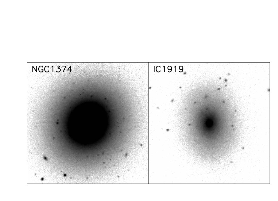
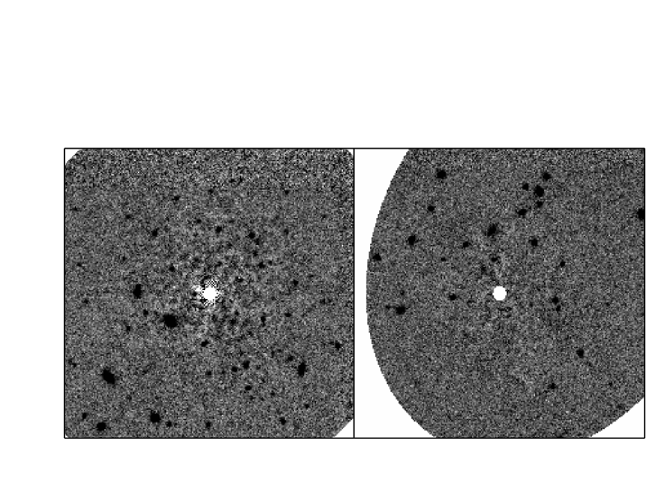

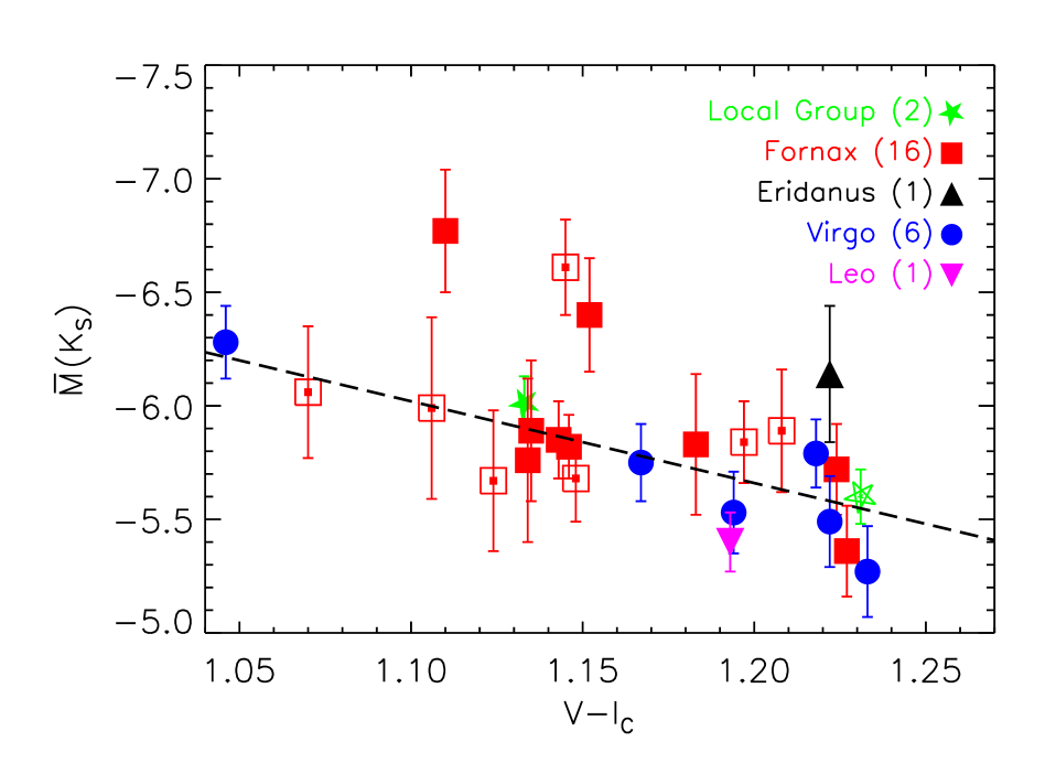


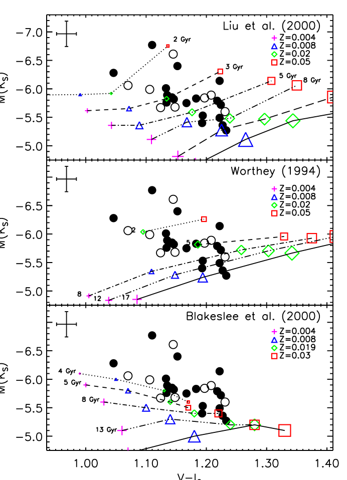
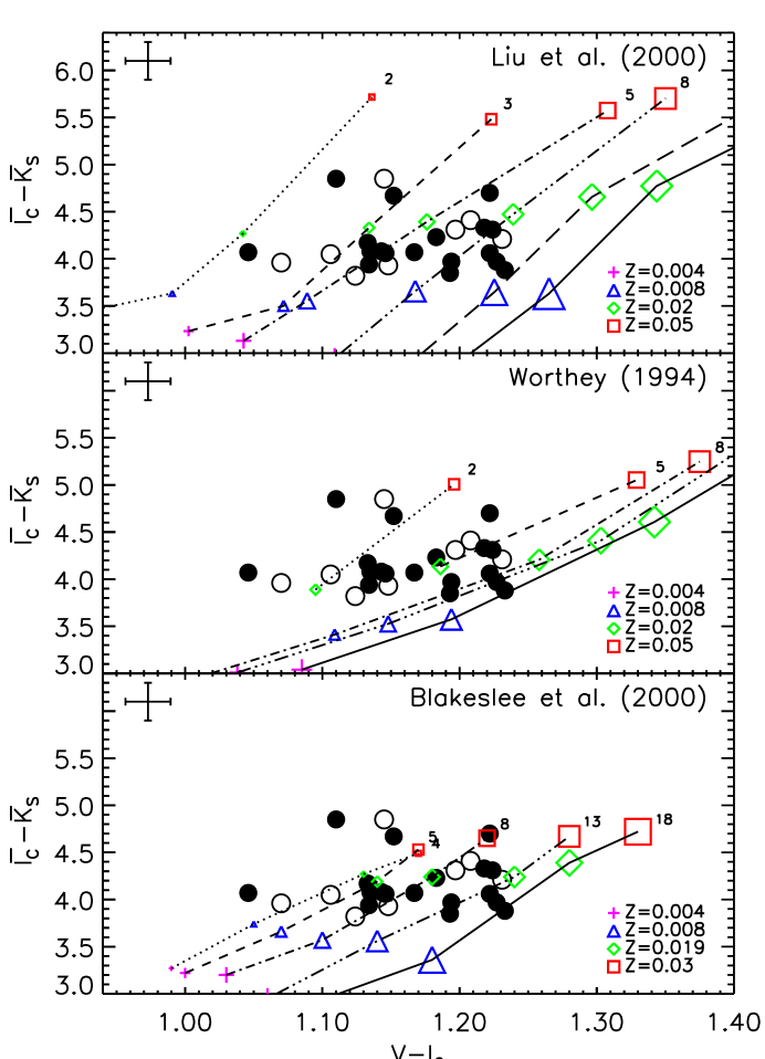
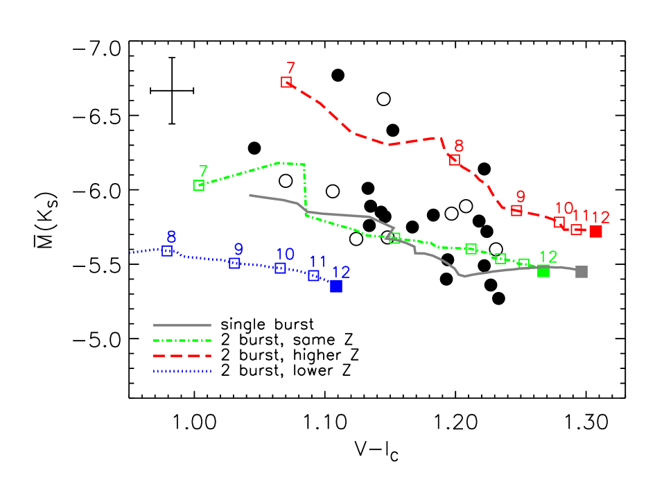
| Name | TypeaaFrom the NASA/IPAC Extragalactic Database (NED). | TbbFrom de Vaucouleurs et al. (1991) (RC3). | bbFrom de Vaucouleurs et al. (1991) (RC3). | Dia.aaFrom the NASA/IPAC Extragalactic Database (NED). | ccData are from Hypercat (http://www-obs.univ-lyon1.fr/hypercat), which uses an updated version of the literature compilation by Prugniel & Simien (1996). The exception is NGC 1373; its datum is from Graham et al. (1998). | ddFrom Schlegel et al. (1998). | eeFrom Tonry et al. (2000b). |
|---|---|---|---|---|---|---|---|
| (mag) | (arcmin) | (km s) | (mag) | (mag) | |||
| IC 1919 | SA(rs)0– | –3 | 13.80 | 1.6 1.2 | 26 | 0.06 | 1.108 0.018 |
| IC 2006 | E | –4 | 12.21 | 2.1 1.8 | 122 | 0.05 | 1.183 0.018 |
| NGC 1336 | SA0– | –3 | 13.10 | 2.1 1.5 | 115 | 0.05 | 1.124 0.032 |
| NGC 1339 | E4 | –4 | 12.51 | 1.9 1.4 | 171 | 0.06 | 1.134 0.012 |
| NGC 1344ffa.k.a. NGC 1340. | E5 | –5 | 11.27 | 6.0 3.5 | 159 | 0.08 | 1.135 0.011 |
| NGC 1351 | SA0– pec | –3 | 12.46 | 2.8 1.7 | 147 | 0.06 | 1.148 0.016 |
| NGC 1366 | S0 | –2 | 12.86 | 2.1 0.9 | 0.07 | 1.095 0.018 | |
| NGC 1373 | E | –4 | 14.12 | 1.1 0.9 | 79 | 0.06 | 1.085 0.013 |
| NGC 1374 | E | –4 | 12.00 | 2.5 2.3 | 207 | 0.06 | 1.146 0.016 |
| NGC 1375 | SAB0 | –2 | 13.18 | 2.2 0.9 | 69 | 0.06 | 1.070 0.019 |
| NGC 1379 | E | –5 | 11.80 | 2.4 2.3 | 130 | 0.05 | 1.143 0.019 |
| NGC 1380 | SA0 | –2 | 10.87 | 4.8 2.3 | 240 | 0.08 | 1.197 0.019 |
| NGC 1380Bgga.k.a. NGC 1382. | SAB(s)0– | –3 | 13.87 | 1.5 1.3 | 99 | 0.07 | 1.106 0.013 |
| NGC 1387 | SAB(s)0– | –3 | 11.68 | 2.8 2.8 | 0.06 | 1.208 0.047 | |
| NGC 1389 | SAB(s)0 | –3 | 12.42 | 2.3 1.4 | 0.05 | 1.145 0.019 | |
| NGC 1399 | E1 pec | –5 | 10.55 | 6.9 6.5 | 359 | 0.06 | 1.227 0.016 |
| NGC 1404 | E1 | –5 | 10.97 | 3.3 3.0 | 242 | 0.05 | 1.224 0.016 |
| NGC 1419 | E | –5 | 13.48 | 1.1 1.1 | 129 | 0.06 | 1.110 0.018 |
| NGC 1427 | E5 | –4 | 11.77 | 3.6 2.5 | 170 | 0.05 | 1.152 0.018 |
| Galaxy | ||||||
|---|---|---|---|---|---|---|
| (mag arcsec) | (mag) | (mag) | (mag) | (mag) | ||
| IC 1919 | 18.52 | 6.0 2.5 | 24.84 0.50 | 6.47 0.53 | 6.58 0.50 | 4.54 0.52 |
| IC 2006 | 17.77 | 4.7 0.3 | 25.76 0.11 | 5.83 0.31 | 5.66 0.14 | 4.23 0.29 |
| NGC 1336 | 18.49 | 2.9 0.4 | 25.71 0.23 | 5.67 0.31 | 5.71 0.25 | 3.82 0.28 |
| NGC 1339 | 17.57 | 4.3 0.4 | 25.85 0.08 | 5.76 0.36 | 5.57 0.12 | 3.94 0.36 |
| NGC 1344 | 17.21 | 18.6 0.9 | 25.59 0.10 | 5.89 0.31 | 5.83 0.12 | 4.08 0.31 |
| NGC 1351 | 17.60 | 5.4 0.6 | 25.93 0.11 | 5.68 0.19 | 5.48 0.13 | 3.93 0.17 |
| NGC 1366 | 19.00 | 2.2 0.6 | 25.51 0.43 | 6.11 0.52 | 5.91 0.43 | 4.12 0.51 |
| NGC 1373 | 18.56 | 9.0 1.9 | 25.11 0.37 | 6.67 0.60 | 6.31 0.38 | 4.63 0.59 |
| NGC 1374 | 17.05 | 8.3 0.3 | 25.66 0.05 | 5.82 0.14 | 5.75 0.09 | 4.06 0.11 |
| NGC 1375 | 17.82 | 10.6 1.2 | 25.52 0.26 | 6.06 0.29 | 5.90 0.27 | 3.96 0.28 |
| NGC 1379 | 17.08 | 12.0 0.9 | 25.66 0.08 | 5.85 0.17 | 5.75 0.12 | 4.08 0.14 |
| NGC 1380 | 16.28 | 7.4 0.5 | 25.39 0.04 | 5.84 0.18 | 6.02 0.09 | 4.31 0.15 |
| NGC 1380B | 17.95 | 5.3 0.4 | 25.78 0.25 | 5.99 0.40 | 5.63 0.27 | 4.05 0.39 |
| NGC 1387 | 17.28 | 8.2 0.7 | 25.65 0.06 | 5.89 0.27 | 5.77 0.10 | 4.41 0.15 |
| NGC 1389 | 17.53 | 14.0 0.8 | 25.07 0.10 | 6.61 0.21 | 6.35 0.13 | 4.85 0.19 |
| NGC 1399 | 16.01 | 5.2 0.5 | 26.14 0.12 | 5.36 0.20 | 5.28 0.15 | 3.97 0.18 |
| NGC 1404 | 16.67 | 8.9 0.6 | 25.89 0.05 | 5.72 0.20 | 5.53 0.10 | 4.31 0.17 |
| NGC 1419 | 17.92 | 16.6 1.4 | 24.65 0.13 | 6.77 0.27 | 6.77 0.15 | 4.85 0.26 |
| NGC 1427 | 17.51 | 9.5 0.5 | 25.46 0.06 | 6.40 0.25 | 5.96 0.10 | 4.67 0.23 |
Note. — The quantity measures the S/N of the stellar SBF signal (i.e., includes correction for unresolved contaminating point sources). The tabulated has been corrected for extinction. -band ’s were computed using two distance measurements to the galaxies: -band SBF distances to individual galaxies and a Cepheid distance to the cluster as a whole. The errors on the from the Cepheid group distance includes an allowance for the cluster’s rms depth but does not include the systematic error in the HST Cepheid zero point, estimated to be 0.16 mag (Mould et al., 2000a).
| Clusters | Distances | rms | ||||
|---|---|---|---|---|---|---|
| Fornax only | -band SBF (individual) | 5.81 0.06 | 14 | 0.23 | 1.0 | |
| 5.84 0.06 | 2.0 1.4 | 14 | 0.21 | 0.9 | ||
| Cepheid (cluster) | 5.74 0.03 | 14 | 0.20 | 2.8 | ||
| 5.78 0.04 | 4.1 1.6 | 14 | 0.22 | 2.5 | ||
| All galaxies | -band SBF (individual) | 5.76 0.04 | 24 | 0.28 | 2.1 | |
| 5.84 0.04 | 3.6 0.8 | 24 | 0.22 | 1.2 | ||
| Cepheid (cluster)aaDoes not include NGC 1407 in Eridanus since no Cepheid distance is available. | 5.68 0.03 | 23 | 0.25 | 4.2 | ||
| 5.75 0.03 | 4.3 0.7 | 23 | 0.23 | 2.4 |
Note. — Calibration of using only our Fornax results and our results combined with revised published data for Virgo, Leo, Eridanus, and Local Group galaxies. We either use -band SBF distances to individual galaxies or mean distances to the clusters from Cepheid distances in Ferrarese et al. (2000a). The linear fits are of the form , and the number of galaxies used for the fit is tabulated (). Also listed are the resulting rms (in mags) of the points after the fit and the reduced chi-square () . See § 5.1 for details.