A HEURISTIC INTRODUCTION TO RADIOASTRONOMICAL POLARIZATION

Abstract

Radio sources are often polarized. Accurate measurement of simply the flux density of a radio source requires a basic understanding of polarization and its measurement techniques. We provide an introductory, heuristic discussion of these matters with an emphasis on practical application and avoiding pitfalls.

Astronomy Department, University of California, Berkeley, CA 94720-3411; cheiles@astron.berkeley.edu

1. Introduction

Many astronomers wish nothing more than to measure the total flux density of a source. Radio sources are often polarized, so even this basic measurement requires a basic understanding of polarization. Astronomers whose vision is so limited should read §3.5. and 5.4., and then turn to some other activity.

Astronomers who are interested in astronomical magnetic fields and esoteric scattering geometries need to go further and measure polarization. Magnetic fields are a very important force in astrophysics, rivalling gravity and gas pressure in some regions such as interstellar space. Some extragalactic edge-on disks obscure light from the central black hole, but the highly polarized scattered light reveals not only the radiation from the black hole but also the properties of the scattering medium.

Synchrotron radiation is linearly polarized perpendicular to the magnetic field with fractional polarization typically $\sim 70\%$; pulsars are mainly linearly and partly circularly polarized; Faraday rotation, caused by the intervening magnetoionic gas, rotates the position angle of linear polarization; weak Zeeman splitting of spectral lines produces two circularly polarized components, and strong splitting also produces linear polarization; scattered spectral lines and continuum radiation are linearly, and sometimes weakly circularly, polarized.

The basic reference for our discussion of the fundamentals is the excellent book on astronomical polarization by Tinbergen (1996) and references therein. A more mathematical and fundamental reference is Hamaker, Bregman, and Sault (1996), which the theoretically-inclined reader will find of interest. Our discussion below will be heuristic in nature, avoiding proofs and mathematical detail. We will make several unproven statements and assertions; the explanations and justifications can be found in the abovementioned references. Practical details of calibration and application to real telescopes are in the series of Arecibo Observatory Technical and Operations Memos by Heiles and his collaborators and, also, in a forthcoming set of articles in the PASP; all of these are listed in the references.

2. The Jones vector for the electric field

2.1. Polarization of an oscillating telephone cord

It’s fun to take a long coiled telephone cord, tie one end to a fixed point, and wiggle the other end to excite standing waves. These waves are characterized by polarization, just as electromagnetic waves are.

If you wiggle back-and-forth vertically, it’s vertically linearly polarized, and ditto with horizontally. Let’s call these directions $X$ and $Y$, as in Figure 1a. (Contrary to usual, we denote the horizontal direction with $Y$!). More generally, define the position angle of polarization $\chi$ to be measured from the vertical in the counterclockwise direction; then when you wiggle at angle $\chi$, the position angle of linear polarization is also $\chi$. The peak amplitude in the $X$ direction is $A_{pX}=A_{p}\cos\chi$ and in the $Y$ direction $A_{pY}=A_{p}\sin\chi$. So generally, your wiggling produces amplitudes in both directions. Of course, the stronger you wiggle, the larger the amplitude $A_{p}$. So your wiggling in linear polarization mode can be specified by two quantities, the amplitude and the position angle.

Figure 1.: (a, left), linear polarization at position angle $\chi$; (b, right), $E_{45}$ is equivalent to the (non-vector) sum $(E_{X}+E_{Y})/\sqrt{2}$.

$\chi$ is periodic in $\pi$, not $2\pi$ like an ordinary angle. This means that linear polarization doesn’t have a direction; rather, it has an orientation. Often one represents its position angle on the sky by short lines, like iron filings. These lines are sometimes called vectors—incorrectly, because vectors do have a direction.

You can be fancier and wiggle with a circular motion, and this can be either clockwise or counterclockwise. This is circular polarization, and the two directions are called left-hand and right-hand circular. Here, too, you have amplitudes in both directions.

In what basic essence does the circular mode differ from the linear mode at $\chi=45\hbox{${}^{\circ}$}$? It’s not that the $X$ and $Y$ directions have different amplitudes. Rather, they have different phases. Specifically, suppose you describe your vertical wiggle with $A_{px}=A_{p}\cos(\omega t)$; then you’d describe the horizontal wiggle with $A_{pY}=A_{p}\sin(\omega t)$. One’s a cosine, the other a sine. Now, there is only one difference between a cosine and a sine: it’s the phase angle. Remember the trig identity

$$\sin(\omega t)=\cos\left(\omega t-{\pi\over 2}\right)$$ (1)

In other words, you can think of the $Y$ and $X$ amplitudes as being identical in all respects except that they differ in phase by $90^{\circ}$. The phase angle can be positive or negative: positive produces clockwise rotation, negative anticlockwise. More generally, the $X$ and $Y$ two amplitudes can differ in phase by an arbitrary angle $\phi$; when $\phi\neq 0^{\circ}$ or $90^{\circ}$, we have elliptical polarization. Elliptical polarization can also be described by different $X$ and $Y$ amplitudes.

2.2. Vectorial representation with trig notation for time

When you wiggle with linear polarization, you can describe $X$ and $Y$ amplitudes with identical trig functions, like $A_{Y}(t)=A_{pY}\cos(\omega t)$ and $A_{X}(t)=A_{pX}\cos(\omega t)$. It’s convenient to ignore the time dependence and write the peak amplitudes using vector notation:

$${\bf A_{p}}=\left[\begin{array}[]{c}A_{pX}\\ A_{pY}\end{array}\;\right]\;.$$ (4)

and in this case, with $A_{pX}=A_{p}\cos\chi$ and $A_{pY}=A_{p}\sin\chi$, we write

$${\bf A_{p}}=A_{p}\left[\begin{array}[]{c}\cos\chi\\ \sin\chi\end{array}\;\right]\;.$$ (7)

The meaning of this is perfectly clear without explicitly writing the time dependence. However, suppose we are dealing with circular polarization. Then, with ordinary trig notation, we need to explicitly include the time dependence and write

$${\bf A(t)}=\left[\begin{array}[]{c}A_{pX}\cos(\omega t)\\ A_{pY}\cos(\omega t+\phi)\end{array}\;\right]\;.$$ (10)

which is awkward: our description of the wiggling doesn’t really need the time dependence, which only specifies in a cumbersome way that the motion is periodic with a certain frequency. What’s really important is the phase angle. To reflect this, often an equation like the above is simplified by writing

$${\bf A_{p}}=\left[\begin{array}[]{c}A_{pX}\\ A_{pY}\angle\phi)\end{array}\;\right]\;.$$ (13)

The meaning of this is clear, but mathematically one can’t manipulate the angle sign so it isn’t useful in a mathematical sense.

2.3. Complex exponential notation

Complex exponential notation is handy because it eliminates the need to explicitly write the time dependence in terms of $(\omega t)$, it allows one to specify phase angles, and the notation can be mathematically manipulated. We recall that the complex plane has a real and imaginary axis. The cosine and sine functions are the projections of a complex exponential on the real and imaginary axis, respectively. We have

$$e^{i\theta}=\cos\theta+i\sin\theta$$ (14)

which leads to

$$\cos\theta=Re\ [e^{i\theta}]$$ (15)

$$\sin\theta=Im\ [e^{i\theta}]=Re\ [-ie^{i\theta}]$$ (16)

and, most importantly it allows the addition of a phase angle to be replaced by the multiplication of its complex exponential,

$$\cos(\theta+\phi)=Re\ [e^{i(\theta+\phi)}]=Re\ [e^{i\theta}e^{i\phi}]$$ (17)

$$\sin(\theta+\phi)=Re\ [-ie^{i(\theta+\phi)}]=Re\ [-ie^{i\theta}e^{i\phi}]$$ (18)

This last is important for our purposes because we can use exponential notation to replace equation 10 with

$${\bf A}=\left[\begin{array}[]{c}A_{pX}\\ A_{pY}e^{i\phi}\end{array}\;\right]\;,$$ (21)

which tells the essence, namely that $A_{Y}$ lags $A_{X}$ by phase $\phi$.

All aspects of the above discussion carry over to the electric field in electromagnetic waves; we simply replace the amplitude $A$ with the electric field $E$. Its vector representation is called the Jones vector.

3. Polarized power and the Stokes vector

In astronomy we are almost never interested in the electric field because we measure the power. Power is the time average of the square of the electric field. Or, rather, the time average of the product of the electric field with its complex conjugate; this takes care of any difficulties with phases.

3.1. How many parameters are required?

We made a heuristic argument above that the polarization is specified by three parameters, namely the three in equation 21. However, there is one additional wrinkle. We were describing a $100\%$ polarized wave in which the amplitude has a single frequency and, correspondingly, a single polarization mode, which is generally elliptical. Any monochromatic wave exists forever, so its polarization never changes.

However, there can also exist a superposition of sine waves of different frequencies within some bandwidth. In fact, this is always the case of natural radiation like sunlight, the 21-cm line, or even astronomical masers. In nature, they are packed tightly together in frequency with infinitely small separations. They produce an electric field that varies randomly with time. These fields can all be polarized in the same sense, just like a monochromatic wave.

But the polarizations can also be randomly distributed with frequency. In this case we have unpolarized radiation. The Jones vector, which treats a single sine wave and has only three parameters, is not adequate to describe this case.

This extra possibility, that the electric field can have a time-random unpolarized component, turns the three parameters into four: the fourth tells the fraction of power that is nonpolarized. These four parameters are combinations of polarized power called Stokes parameters.

Stokes parameters are linear combinations of power measured in orthogonal polarizations. We measure power in a particular polarization by constructing an antenna that responds to that polarization, meaning that the incoming electric field generates a corresponding voltage in a cable. With a radio astronomy “dish”, the antenna is called a feed. Here we will think of a feed’s antenna as a probe in a waveguide that extracts linear polarization. More generally, feeds can be made to sample linear, circular, or even arbitrary elliptical polarization.

We describe radiation in terms of electric fields having particular polarizations; what we mean is that we have constructed an antenna sensitive to that polarization and when we write the electric field $E$ we really mean voltage in the cable that was induced by the field.

3.2. Linear polarization: Stokes Q and U

It’s intuitively obvious that orthogonal linear polarizations have $\chi$ differing by $90^{\circ}$: for example, vertical ($X$) and horizontal ($Y$) polarizations are orthogonal and have $\chi=(0^{\circ},90^{\circ})$, respectively.

The power in the $(X,Y)$ directions is just $(E_{X}^{2},E_{Y}^{2})$, respectively. We can linearly combine these two powers by adding and subtracting them, and in the process we generate the first two Stokes parameters $I$ and $Q$:

$$I=E_{X}^{2}+E_{Y}^{2}=E_{0^{\circ}}^{2}+E_{90^{\circ}}^{2}$$ (22)

$$Q=E_{X}^{2}-E_{Y}^{2}=E_{0^{\circ}}^{2}-E_{90^{\circ}}^{2}$$ (23)

Let us reflect on these quantities for a moment.

The sum: Stokes I

The sum represents the total power in the incoming radiation. It makes intuitive sense that, by sampling two orthogonal polarizations, you pick up all of the incoming power. It may not make intuitive sense, but is nevertheless true, that it doesn’t matter which two orthogonal polarizations you measure and add together. The orthogonal circulars, or two orthogonal linears at any pair of angles $(\chi,\chi+90^{\circ})$, or even orthogonal ellipticals always sample all of the power and their summed powers always gives the total intensity $I$.

This is easy to see for the particular case of linear polarization at $\chi=45^{\circ}$. You can express $E_{0^{\circ}}$ in terms of $(E_{45^{\circ}},E_{-45^{\circ}})$ (see Figure 1b):

$$E_{0^{\circ}}={E_{45^{\circ}}+E_{-45^{\circ}}\over\sqrt{2}}$$ (24)

$$E_{90^{\circ}}={E_{45^{\circ}}-E_{-45^{\circ}}\over\sqrt{2}}$$ (25)

and when you take the sum of the squares, you find—naturally enough—that $E_{0^{\circ}}^{2}+E_{90^{\circ}}^{2}=E_{45^{\circ}}^{2}+E_{-45^{\circ}}^{2}$.

The difference: Stokes Q

The difference tells about the polarization. Suppose the incoming electric field is vertically polarized (the $X$ direction); then $Q=I$. If it’s horizontally polarized, then equation 23 says $Q=-I$. If it’s coming in at $\chi=45^{\circ}$, then $Q=0$. In fact, more generally,

$${Q\over I}=p_{QU}\ \cos(2\chi)$$ (26)

where $p_{QU}$ is the total fractional linear polarization (which we discuss below). So $Q$ is a very valuable diagnostic of the linear polarization! But also it’s not complete: for example, for $\chi=45^{\circ}$ we have $Q=0$ and, with this parameter alone, we would not suspect that the signal is polarized.

Another difference: Stokes U

We need one more parameter to completely define the linear polarization. That parameter is Stokes $U$, and is equal to

$$U=E_{45^{\circ}}^{2}-E_{-45^{\circ}}^{2}$$ (27)

With a little reflection it becomes clear that

$${U\over I}=p_{QU}\ \sin(2\chi)$$ (28)

The combination $(Q,U)$ completely specifies the linear polarization of the signal. The combination $(Q^{2}+U^{2})^{1/2}$ is the total linearly polarized power and is independent of $\chi$. Generally, even for a partially polarized signal, the fraction of linear polarization and its position angle are given by

$$p_{QU}=\left[\left({Q\over I}\right)^{2}+\left({U\over I}\right)^{2}\right]^{1/2}$$ (29)

$$\chi=0.5\tan^{-1}{U\over Q}$$ (30)

3.3. Circular polarization: Stokes V

There are only two circular polarizations, which are called right- and left-handed, or RCP and LCP, and they are orthogonal. So one can derive two Stokes parameters from them: one is $I$, which is the same as discussed above; you can include the $90^{\circ}$ phase difference in equations such as 24 and 25 prove this for yourself.

The difference is Stokes $V$. If you ever work with circular polarization, you have to be careful about sign. Physicists use one definition, radio astronomers use another (the IEEE definition, reflecting our EE heritage), and optical astronomers use both, sometimes without bothering to specify exactly which they are using. The IEEE definition is

$$V=E_{LCP}^{2}-E_{RCP}^{2}$$ (31)

$LCP$ is generated by transmitting with a left-handed helix, so from the transmitter the E vector appears to rotate anticlockwise. From the receiver, $LCP$ appears to be rotating clockwise.

We define the fractional circular polarization just as we do for linear polarization:

$$p_{V}={V\over I}$$ (32)

$V$ can be positive or negative, and one can retain the sign in the definition of $p_{V}$ if one wishes, as we’ve done here.

3.4. The Stokes vector and total polarized power

We have four Stokes parameters, and it will be convenient to write them in vector format, the 4-element Stokes vector

$${\bf S}=\left[\begin{array}[]{c}I\\ Q\\ U\\ V\\ \end{array}\;\right]\;.$$ (37)

The total fractional polarization is just

$$p=\left[\left({Q\over I}\right)^{2}+\left({U\over I}\right)^{2}+\left({V\over I}\right)^{2}\right]^{1/2}$$ (38)

If both $p_{QU}$ and $p_{V}$ are nonzero, then the polarization is elliptical, which is the general situation. Every elliptical polarization has its orthogonal counterpart, and one can even build an elliptically polarized feed. One normally prefers pure linear or circular and tries to avoid the intermediate cases. However, Arecibo uses turnstile junctions for some receivers, which have the advantage that the polarization can be adjusted to pure circular with exquisite accuracy—but the polarization becomes increasingly elliptical, changing to linear and back again, with increasing departure from the design frequency (see Heiles et al 2000b, 2001b)!

3.5. If you don’t remember anything else, remember THIS!

Often you find yourself needing to combine polarizations. For example, if you measure the polarization of some object several times, you need to average the results.

There is only one proper way to combine polarizations, and that is to use the Stokes parameters. The reason is simple: because of conservation of energy, powers add and subtract. But it is definitely wrong to average fractional polarizations or angles. Consider that fractional polarizations are always positive, so they can never average to zero. And angles are even worse! Consider averaging two measurements having angles of $0\hbox{${}^{\circ}$}$ and $179\hbox{${}^{\circ}$}$—angles that differ by only $1\hbox{${}^{\circ}$}$ because of the $\pi$ periodicity of position angle. The straight average of the angles gives about $90\hbox{${}^{\circ}$}$—the orthogonal polarization!

What you must do is convert the fractional polarization and position angle to Stokes parameters, average the Stokes parameters, and convert back to fractional polarization and position angle.

4. Measuring Stokes parameters in radio astronomy

In contrast to optical astronomers, radio astronomers can measure all Stokes parameters simultaneously. It may not be obvious how they do this: we’ve described Stokes parameters as differences between powers in various pairs of orthogonal polarizations, each pair “belonging” to a particular Stokes parameter, and we can’t simultaneously place six feed probes at the same physical location to simultaneously measure $(E_{0^{\circ}},E_{90^{\circ}},E_{45^{\circ}},E_{-45^{\circ}},E_{LCP},E_{RCP})$ because all these antennas would interact with other and make a total mess. Fortunately, we can generate a Stokes parameter not only by subtraction of its own orthogonal polarizations, but also by multiplying electric fields of two orthogonal polarizations belonging to a different Stokes parameter.

4.1. Example: generating Stokes U from $(E_{0^{\circ}},E_{90^{\circ}})$

This is easy to see for the case of deriving Stokes $U$ (which is $E_{45^{\circ}}^{2}-E_{-45^{\circ}}^{2}$) from it’s non-belonging brethren $(E_{0^{\circ}},E_{90^{\circ}})$. Referring again to Figure 1b, it is clear, graphically speaking, that the product $(E_{0^{\circ}}E_{90^{\circ}})$ is related to Stokes $U$. As the E field at $\chi=45^{\circ}$, which belongs to Stokes $U$, oscillates, it induces in-phase fields in the $0^{\circ},90^{\circ}$ directions, each smaller by a factor of $\sqrt{2}$. The E-fields in these two directions are therefore correlated. If you measure the time average product $\langle E_{0^{\circ}}E_{90^{\circ}}\rangle$, it’s identical to $\langle E_{45^{\circ}}^{2}\rangle\over 2$.

In particular, if you begin with equations 24 and 25 you can easily show that

$$U\equiv E_{45^{\circ}}^{2}-E_{-45^{\circ}}^{2}=2E_{0^{\circ}}E_{90^{\circ}}$$ (39)

If you throw in a phase factor of $90^{\circ}$ in the above equation, you’ll recover Stokes $V$—this makes sense because the only difference between linear and circular polarization is, in fact, the phase factor.

4.2. A general expression for Stokes parameters

One can write Stokes parameters in terms of electric fields of any two orthogonal polarizations. Here we provide the version in which one measures $(E_{X},E_{Y})$ with linearly polarized antennas at $\chi=0^{\circ}$. For this case,

$$I=E_{X}\overline{E_{X}}+E_{Y}\overline{E_{Y}}$$ (40)

$$Q=E_{X}\overline{E_{X}}-E_{Y}\overline{E_{Y}}$$ (41)

$$U=E_{X}\overline{E_{Y}}+\overline{E_{X}}E_{Y}$$ (42)

$$iV=E_{X}\overline{E_{Y}}-\overline{E_{X}}E_{Y}\;.$$ (43)

The overbar indicates the complex conjugate. These products are time averages; we have omitted the indicative $\langle\rangle$ brackets to avoid clutter. And remember, these equations apply to the voltages induced into the antenna as well as to the original electric fields, because they are proportional; below, we are always referring to voltages even though we will write $E$.

These equations make it clear how to measure all four Stokes parameters simultaneously. Namely, begin with orthogonal polarizations; any pair will do, but our equations are written for orthogonal linears. Then digitize the resulting voltages and perform the above products in a computer. The aspects of digitizing and computing are a story all in themselves, but we leave that for another time.

4.3. The need for calibration

The above equations 40-43 are simple in theory but not so simple in practice because the radioastronomical receiving system produces unwanted modifications in the astronomical polarization. Feeds are almost never perfect, so their polarizations are only approximately linear or circular; and generally speaking, no feed has two outputs that are perfectly orthogonal.

Figure 2.: Two versions of a radio astronomical receiver: (a,left), good; (b, right), bad (see §5.3. and 5.4.).

Most important in practice is the electronics system, which introduces its own relative gain and phase differences between the two linearly polarized channels. Figure 2a shows the important elements of the system for this discussion. Two orthogonal feed probes in a waveguide convert the incoming electric field to voltages. These travel through cables having lengths $(L_{X},L_{Y})$ to a directional coupler, where the correlated noise source is injected (through cables of different length—a fact we ignore for the sake of simplicity). $(L_{X},L_{Y})$ cannot be exactly identical, and the difference produces a phase shift between the two polarization channels. The two polarization channels are amplified with gains that are inherently complex, meaning that each introduces its own phase shift. The signals are multiplied in a mixer by a local oscillator, again injected through cables whose lengths cannot be precisely equal, leading to an additional phase offset between the channels. The resulting i.f. signals are sent down to the digital correlator through cables from the feed; these also have different lengths and losses.

The total gains in the (left, right) channels are $(G_{X}G_{A},G_{Y}G_{B})$. If the magnitudes of these gains differ, then the difference between the two channels is nonzero for an unpolarized source, making the source appear to be linearly polarized. If the phases differ, then a linearly polarized source appears to be circularly polarized. These electronics gains and phases must be calibrated relatively frequently because they can change with time. This calibration is most effectively done by injection of a correlated noise source into the two feed outputs.

5. Calibration: Jones and Mueller matrices

The modification of the derived polarization by the system components is most generally described by matrices. The Jones matrix describes the modification of the Jones vector, and the Mueller matrix describes the modification of the Stokes vector.

Return to our wiggling telephone cord. Suppose we wiggle one end with linear polarization in the vertical direction, making $Q=I$ and $(U,V)=0$. Now a Martian spy starts to move the other end around in a small circle at the same frequency. This would change the original pure vertical linear polarization into elliptical polarization, taking some power from $Q$ and putting it into $U$ and $V$.

Feeds and electronic devices are like the Martian, modifying the electric field’s polarization. Generally, a device can couple an arbitrary fraction of the $Y$ voltage into $X$ with an arbitrary phase; and also vice-versa. The easy way to write these mutual perturbations is with a matrix transfer function that relates the output voltages to the input voltages. This matrix operates on the Jones vector, so it is naturally called the Jones matrix. With two orthogonal polarizations, there are two voltages; thus the Jones matrix is $2\times 2$.

If the Jones matrix is unitary, then it produces no modification in the original polarization. Unitary matrices aren’t very interesting in astronomy, because we need lots of amplification for the tiny voltages induced at the feed! But we can imagine a system in which the Jones matrix is diagonal; that would mean there is no coupling between the $X$ and $Y$ channels. Large diagonal elements would increase the voltages so that we can measure them, and if the two diagonal elements were equal, it would also keep the polarization—and thus the Stokes parameters—unchanged.

More generally, the Jones-matrix-modified voltages change the polarization state, and thus change the Stokes parameters. So every Jones matrix has its Stokes-parameter counterpart, which is called the Mueller matrix. The Mueller matrix relates the output Stokes vector of equation 37 to the input Stokes vector:

$${\bf S_{out}}={\bf M\cdot S_{in}}\;.$$ (44)

There are four Stokes parameters, so the Mueller matrix is $4\times 4$; in general, all elements may be nonzero, but they are not all independent. In the usual way, we write

$${\bf M}=\left[\begin{array}[]{cccc}m_{II}&m_{IQ}&m_{IU}&m_{IV}\\ m_{QI}&m_{QQ}&m_{QU}&m_{QV}\\ m_{UI}&m_{UQ}&m_{UU}&m_{UV}\\ m_{VI}&m_{VQ}&m_{VU}&m_{VV}\\ \end{array}\;\right]\;.$$ (49)

Each matrix parameter is the coupling of the two Stokes parameters indicated by its subscripts.

Each system component has its own Jones and Mueller matrices, and the total system matrices are the products of the individual component’s matrices. The Mueller matrix for the feed has complicated off-diagonal elements. Fortunately, feeds are usually well-designed and these off-diagonal elements are small, meaning the instrumental polarization is small.

Here, we will restrict our detailed discussion to the two most important specific components, the electronics chain and the coupling of the telescope to the sky; fortunately they are also the simplest. For a complete treatment that includes the feed, see Heiles et al (2000a, 2000b).

5.1. The Jones and Mueller matrices for the electronics chain

The two polarization channels go through different amplifier chains as in figure 2a, and we can safely assume that there is no coupling between the channels in the electronics system; this, in turn, means that the nondiagonal elements of the Jones matrix are zero. Suppose the two channels have voltage gain $(g_{A},g_{B})$, power gain $(G_{A},G_{B})=(g_{A}^{2},g_{B}^{2})$, and phase delays $(\psi_{A},\psi_{B})$. Clearly, the Jones matrix is

$$\left[\begin{array}[]{c}E_{A,out}\\ E_{B,out}\\ \end{array}\;\right]=\left[\begin{array}[]{cc}g_{A}e^{i\psi_{A}}&0\\ 0&g_{B}e^{i\psi_{B}}\\ \end{array}\;\right]\left[\begin{array}[]{c}E_{A,in}\\ E_{B,in}\\ \end{array}\;\right]\;$$ (56)

You calculate the Mueller matrix $\bf M_{A}$ from the Jones matrix by the laborious procedure of applying equations 40-43. The result is surprisingly complicated. However, for a well-designed and calibrated system, we can assume that the two gains $(g_{A},g_{B})$ are nearly identical, and for simplicity assume that their average is unity. That is, we can assume that

$$\Delta G\equiv G_{A}-G_{B}\ll 1$$ (57)

We then carry the algebra only to first order in $g_{A}g_{B}$, meaning we take $g_{A}g_{B}=1$. With this first-order approximation, the electronics Mueller matrix becomes

$${\bf M_{A}}=\left[\begin{array}[]{cccc}1&{\Delta G\over 2}&0&0\\ {\Delta G\over 2}&1&0&0\\ 0&0&\cos\psi&-\sin\psi\\ 0&0&\sin\psi&\cos\psi\\ \end{array}\;\right]\;.$$ (62)

Here we have set $\psi\equiv\psi_{A}-\psi_{B}$: the difference is all that matters because it’s always the relative phase between the two channels that counts. The matrix consists of two submatrices, the upper left and the lower right. Let’s reflect on these submatrices.

The upper left submatrix represents coupling between Stokes $I$ and $Q$. The relative gain error directly affects these two parameters because they are the sum and difference of the $X$ and $Y$ powers. In contrast, these powers are completely unaffected by the phase difference, so $\psi$ doesn’t appear in this submatrix. The two diagonal elements are unity because we’ve assumed $\Delta G\ll 1$. Consider the specific example of an unpolarized source: a gain difference makes it look polarized, with $Q$ nonzero, and it also affects Stokes $I$.

The lower right submatrix represents coupling between Stokes $U$ and $V$. The relative phase directly affects these two parameters because they are the correlated products $E_{X}E_{Y}$, and the departure of the correlation’s phase angle from zero directly reflects the degree of circular polarization, Stokes $V$.

5.2. A very important property of correlated voltages

Embodied in equation 62 is a highly important principle: gain errors do not affect correlation products when there is no polarization. This is important because amplifier gains fluctuate with time and their calibration is subject to measurement error; in contrast, amplifier phase delays and cable lengths tend to change only slowly with time.

Consider the case of a nonpolarized source. Equation 62 shows that the error in the measured Stokes $Q$ is directly proportional to $\Delta G$. However, Stokes $U$ and $V$ are completely independent of $\Delta G$, so a nonpolarized source cannot produce fake nonzero $(U,V)$. This is because if $E_{X}E_{Y}=0$, as it is for an unpolarized source, then the product is zero even with a gain error.

In practice, this makes the measurement of small polarizations more accurate when using correlated products. This fundamental fact appears again and again in precision radioastronomical measurements of small quantities, and is also the basis for interferometry. The corollary is the somewhat nonintuitive fact: If you want to measure small circular polarizations accurately, then use linearly polarized feeds; if you want to measure small linear polarizations accurately, then use circularly polarized feeds!

5.3. Carrying correlation too far: using a hybrid

Suppose you want to measure weak linear polarization. As we discussed above, the best technique is to crosscorrelate orthogonal circulars. But suppose your telescope only has a linearly polarized feed!

You may be tempted to modify the system block diagram to include a $90\hbox{${}^{\circ}$}$ hybrid, as shown in Figure 2b. The hybrid inserts a $90\hbox{${}^{\circ}$}$ phase shift into one channel and then adds them. This turns the dual linear system [polarizations $(X,Y)$] into a dual circular one [polarizations $(A,B$)]. You can then use the crosscorrelation technique to generate the dual linears.

However, this system does not provide the abovementioned advantage of crosscorrelation in measuring small signals. The reason is simple: the $(X,Y)$ signals are combined after the first amplifier and have been multiplied by the gains $(G_{X},G_{Y})$ with their corresponding uncertainty and time variability. Thus, the combined $(A,B)$ signals are pure circular polarization only to the extent that $G_{X}=G_{Y}$—and, of course, this includes their complex portions, the phases, as well. And we are ignoring the inevitable imperfections in the hybrid. After the hybrid, the complex channel gains $(G_{A},G_{B})$ operate on the signal, as usual.

We now have four combinations of gain to worry about: $(G_{X}G_{A},G_{X}G_{B}$, $G_{Y}G_{A},G_{Y}G_{B})$. In contrast, the straightforward system without the hybrid has only two combinations: $(G_{X}G_{A},G_{Y}G_{B})$. This makes the calibration process for the hybrid system more complicated, requiring turning on the correlated cal not only when it is connected to both channels simultaneously but also when it is connected to each one individually, one at a time. The details are discussed by Heiles and Fisher (1999).

The hybrid completely removes the cross correlation advantage: with the hybrid, there is no Stokes parameter that is unaffected by $\Delta G$.

5.4. Stokes I and the hybrid

The hybrid even creates problems measuring Stokes $I$ because of the more complicated calibration procedure described above. Unfortunately, however, astronomers rather traditionally prefer to measure Stokes $I$ using dual circular polarization instead of dual linear. The reason is partly scientific, partly historical. Historically, the first receiving systems had only a single polarization channel: it was hard and expensive enough to make a single low-noise receiver, let alone two. Classical radio sources, such as quasars, often exhibit significant linear polarization, but very little circular. Thus, to obtain reliable, repeatable flux density measurements—particularly at low frequency, where ionospheric Faraday rotation is important—the single polarization of choice was circular. Similarly, in historic single-polarization VLBI with its differing ionospheric Faraday rotations at the different stations, circular polarization was preferred. And finally, pulsars are more highly linearly than circularly polarized. When faced with a single polarization system and sources that are linearly polarized, the polarization of choice is circular because one needs only to multiply the measured flux by two to get Stokes $I$.

This traditional emphasis on circular polarization persists in dual-polarized receivers. Many astronomers who want to measure nothing more than Stokes $I$, when faced with a dual-linear system, insert a hybrid to convert the system to dual-circular. But they don’t carry through with the extra steps of calibration required.

To bring the point home that using a hybrid is inappropriate, consider the extreme case when the $Y$-polarization amplifier is turned off. The astronomer who uses a hybrid points the telescope to the source of interest and sees both channels $(A,B)$ respond. Then he turns on the cal and sees both channels respond. He has no idea that one channel is dead. He might wonder why the levels are 3 db lower than usual, but astronomers usually don’t pay attention to power levels, ascribing them to the domain of the receiver engineer.

In historical times, radio astronomers often did use a hybrid to generate the circular polarization(s) from a dual linear feed, but placed the hybrid before the first amplifier. This is far better, because then one is reduced to the simpler situation of having only two sets of gains to determine, $(G_{X}G_{A},G_{Y}G_{B})$. The problem with this approach is that hybrids have some loss, and therefore introduce noise. In those historical times receiver temperatures were high enough that this extra noise could be tolerated. Today’s receiver temperatures are too low for this approach unless the hybrid is cooled.

The moral: don’t ever use a post-amp hybrid unless you really need to change the polarization for a special, specific purpose! To measure Stokes $I$, use the native feed polarization; calibrate and measure the two polarization channels independently, and add the results.

5.5. The Mueller matrix for the sky

A linearly polarized astronomical source has Stokes $(Q_{src},U_{src})$ parameters defined with respect to the north celestial pole (NCP). It’s these quantities that we want to measure.

The first device encountered by the incoming radiation is the telescope (${\bf M_{SKY}}$). These days, all major telescopes are alt-az mounted,. This means that the feed mechanically rotates with respect to the sky as the dish tracks the source. The angle of rotation is called the parallactic angle $PA_{az}$. It is defined to be zero at azimuth $0\hbox{${}^{\circ}$}$ and increase towards the east; for a source near zenith, which is always the case at Arecibo, $PA_{az}\sim az$, where $az$ is the azimuth angle of the source. The Stokes parameters seen by the feed are $(Q_{sky},U_{sky})$; the conversion between ${\bf S_{src}}$ and ${\bf S_{sky}}$ is given by the Mueller matrix

$${\bf M_{SKY}}=\left[\begin{array}[]{cccc}1&0&0&0\\ 0&\cos 2PA_{az}&\sin 2PA_{az}&0\\ 0&-\sin 2PA_{az}&\cos 2PA_{az}&0\\ 0&0&0&1\\ \end{array}\;\right]\;.$$ (67)

The central $2\times 2$ submatrix is, of course, nothing but a rotation matrix. $\bf M_{SKY}$ doesn’t change $I$ or $V$, which makes sense.

For an equatorially-mounted telescope, the feed doesn’t rotate on the sky as the source is tracked. This fact might still be of interest to optical astronomers, but with the demise of the last of the great equatorial telescopes—the NRAO 140-footer—this fact recedes into the fog of history for us radio astronomers.

5.6. The total system Mueller matrix

Heiles et al (2000a, 2001a) define seven parameters that specify the complete system Mueller matrix. Two of these refer to the cal gain and phase with respect to the sky (equation 62 above), four refer to the ellipticity and nonorthogonality of the feed, and the seventh is a rotation angle. In contrast, the $4\times 4$ Mueller matrix contains sixteen elements; not all of the elements are independent. For illustrative purposes, we write the full system matrix, without the sky correction, in terms of the first six parameters:

$$\left[\begin{array}[]{cccc}1&(-2\epsilon\sin\phi\sin 2\alpha+{\Delta G\over 2}\cos 2\alpha)&2\epsilon\cos\phi&(2\epsilon\sin\phi\cos 2\alpha+{\Delta G\over 2}\sin 2\alpha)\\ {\Delta G\over 2}&\cos 2\alpha&0&\sin 2\alpha\\ 2\epsilon\cos(\phi+\psi)&\sin 2\alpha\sin\psi&\cos\psi&-\cos 2\alpha\sin\psi\\ 2\epsilon\sin(\phi+\psi)&-\sin 2\alpha\cos\psi&\sin\psi&\cos 2\alpha\cos\psi\end{array}\;\right]$$

$\Delta G$ is the error in relative intensity calibration of the two polarization channels. It results from an error in the relative cal values $(T_{calA},T_{calB})$.

$\psi$ is the phase difference between the cal and the incoming radiation from the sky (equivalent in spirit to $L_{X}-L_{Y}$ on our block diagram..

$\alpha$ is a measure of the voltage ratio of the polarization ellipse produced when the feed observes pure linear polarization.

$\chi$ is the relative phase of the two voltages specified by $\alpha$.

$\epsilon$ is a measure of imperfection of the feed in producing nonorthogonal polarizations (false correlations) in the two correlated outputs.

$\phi$ is the phase angle at which the voltage coupling $\epsilon$ occurs. It works with $\epsilon$ to couple $I$ with $(Q,U,V)$.

$\theta_{astron}$ is the angle by which the derived position angles must be rotated to conform with the conventional astronomical definition.

6. Calibrating and using the matrix parameters

6.1. The role of the correlated cal

In practice, the amplifier gains and phases are calibrated with a correlated noise source (the “cal”). Thus, our amplifier gains $(G_{A},G_{B})$ in equation 62 have nothing to do with the actual amplifier gains. Rather, they represent the gains as calibrated by specified cal intensities, one for each channel. If the sum of the specified cal intensities is perfectly correct, then the absolute intensity calibration of the instrument is correct for an unpolarized source (i.e. Stokes $I$ is correctly measured in absolute units). Above, we have assumed $G_{A}+G_{B}=2$, which means that we are dealing with fractional polarizations and neglecting the absolute calibration of intensity.

The difference between the amplifier phases is also referred to the cal. Thus the phase difference $\psi=\psi_{A}-\psi_{B}$ represents the phase difference that exists between a linearly polarized astronomical source and the cal and has nothing to do with the amplifier chains.

We assume the cal to be constant. Thus, the measured Stokes vector is referred to the cal. This means that all artifacts of the electronics chain, which change with time, are removed by referring the measured Stokes vector to the cal, which is constant in time.

It remains to relate the cal to the sky. This must be done by astronomical observations that determine the Mueller matrix of the calibrated system. In other words, the calibrated system’s Mueller matrix multiplies the incoming Stokes vector from the sky and produces the measured Stokes vector.

6.2. Determining the Mueller matrix astronomically

Astronomical radio sources exhibit signficant linear polarization but usually negligible circular polarization. We determine the matrix astronomically by tracking a linearly polarized radio source over a wide range of parallactic angle $PA$. As $PA$ changes, Stokes $Q$ and $U$ from the source are modified by ${\bf M_{SKY}}$ in equation 67. In contrast, any $PA$ dependence of the measured Stokes $V$ must reveal nonzero matrix elements coupling Stokes $(Q,U)$ into $V$, namely $(m_{QV},m_{UV})$ and their two counterparts.

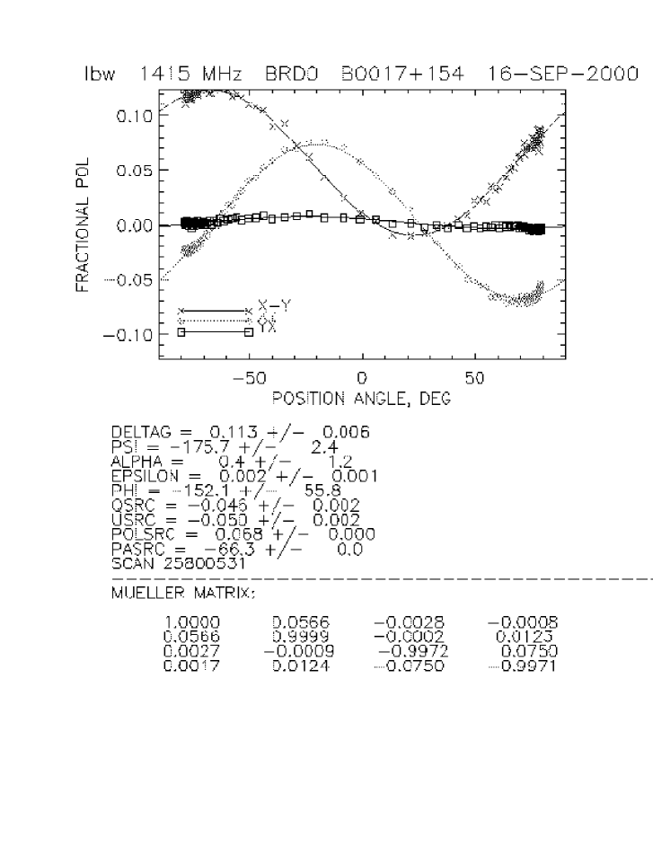
Figure 3.: A calibration observation of the source $0017+154$ for Arecibo’s dual-linear LBW feed. At the top, the measured Stokes parameters, uncorrected for the system’s and sky Mueller matrices, versus $PA$. In the middle and bottom we have the derived values for the instrumental parameters for the total Mueller matrix, and also the Mueller matrix itself (§mmsystem).

Figure 3 shows a calibration observation vfor Arecibo’s dual-linear LBW feed. The crosses show the $PA$ dependence of $X-Y$—the difference between the two linears, which is the measured Stokes $Q$; the diamonds show $XY$, the measured Stokes $U$. They follow sine and cosine waves with comparable amplitudes, as they should (equations 26, 28). The smallness of the departure from these conditions is expressed by the tiny values for $(m_{QU},m_{UQ})$. The amplitude of the sine/cosine curves gives the linear polarization of the source, $\sim 7\%$.

However, the sine wave for the crosses is displaced above zero by about 0.06. This reflects coupling of Stokes $I$ into $Q$, $m_{QI}$; this is the effect of nonzero $\Delta G$, an error in the relative cal values. In contrast, $m_{UI}$ is very small, consistent with its derivation from crosscorrelation; the fact that $m_{UI}\neq 0$ reflects cross coupling in the feed, which is described by the parameter $\epsilon$ above.

Finally, Stokes $V$ exhibits a small $PA$ dependence, which indicates nonzero values for $(m_{UV},m_{VU})$; this results from an error in the relative phase of the cal with respect to the sky, $\Delta\psi$. The small departure of Stokes $V$ from zero could result either from nonzero $m_{VI}$ or from nonzero circular polarization of the source; one needs to observe several sources to be sure.

6.3. Using the matrix to correct data

Once the system’s matrix parameters is determined it is a simple matter to correct the data: one simply multiplies the measured Stokes vector by the inverse of the system Mueller matrix. This must, of course, included the sky rotation portion. Matrices are noncommutatve and you have to be careful about constructing the system Mueller matrix; details are in Heiles et al (2000a, 2001a).

6.4. Jones and Mueller matrices for antenna arrays

When using an array of antennas, such as the VLA, the output of each interferometer pair is equivalent to the output of the single dish described above. The pair’s measured Stokes parameters can be corrected by a Mueller matrix, whose elements can be derived by tracking a polarized source, in a similar manner to that described above. Each antenna pair is characterized by a different Mueller matrix. Correcting the output of each pair with its Mueller matrix is a baseline-based scheme.

However, for large arrays it is much more efficient to use an antenna-based calibration scheme. With this, you characterize each antenna by its Jones matrix; you obtain the Mueller matrix for any antenna pair from the two Jones matrices. The Jones matrices for the individual antennas can be derived from the $PA$ dependence of the Stokes vectors for all the baselines using a least square technique.

7. Polarized beam structure

We’ve left unspecified the implicit fact that we’ve been describing the Mueller matrix corrections on the axis of the main beam, as we’d measure for a pulsar or a small radio source. You may be surprised to learn that the telescope beam contains unavoidable, intrinsic polarization structure. The type of structure depends on the Stokes parameter.

The fundamental cause of the polarized structure is the curved reflector surface, which slightly changes the direction of an incident linearly polarized electric vector upon its reflection. On the main beam axis these distortions cancel, but off-axis they don’t. The distortions add in fundamentally different ways for linear and circular polarization because, when a source is off-axis, the path lengths to the source from different portions of the reflecting surface are not all equal. The distortions increase with curvature, and hence become more serious with decreasing focal ratio; beam squint varies $\left({f\over D}\right)^{-1}$ (Troland and Heiles 1982). Radio telescopes have small $f\over D$, so the effects become very significant.

We don’t have the space to delve into the somewhat esoteric details of these distortions; see Tinbergen (1996, §5.5.5) and quoted references. These descriptions are usually given for prime-focus fed paraboloids; with their different geometries, Arecibo and the GBT differ in detail but not in fundamental principle.

7.1. Main beam linear polarization

With linear polarization, there are two sources of distortion. One relates to the feed: for a feed probe sampling the $X$ direction, the waveguide nature of the feed tends to make the feed’s illumination pattern broader in $X$ than in $Y$. After reflection from the dish surface, the telescope HPBW is broader in $Y$ than $X$. The second is the abovementioned dish curvature, which also produces a similar distortion. We call these differing beamwidths beam squash.

Both effects produce the same result, namely different beamwidths in orthogonal polarizations. When these two polarizations are subtracted to produce the Stokes $(Q,U)$ parameters, one obtains a four-lobed “cloverleaf”structure in the $(Q,U)$ beam responses. Figure 4 shows an example, taken at Arecibo for a source near the telescope’s maximum zenith angle $20\hbox{${}^{\circ}$}$ where some additional distortions are introduced and the sidelobe is somewhat accentuated. The main beam exhibits not only the expected squash, but also squint and higher-order distortions (Heiles 1999; Heiles et al 2000b, 2001b).

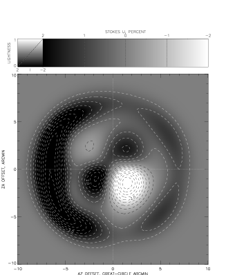
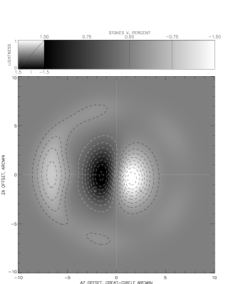
Figure 4.: Stokes $(I,Q,U,V)$ grey-scale/contour images of Arecibo’s main beam and first sidelobe near zenith angle $20\hbox{${}^{\circ}$}$. For $I$, solid (white) contours are $(0.1,0.2,\dots)$ of the peak; dashed (black) contours are $(0.01,0.02,\dots)$. For the others, black contours are for areas with negative $(Q,U,V)$ with the grey scale tending towards white; white contours are positive $(Q,U,V)$ with the greyscale tending towards black. Contours are in percent of Stokes $I$ at beam center and spaced by $0.4\%$ for $(Q,U)$ and $0.2\%$ for $V$; the $0\%$ contours are omitted. $U$ is aligned with the azimuth arm.

7.2. Main beam circular polarization

With circular polarization and a paraboloid having the feed aligned perfectly at the focal point, everything is circularly symmetric so there can be no beam structure in Stokes $V$. In practice, however, such perfection can never be achieved. If the feed points slightly away from the vertex of the paraboloid, say in the $X$ direction, then the two circularly polarized beams point in slightly different directions along the $Y$ direction. When the two circulars are subtracted to produce Stokes $V$, there is a two-lobed structure in the Stokes $V$ beam response. We call this beam squint; see Figure 4.

Arecibo and the GBT both employ an asymmetrically fed design in which the feed is both located off-axis and doesn’t point towards the center of symmetry. Thus, both have intrinsic beam squint built into their designs. One can minimize the polarization structure by appropriate design of the subreflector geometry. This optimization was done for both telescopes and, at least at Arecibo, the predicted main beam Stokes $V$ performance is close to what’s measured; the difference in direction $\sim 2$ arcsec.

7.3. Sidelobe polarization

Figure 4 shows the effects of beam squash and squint. They also show that the first sidelobe is highly polarized. As one moves away from beam center to encounter higher order sidelobes, the effects of distortion increase and the sidelobe polarizations increase. These effects are not well studied or understood.

Arecibo has a large central blockage produced by the suspended “triangle” structure from which the moving feed hangs. This produces large sidelobes (Heiles et al 2000b, 2001b), and these have high polarization. The GBT, with its unblocked aperture, has exceedingly low sidelobes, so effects arising from sidelobe polarization are minimized.

7.4. The effect on astronomical polarization measurements

Suppose one is observing a large-scale feature where the brightness temperature $T_{B}$ varies with position. One can express this variation by a two-dimensional Taylor expansion. Beam squint, by its nature, responds to the first derivative and only slightly to the second; beam squash responds primarily to the second.

The polarized beam structure produces fake results in the polarized Stokes parameters $(Q,U,V)$ that arise from spatial gradients in the total intensity Stokes parameter $I$. The effects are exacerbated by the polarized sidelobes, which are further from beam center.

Heiles et al (2000b, 2001b) calculated these effects for the Arecibo beam at 1.4 GHz, including both the main beam and first sidelobe but no additional sidelobes. Consider a total intensity gradient of 1 K arcmin^-1 and second derivative 1 K arcmin^-2, values which are not necessarily realistic but are convenient for practical use. For these particular values the the fake contributions from the first and second derivatives are comparable. They yield fake results for Stokes ${Q,U}\sim 0.3$ K. For Stokes $V$ the contributions are about ten times smaller, $\sim 0.03$ K.

The fractional polarization of extended emission tends to be small, so spatial gradients in $I$ can be very serious. Consider, for example, measuring Zeeman splitting of the 21-cm line in emission, which involves measuring Stokes $V$ of the 21-cm line. If the central velocity of the 21-cm line has a spatial gradient ${dv\over d\theta}=1$ km s^-1 deg^-1—a not-uncommon value as measured with a 36 arcmin beam (Heiles 1996)—we get $B_{fake}\sim 1.1$ $\mu$G. Gradients might be larger when measured with smaller $HPBW$. Typical values of $B$ are in the $\mu$G range, so this effect can be—but is perhaps not always—serious!

In principle, these effects can be corrected for. Correcting for them at Arecibo is a complicated business because of the $P\!A$ variation with azimuth and zenith angle. It is also an uncertain business, especially for $(Q,U)$ and somewhat less so for $V$, because these variations are unpredictable and must be determined empirically. Presumably, corrections at the GBT will be much more straightforward.

8. Summary

After a brief introduction to the astrophysical significance of polarization measurement, §2 began by introducing the Jones vector, which describes the polarization state of a sine wave. §3 went on to define the Stokes parameters and the Stokes vector, which are required to completely describe the polarization state of natural radiation, which is always at least partly randomly polarized. §3 also used the Stokes parameters to define the conventionally used quantities, fractional polarization and position angle, and cautioned against their use in arithmetic operations.

§4 related the Jones vector to the Stokes vector; this relationship tells exactly how radio astronomers measure all four Stokes parameters simultaneously. However, the receiving system modifies the incoming polarization with instrumental effects, which must be measured and corrected for; §5 described the quantitative aspects of this correction using Jones and Mueller matrices. It detailed the specific cases of the amplifier chain and the mechanical rotation of the telescope on the sky as instructive and most important examples. The Mueller matrix for the amplifier chain leads naturally to a discussion of the advantages of cross correlation for measuring small effects. It also shows how one must not use this falsely, as is often done using a post-amplifier hybrid.

Finally, §7 we described the major polarization effects in the main beam, namely beam squint and beam squash, and illustrated these effects using Arecibo as an example. Arecibo has a prominent first sidelobe, and §7 also discussed its rather severe polarization properties. It concluded by discussing of the effects of this beam structure, interacting with spatial derivatives in Stokes $I$, on contaminating measurements of polarized Stokes parameters.

Acknowledgments.

This work was supported in part by NSF grants 95-30590 and AST-0097417.

References

Hanaker, J.P., Bregman, J.D., & Sault, R.J. 1996, A&AS, 117, 137.

Heiles, C. 1996, ApJ, 466, 224.

Heiles, C. 1999, Arecibo Technical and Operations Memo 99-02.

Heiles, C. and Fisher, R. 1999, NRAO Electronics Division Internal Report 309.

Heiles, C., et al 2000a, Arecibo Technical and Operations Memo 2000-05.

Heiles, C., et al 2000b, Arecibo Technical and Operations Memo 2000-04.

Heiles, C. 2001, PASP, submitted.

Heiles, C., et al 2001a, PASP, submitted.

Heiles, C., et al 2001b, PASP, submitted.

Tinbergen, J. 1996, Astronomical Polarimetry, Cambridge Univ Press.

Troland, T.H. & Heiles, C. 1982, ApJ, 252, 179.