Chandra observations of the galaxy cluster Abell 1835

Abstract

We present the analysis of 30 ksec of Chandra observations of the galaxy cluster Abell 1835. Overall, the X-ray image shows a relaxed morphology, although we detect substructure in in the inner 30 kpc radius. Spectral analysis shows a steep drop in the X-ray gas temperature from $\sim$12 keV in the outer regions of the cluster to $\sim$4 keV in the core. The Chandra data provide tight constraints on the gravitational potential of the cluster which can be parameterized by a Navarro, Frenk & White (1997) model. The X-ray data allow us to measure the X-ray gas mass fraction as a function of radius, leading to a determination of the cosmic matter density of $\Omega_{\rm m}=0.40\pm 0.09\,h_{50}^{-0.5}$. The projected mass within a radius of $\sim$150 kpc implied by the presence of gravitationally lensed arcs in the cluster is in good agreement with the mass models preferred by the Chandra data. We find a radiative cooling time of the X-ray gas in the centre of Abell 1835 of about $3{\times}10^{8}$ yr. Cooling flow model fits to the Chandra spectrum and a deprojection analysis of the Chandra image both indicate the presence of a young cooling flow ($\sim 6{\times}10^{8}$ yr) with an integrated mass deposition rate of $230^{+80}_{-50}\,M_{\odot}$ yr^-1 within a radius of 30 kpc. We discuss the implications of our results in the light of recent RGS observations of Abell 1835 with XMM-Newton.

1 Introduction

Since its launch in 1999 July, the Chandra X-ray observatory (Weisskopf et al., 2000) has observed a large number of galaxy clusters, many of which are amongst the most massive objects of their kind. In particular, high resolution, spatially-resolved spectroscopy with the Advanced CCD Imaging Spectrometer (ACIS) on Chandra is leading to significant advances in the way we understand these systems.

As illustrated in a recent paper by Allen et al. (2001a), Chandra observations enable us to constrain the properties of galaxy clusters with unprecedented accuracy. Chandra data permit direct measurements of the X-ray gas density, temperature and total mass profiles at a resolution of $\sim 20$ h${}^{-1}_{50}$ kpc for the most massive clusters observed at redshifts $z\sim 0.2$, paving the way for detailed cosmological studies.

In this paper we present Chandra observations of the galaxy cluster Abell 1835 at a redshift $z=0.2523$. This cluster is the most luminous system ($L_{\rm X}=2.7\times\,10^{45}\,$ergs s^-1 in the 0.1-2.4 keV ROSAT band) in the ROSAT Brightest Cluster Sample (Ebeling et al., 1998) and has previously been inferred to contain a strong cooling flow (with a nominal mass deposition rate of $\sim 1000$ $\hbox{$\rm\thinspace M_{\odot}$}{\rm\thinspace yr}^{-1}\,$; e.g., Allen et al. 1996). The central dominant galaxy exhibits powerful optical emission lines and a strong UV/blue continuum associated with large amounts of ongoing star formation (Allen, 1995; Crawford et al., 1999). The observed Balmer emission line ratio also indicates significant intrinsic reddening (Allen, 1995, $E(B$-$V)=0.49^{+0.17}_{-0.15}$). This is consistent with the detection of 850 $\mu$m emission from the cD galaxy by Edge et al. (1999), which those authors attribute to emission from warm dust heated by the young, hot stars.

The great concentration of mass in the cluster is also revealed by several features in optical images that can be identified as gravitationally lensed background objects. In particular, a large arc was discovered by Edge et al. (in preparation) to the south-east of the cD galaxy. Allen et al. (1996) used this arc to put constraints on the cluster mass inside the radius of the arc. We will discuss several further possibly lensed objects in this study.

The structure of this paper is as follows: Sect. 2 describes the Chandra observations and Sect. 3 the basic imaging results. Sect. 4 discusses the spatially-resolved spectroscopy of the cluster using the Chandra data. Sect. 5 presents a detailed mass analysis using the independent X-ray and lensing data.In Sect. 6 we examine the properties of the central cooling flow and compare our results with those from recent observations made with the XMM-Newton X-ray observatory. We present our conclusions in Sect. 7. All quantities are given throughout using a cosmology with H${}_{0}=50$ km s^-1 Mpc^-1 and q${}_{0}=\frac{1}{2}$. Unless otherwise noted all error bars are 1 $\sigma$ (68.3%) confidence intervals.

2 Observations

Chandra observed Abell 1835 on 12 December 1999 for a total of 19.6 ksec. The target was centred in the middle of node 1 of the back-illuminated ACIS chip S3 (ACIS-S3), near the nominal aim point of this detector. The detector temperature during the observation was -110^° C. A further 10.7 ksec Chandra observation of Abell 1835 was obtained on 29 April 2000 at a detector temperature of -120^° C. In this second exposure, the cluster was centred close to the node boundary in the geometrical centre of the ACIS-S3 chip, in the middle of a group of five dead columns. This has prevented us from using this second data set for the spectral analysis presented in this paper. We have, however, used both data sets to produce the images in Figs. 1 and 4.

3 Imaging

In Fig. 1 a contour plot of the 30 ksec Chandra exposure of the inner region of the galaxy cluster in the 0.3-7.0 keV energy band is shown with a side length of 3.3 arcminutes (1 Mpc at the distance of the galaxy cluster). About 80,000 photons are collected in this image. For comparison, an archival 20 min B-band exposure taken on 27 February 1998 with the Canada France Hawaii Telescope (CFHT) of the central 1.5’$\times\,$1.5’ is shown in Fig. 2. In the optical image, the large arc (object A) discovered by Edge et al. (in preparation) can be seen to the south-east of the central cluster galaxy. This arc is thought to be a gravitationally lensed image of a galaxy far behind Abell 1835. The presence of this arc, notwithstanding the large X-ray emission, suggests that Abell 1835 is a very massive galaxy cluster. Allen et al. (1996) estimated the projected mass inside the radius of the arc to be between 1.4$\times 10^{14}$ M_⊙ and 2$\times 10^{14}$ M_⊙, if the arc has a redshift greater than 0.7 and is situated on a critical line of the gravitational potential of the cluster. In Fig. 2 a smaller arc can be seen to the south-west (object B) of the central cluster galaxy. The arrow to the north-west of the cD galaxy points to a radial feature which we discuss in Sect. 5.2.

Except for an apparent point source $\sim 1.5$ arcmin to the east (this is discussed in Fabian et al. 2000a and Crawford et al. 2000), the Chandra image is dominated by emission from the hot intracluster gas of the galaxy cluster. Overall, the cluster has a regular, relaxed morphology. The isophotes outside the core are elliptical with an axis ratio of minor and major axis $\sim\,0.85$. In Fig. 3, the average counts per sec per arcsec² as a function of radius are shown as counted in annuli around the galaxy cluster centre in the 0.3-7.0 keV band. The profile shows the steep surface brightness profile typical of cooling flow clusters (e.g., Fabian, 1994). Note, however, that Chandra detects a flattening of the profile within $r\sim 30\,$kpc.

Figure 1: X-ray contours of the central 3.3$\times$3.3 arcmin (1x1 Mpc) of Abell 1835 in the 0.3-7.0 keV band. The contours were drawn at 1, 2, 4, 8, 16, 32, 64, 91 and 108 counts per 1x1 arcsec pixel. The coordinates are J2000.

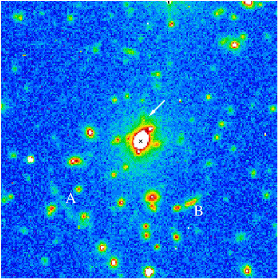
Figure 2: Optical B-band image of the inner 1.5’$\times$1.5’ (0.45$\times$0.45 Mpc) of Abell 1835. North is up and east is to the left. The cross marks the galaxy core. The greyscale has been wrapped once for clarity.

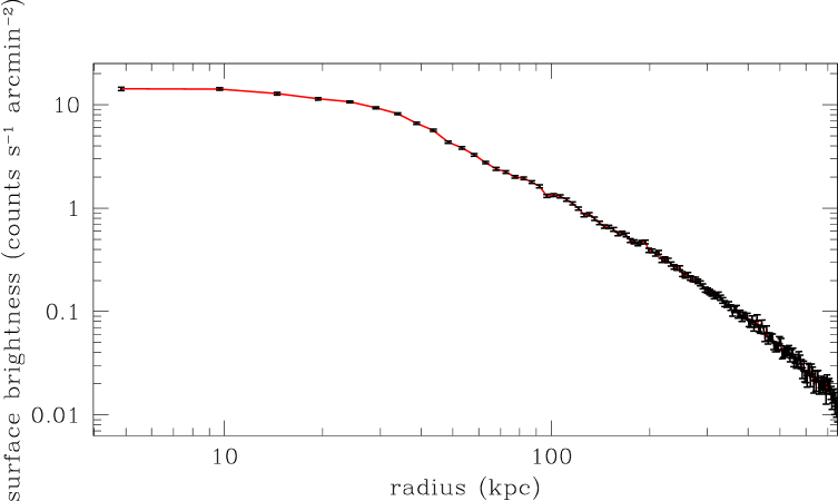
Figure 3: Surface brightness profile of Abell 1835 as a function of projected separation from the cluster centre. The count rates have been azimuthally averaged in annuli of width of 1 arcsec (4.9 kpc). The data points are positioned on the abscissa at the average of the inner and outer radius of the annuli. The data points are shown with Poisson error bars.

In Fig. 4 the central 30”$\times$30” (150 kpc side length) of Fig. 1 are shown. The image was smoothed with a Gaussian kernel with a full-width at half-maximum of 1.6 pixels (0.8 arcsec). In the inner 20 arcsec (100 kpc) of the cluster Chandra resolves substructure in the X-ray emission. There are a couple of main features visible: a well-defined peak just east of the geometrical centre (denoted by the black ring; J2000.0 coordinates given by Chandra: RA 14:01:02.07, DEC +2:52:43.2) of the cluster, a more inhomogeneous structure to the south-west of the geometrical centre, between these two regions an elongated strip with a reduced count rate, and a small emission front to the south-east of the cluster core (between the arrows in Fig. 4). The brightness gradient towards the north-west is steeper than towards the south-east. These features may be the sign of a merging subclump. The number of counts per half-arcsecond pixel in the brightest regions in the combined 30 ksec of our data is between 30 and 40. This means that the detailed structures need to be analysed with care because the Poisson error is still of the order of 20%. The main features, however, are robustly detected and indicate the presence of variations of the X-ray emission or absorption in the core of Abell 1835 on scales of several kiloparsecs. Comparison with the optical image (Fig. 2) shows that the emission inhomogeneities are situated inside the central cluster galaxy.

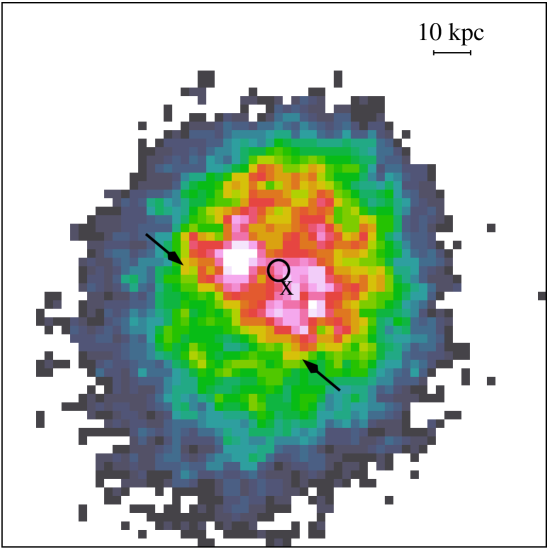
Figure 4: X-ray image of the central 30”$\times$30” (150 kpc$\times$150 kpc) of Abell 1835 in the 0.3-7.0 keV band. North is up and east is to the left. The image was smoothed with a Gaussian with a full-width at half-maximum of 0.8 arcsec. The pixels are 0.5x0.5 arcsec. Only pixels with at least 6 counts are plotted. The circle marks the geometrical centre of the cluster mentioned in the text. The cross marks the absolute position of the galaxy core (see Fig. 2) determined by Allen et al. (1996) when plotted in the coordinates given by Chandra. The uncertainties associated with the galaxy position and the Chandra astrometry are $\sim\,1$ arcsec. The two arrows point at the small emission front extending between them. The greyscale has been wrapped once for clarity.

4 Spatially resolved spectral analysis

4.1 Data extraction

We extract spectra from selected regions of the longer 19.6 ksec exposure Chandra data set using the CIAO software package distributed by the Chandra X-ray Observatory Centre (CXC, web site: cxc.harvard.edu).

We only work with photons detected in the ACIS-S3 chip, which is also known as ACIS chip 7. This is a back-illuminated chip and does not suffer from the degradation of energy resolution that affects the front-illuminated ACIS chips on the Chandra observatory. All significant point sources were masked out and excluded from the analysis.

Response matrix files (RMF) and ancillary response files (ARF) were produced using a PERL script generously provided to us by Roderick Johnstone. This script combines individual RMFs and ARFs for each 32x32 pixel region on the ACIS-S3 chip (generated using the mkrmf tool in the CIAO software suite available from the CXC website) in a photon number-weighted manner.

Using the task grppha from the FTOOLS software package provided by the NASA High Energy Astrophysics Science Archive Research Center (HEASARC, FTOOLS web site: heasarc.gsfc.nasa.gov/lheasoft/ftools/) we have grouped the extracted spectra so that we have at least 20 counts in a bin corresponding to a certain range of energy channels. We can then use Poisson error bars to account for the uncertainty in the number of photons per bin.

We have have generated background spectra using Maxim Markevitch’s method and program that is available from the CXC web site. We extract the background data from the same regions on the chip as the spectra extracted from the Abell 1835 data set. We also scanned the light curve of the Abell 1835 data for flares or background activity using the tool lc_clean provided by Markevitch. The light curve is stable throughout the 19.6 ksec exposure.

4.2 Colour profile analysis

In order to illustrate the spectral energy distributions from different regions in Abell 1835 we have firstly constructed an X-ray colour profile. Two separate images were created in the energy bands $0.5-1.3$ and $1.3-7.0$ keV ($0.6-1.6$ and $1.6-8.8$ keV in the rest frame of the source) with a 1.97 arcsec (4 raw detector pixels) pixel scale. These soft and hard X-ray images were background subtracted and flat fielded (using the exposure map tools available on the CXC web site and taking full account of the spectral energy distributions of the detected photons). Azimuthally-averaged surface-brightness profiles for the cluster were then constructed in each energy band, centred on the geometrical centre of the X-ray emission. The colour profile formed from the ratio of the surface brightness profiles in the soft and hard bands is shown in Fig. 5.

From examination of Fig. 5 we see that at large radii the observed X-ray colour ratio is approximately constant, with a mean value of $1.05\pm 0.03$ ($1\sigma$ error determined from a fit to the data between radii of $200-400$ kpc). Within a radius of $\sim$30 arcsec (150 kpc), however, the colour ratio rises, indicating the presence of cooler gas.

Figure 5: X-ray colour profile of the central 1.7 arcmin (500 kpc) of Abell 1835. In this figure the ratio of the azimuthally averaged counts in the $0.5-1.3$ and $1.3-7.0$ keV bands ($0.6-1.6$ and $1.6-8.8$ keV in the rest frame of the source) is plotted as a function of the radius of the annuli.

4.3 Single-temperature model

We investigate now the temperature profile that causes the colour profile shown in Fig. 5. To do this we have extracted spectra from annuli around the geometrical centre (marked by the black circle in Fig. 4) of the X-ray emission with photon energies in the 0.5-7.0 keV band. We use a slightly smaller energy band for the spectral analysis than we used for the images in order to get robust answers at soft energies. The annuli have widths of 5, 10, 25, 50 and 100 arcsec (25, 50, 125, 250 and 500 kpc, respectively) and provide sufficient counts (see Tab. 1) to study the spectral properties of the X-ray gas.

We use the software package XSPEC (Arnaud, 1996) to model the spectra with the MEKAL plasma emission model (Kaastra & Mewe, 1993; Liedahl et al., 1995) multiplied by the PHABS (Balucinska-Church & McCammon, 1992) photoelectric absorption model

$${\rm MODEL}_{1}={\rm PHABS}\,(N_{\rm H})\,\times\,{\rm MEKAL}\,(T;Z;K).$$ (1)

The free model parameters are indicated in brackets: the absorbing equivalent hydrogen column density $N_{\rm H}$, the gas temperature $T$, the metallicity $Z$ (in units of solar abundance), and a normalization factor K.

An account of the relevant parameters and the model fits is given in Table 1. All our fits are statistically acceptable, with reduced $\chi^{2}$ values of around or slightly above unity. Since the absorbing column density and the metallicity are not well constrained in the outer annuli, we have also carried out a second analysis in which we grouped the data into three larger regions. This procedure eliminates free parameters and thus yields more robust estimates. The results are shown in Table 2.

It can be seen from Table 2 that the spectra from annuli with inner radii larger than 30 arcsec (150 kpc) are consistent with Galactic absorption (Dickey & Lockman, 1990). We have thus repeated the isothermal model fits according to eq. (1) for these annuli with fixed Galactic absorption. The corresponding best-fit models are also given in Table 1. For the outermost annuli, this leads to a smaller predicted temperature with smaller uncertainties.

In Fig. 6 the results from the model fitting for the ambient gas temperature $T$ are plotted. For annuli with inner radii $\geq$30 arcsec (150 kpc), we have fixed the absorbing column density to the Galactic value. The best-fit temperatures reveal a strong drop from $kT\sim\,12$ keV in the outer regions of the cluster down to 4 keV in the centre of the cluster. We note that the photons in the annuli have been emitted in a hollow cylinder with a cross-section given by the annulus. The measured temperatures are fits to the spectrum from this whole region and thus have to be regarded as average (emission weighted) temperatures.

Table 1: Isothermal model fits. The model described in eq. (1) with the free parameters equivalent hydrogen column density $N_{\rm H}$, temperature T and metallicity $Z$ was fitted to spectra extracted from annuli around the geometrical centre of Abell 1835 with inner radii $r_{1}$ and outer radii $r_{2}$. For annuli with $r_{1}\geq 250\,$kpc (50 arcsec) we have modelled the X-ray spectra from the annuli both with free equivalent hydrogen column density $N_{\rm H}$ (top block of models), and with fixed Galactic absorption (Dickey & Lockman, 1990, bottom block of models). Since neither the metallicity nor the absorbing column density can be smaller than zero, the lower limit has always been fixed accordingly for these parameters. In columns 6 and 7 we list the total number of counts and the expected number of background counts in the 0.5-7.0 keV band. In the last three columns the $\chi^{2}$ values, the number of degrees of freedom (DOF) and the reduced $\bar{\chi}^{2}=\chi^{2}$/DOF are given.

$r_{1}$ (kpc)	$r_{2}$ (kpc)	kT (keV)	$Z$ (solar)	$N_{\rm H}$ (1020 cm-2)	counts	exp. background	$\chi^{2}$	DOF	$\bar{\chi}^{2}$
0	25	4.0${}^{+0.3}_{-0.3}$	0.24${}^{+0.07}_{-0.07}$	3.93${}^{+0.82}_{-0.82}$	4791	2.4	148.1	122	1.21
25	50	4.7${}^{+0.2}_{-0.2}$	0.31${}^{+0.05}_{-0.06}$	3.97${}^{+0.66}_{-0.64}$	8300	8.5	218.1	161	1.35
50	100	7.5${}^{+0.5}_{-0.4}$	0.28${}^{+0.06}_{-0.07}$	3.27${}^{+0.58}_{-0.55}$	10776	27.0	233.8	193	1.21
100	150	8.5${}^{+0.7}_{-0.7}$	0.39${}^{+0.10}_{-0.10}$	2.29${}^{+0.66}_{-0.65}$	7680	51.2	186.3	172	1.08
150	250	9.1${}^{+0.8}_{-0.7}$	0.35${}^{+0.08}_{-0.09}$	3.00${}^{+0.60}_{-0.58}$	10527	138.7	203.6	195	1.04
250	375	8.0${}^{+0.8}_{-0.6}$	0.30${}^{+0.09}_{-0.10}$	4.75${}^{+0.75}_{-0.74}$	7838	262.6	177.0	164	1.08
375	500	12.5${}^{+3.7}_{-1.9}$	0.49${}^{+0.27}_{-0.24}$	1.86${}^{+0.96}_{-1.14}$	5466	378.0	135.6	124	1.09
500	750	16.9${}^{+5.1}_{-3.2}$	0.20${}^{+0.45}_{-0.20}$	0.07${}^{+2.11}_{-0.07}$	7003	1123.4	159.2	169	0.94
750	1250	26.0${}^{+2.8}_{-11.2}$	0.00${}^{+0.52}_{-0.00}$	0.00${}^{+0.29}_{-0.00}$	8322	3075.7	198.0	199	1.00
150	250	9.7${}^{+0.6}_{-0.6}$	0.35${}^{+0.09}_{-0.09}$	2.30	10527	138.7	205.0	196	1.05
250	375	10.0${}^{+0.8}_{-0.8}$	0.32${}^{+0.12}_{-0.12}$	2.30	7838	262.6	188.1	165	1.14
375	500	11.9${}^{+1.9}_{-1.4}$	0.48${}^{+0.26}_{-0.23}$	2.30	5466	378.0	135.8	125	1.09
500	750	13.1${}^{+2.1}_{-1.6}$	0.22${}^{+0.21}_{-0.12}$	2.30	7003	1123.4	162.3	170	0.95
750	1250	12.5${}^{+3.5}_{-2.4}$	0.23${}^{+0.36}_{-0.23}$	2.30	8322	3075.7	207.6	200	1.04

Table 2: Model parameters for isothermal models using combined sets of data. The spectra from annuli around the cluster centre as used in Table 1 have been fitted simultaneously using the same absorbing column density and metallicity for all annuli in the range $r_{1}\rightarrow\,r_{2}$ and by allowing for different temperatures in each of the annuli of Table 1. The last three columns, as in Table 1, describe the number of degrees of freedom and the quality of the fits.

	$r_{1}$ (kpc)	$r_{2}$ (kpc)	$Z$ (solar)	$N_{\rm H}$	$\chi^{2}$	DOF	$\bar{\chi}^{2}$
						(1020 cm-2)	(1020 cm-2)
	0	50	0.29${}^{+0.05}_{-0.04}$	3.94${}^{+0.51}_{-0.51}$	367.0	285	1.29
	50	150	0.31${}^{+0.06}_{-0.05}$	2.88${}^{+0.44}_{-0.43}$	422.0	367	1.15
	150	1250	0.31${}^{+0.07}_{-0.06}$	2.55${}^{+0.38}_{-0.36}$	898.9	857	1.05

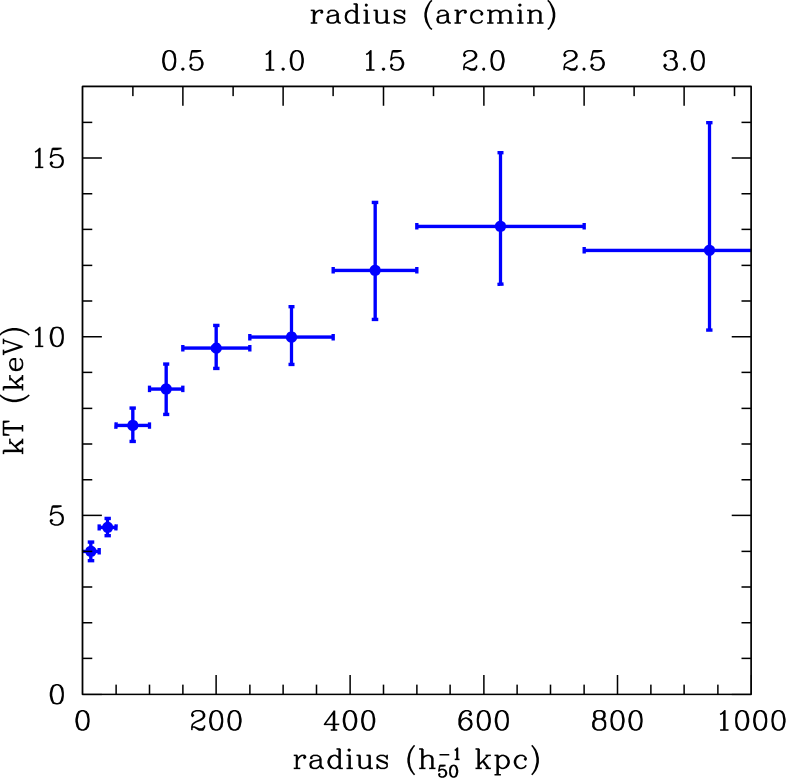
Figure 6: Temperature kT as a function of radius $r$ from the cluster centre out to 3.3 arcmin (1 Mpc). For data points at radii $\geq 30$ arcsec (150 kpc), we have plotted the temperatures derived using models with the absorption fixed at the Galactic value.

We have plotted the metallicity and absorption results of Table 2 in Fig. 7. The metallicity appears approximately constant with radius. We find tentative evidence that the isothermal model requires excess absorption above the Galactic value in the inner 100 kpc.

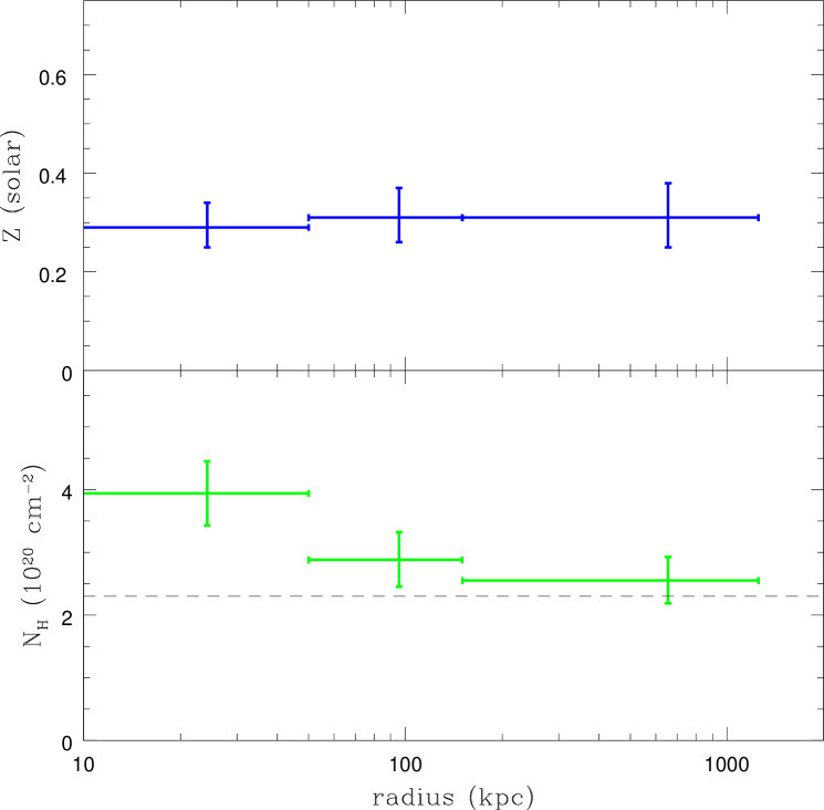
Figure 7: As in Fig. 6, but for metallicity $Z$ (in units of solar abundance) and photoelectric absorption column density $N_{\rm H}$ as determined from the combined fits in Table 2 to X-ray spectra extracted from annuli at several radii. In the lower panel, the Galactic absorption value from H I studies is indicated by the dashed line.

As an aside, we mention that if we apply model (1) to the spectrum extracted from a circle with a radius of 30 arcsec (150 kpc) and leave the Ni abundance as an additional free parameter, we find a Ni abundance of $2.3\pm 0.8$ times solar in this region. This relatively high Ni abundance is relevant for models of Type Ia supernovae and their enrichment of the intergalactic medium (e.g., Dupke & White, 2000).

4.4 Spectral deprojection analysis

The results discussed in the previous section are based on the analysis of projected spectra. In order to determine the effects of projection, we have also carried out a deprojection analysis of the Chandra spectra using the method described by Allen et al. (2001a). This method decomposes the observed annular spectra (Table 1) into the contributions from the X-ray gas emission from nine spherical shells.

The data for all nine annular spectra were fitted simultaneously in order to correctly determine the parameter values and confidence limits. The spectral model used therefore has $2\,n+1$ free parameters (where $n=9$ is the number of annuli), corresponding to the temperature and emission measure in each spherical shell and the overall emission-weighted metallicity (the metallicity is linked to take the same value at all radii, yielding a metallicity $Z=0.32^{+0.03}_{-0.04}$). The absorbing column density was fixed at the Galactic value. The temperature profile determined with the spectral deprojection code is shown in Fig. 8.

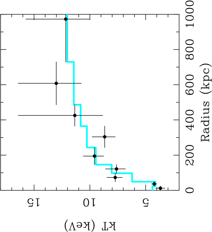
Figure 8: Deprojected temperature profile of Abell 1835. The solid line is the best-fit temperature profile determined in Sect. 5.1.

5 X-ray mass analysis

5.1 The mass model

The observed X-ray surface brightness profile (Fig. 3) and deprojected X-ray gas temperature profile (Fig. 8) may together be used to determine the X-ray gas mass and total mass profiles in the cluster. For this analysis, we have used an enhanced version of the deprojection code described by White, Jones and Forman (1997) and have followed a similar method to that described by Allen, Ettori & Fabian (2001a). Spherical symmetry and hydrostatic equilibrium are assumed.

A variety of simple parameterizations for the cluster mass distribution were examined, to establish which could provide an adequate description of the Chandra data. We find that the Chandra data can be modelled using a Navarro et al. (1997) (NFW) mass model

$$\rho(r)={{\rho_{\rm crit}\,\delta_{\rm c}}\over{({r/r_{\rm s}})\left(1+{r/r_{\rm s}}\right)^{2}}},$$ (2)

where $\rho(r)$ is the mass density, $\rho_{\rm crit}=3H(z)^{2}/8\pi G$ is the critical density for closure of the universe ($H(z)$ is the Hubble constant and G is the gravitational constant) and

$$\delta_{\rm c}=\frac{200}{3}\frac{c^{3}}{{{\rm ln}(1+c)-{c/(1+c)}}},$$ (3)

where $c$ is the concentration parameter. The normalization of the mass profile may also be expressed in terms of an effective velocity dispersion, $\sigma=\sqrt{50}H(z)r_{\rm s}c$.

We step the mass model parameters $r_{\rm s}$ and $\sigma$ through a regular grid of values. (The scale radius $r_{\rm s}$ was stepped between 0.1 Mpc and 2.5 Mpc and the effective velocity dispersion $\sigma$ between 500 km s^-1 and 2500 km s^-1 on a grid of 81$\times$81 models.) Given the observed surface brightness profile and a particular parameterized mass model, the deprojection code is used to predict a temperature profile of the X-ray gas (we use the median model temperature profile determined from 100 Monte-Carlo simulations) which is then compared for each mass model with the observed, deprojected temperature profile (Fig. 8).

We have determined the goodness of fit of each simulated temperature profile by calculating the sum

$$\chi^{2}=\sum_{\,\rm all\,radial\,bins}\,\left(\frac{T_{\,\rm obs}-T_{\,\rm model}}{\sigma_{\,\rm obs}}\right)^{2},$$ (4)

where $T_{\,\rm obs}$ is the observed deprojected temperature profile shown in Fig. 8 and $T_{\,\rm model}$ is the model temperature profile, rebinned to the same spatial scale using an appropriate flux weighting.

Fig. 8 shows the X-ray gas temperature profile implied by the best-fitting NFW mass model ($\chi^{2}=11.9$ for $r_{\rm s}=0.64^{+0.21}_{-0.12}$ Mpc, $\sigma=1275^{+150}_{-100}\,$km s^-1 and $c=4.0^{+0.54}_{-0.64}$) overlaid on the deprojected temperature profile. The $\chi^{2}$ value is mostly due to the differences between model and data close to the cluster centre, and may at least in part be attributed to the asymmetric substructure seen in Fig. 4.

Fig. 9 shows a contour plot of the $\chi^{2}$ values calculated for the different NFW models in the parameter space. The minimum $\chi^{2}$ value is marked by a plus sign. Three contours have been drawn at differences of $\Delta\chi^{2}=$ 2.3, 6.17 and 11.8, corresponding to formal confidence intervals of 68.3% (1 $\sigma$), 95.4% (2 $\sigma$) and 99.73% (3 $\sigma$) for the two parameters (e.g., Press et al., 1992, page 661). Fig. 10 shows the $1\,\sigma$ range of enclosed masses for models around the best-fit model both for the total mass inside a sphere of radius $r$ and for the total projected mass inside a radius $r$ (using the mass formula by Bartelmann 1996). The mass inside a sphere with the virial radius $r_{200}=c\times{r_{\rm s}}$ for the best-fit model is $M_{200}=2.7^{+0.5}_{-0.7}\times 10^{15}\,M_{\odot}\,$yr^-1.

We note that it is also possible to carry out this analysis with a nonsingular isothermal mass density profile

$$\rho(r)=\frac{\sigma_{\rm iso}^{2}}{2\,\pi\,{\rm G}}\,\frac{1}{r^{2}+r_{\rm c}^{2}},$$ (5)

where $\sigma_{\rm iso}$ is the velocity dispersion and $r_{\rm c}$ is the core radius. This yields parameters $r_{\rm c}=65.0^{+5.0}_{-10.0}\,$kpc and $\sigma_{\rm iso}=1280\pm 60\,$km s^-1. The fit is slightly better, $\chi^{2}=6.8$, but the conclusions we can draw from both profiles regarding the total mass and X-ray gas profiles are very similar.

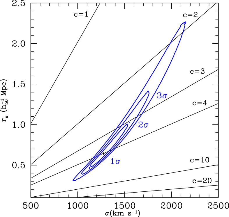
Figure 9: Contour plot of the 68.3% ($1\sigma$), 95.4% ($2\sigma$) and 99.73% ($3\sigma$) formal confidence contours on the NFW scale radius $r_{\rm s}$ and effective velocity dispersion $\sigma$. For this, a grid of $81\times 81$ mass models was graded using the $\chi^{2}$ statistic by comparing the predicted temperature profile with the deprojected Chandra temperature profile. Also shown for reference are the isocontours of the NFW concentration parameter $c$. The minimum $\chi^{2}$ model with $\chi^{2}=11.9$ is marked by a plus sign.

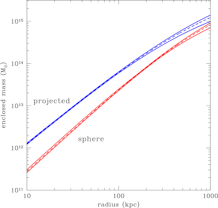
Figure 10: $1\,\sigma$ range and average value (dashed line) of the enclosed mass inside a sphere of radius $r$ and the total projected mass inside a radius $r$.

5.2 Lensing predictions from the X-ray mass models

In Fig. 11 (left panel) an optical B-R colour image is shown of the central 1.5$\times$1.5 arcmin of Abell 1835. The image has been constructed from the 20 min B-band image shown in Fig. 2 and a 10 min R-band image from the same observing run that was also taken from the CFHT archive. In this greyscale image, blue objects appear black, and red objects appear white. The contrast has been stretched that very faint objects can be seen. The two vertical stripes are due to bleeding columns in the R-band image that fortunately did not affect the cD galaxy.

In the central part of Fig. 11 (left panel), it can be seen that only the cD galaxy appears blue. The two arcs to the south east and south west of the cD galaxy were already pointed out in Fig. 2. The larger arc to the south east was discovered by Edge et al. (in preparation). The other arc has not been discussed in the literature so far. No redshift has been determined for either object in the literature, but their optical appearance and colours indicate that they are gravitationally lensed images of background galaxies that are situated at some distance behind the galaxy cluster (e.g., Schneider, Ehlers & Falco, 1992).

In the R-band image (not shown) we find a further pair of very thin and elongated features parallel to, but 9 arcsec south of the south east arc (termed C1 and C2 in the following). This pair of arcs is too faint to be seen in Fig. 11 (left panel). The total length of the pair is comparable to arc A, but is only barely visible in the B-band image. If we assume that the very faint B-band brightness of the pair is due to the redshifting of the Lyman break out of the B-band filter used (3800-4800 Å), we may deduce a redshift of $z\geq 4.0$ for this object pair (e.g., Madau et al., 1996).

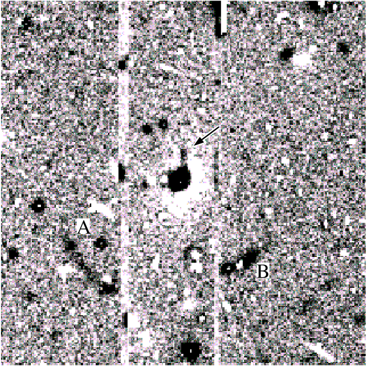
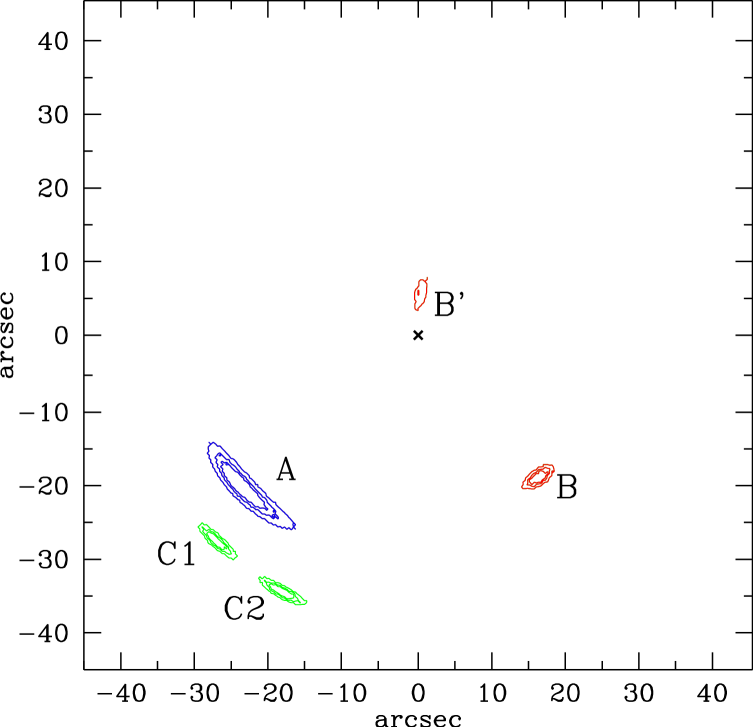
Figure 11: (left panel) B-R colour difference image of the central 1.5$\times$1.5 arcmin of Abell 1835 from archival CFHT data. North is up and East is to the left. The greyscale-contrast has been stretched to show blue objects in black and red objects in white. The two vertical features to the left and right of the central cD galaxy are due to bleeding CCD columns in the R-band image that were caused by bright stars to the north of the field. We have replaced the pixel values in these columns by the median background value. Features of particular interest in this image are the very blue central part of the cD galaxy and the two arcs to the south east (A) and south west (B) of the galaxy. We also note that to the north of the cD galaxy a straight blue feature is seen (arrow). (right panel) Contour plot of gravitationally lensed images by an elliptical NFW profile with a concentration parameter $c=3.3$, scale radius $r_{\rm s}=900\,$kpc, ellipticity $e=0.2$ and position angle of 330 degrees (measured counterclockwise from north). The cluster centre is marked by the cross. See the text for details on source positions, redshifts and sizes. The images have been labelled with upper case letters. B’ is the predicted counter arc of arc B.

The separations of the centres of arcs A and B from the centre of the cD galaxy are $\theta_{\rm A}\sim 31.1$ arcsec and $\theta_{\rm B}\sim 25.0$ arcsec. In a circularly symmetric gravitational lens, arcs appear close to the Einstein radius $\theta_{\rm E}$

$$\theta_{\rm E}=\sqrt{\frac{D_{{\rm clus-arc}}}{D_{\rm clus}\,D_{\rm arc}}\frac{4\,{\rm G}\,M}{c^{2}}},$$ (6)

where $M$ is the enclosed mass (e.g., Schneider et al., 1992). $D_{\rm clus}=1.02\,$Gpc, $D_{\rm arc}$ and $D_{\rm clus-arc}$ are the angular size distances of the cluster, the arc, and between cluster and arc. G is the gravitational constant and $c$ is the speed of light. For the case of Abell 1835, Allen et al. (1996) calculated the mass in a circular aperture inside arc A (their Fig. 13) and found a value between 1.4$\times 10^{14}$ M_⊙ and 2$\times 10^{14}$ M_⊙ for values of the redshift of the arc $0.6<z_{\rm arc}<3.0$. Similar values follow for arc B.

The NFW mass models in the region of best goodness of fit in Fig. 9 have only little variation of the total mass inside 31.1 arcsec (153 kpc): If we use the Bartelmann (1996) formulae for the total mass in a circular NFW profile, the $1\sigma$ formal confidence interval data ranges from $M_{\rm X}=1.06\times\,10^{14}\,M_{\odot}$ to $M_{\rm X}=1.27\times\,10^{14}\,M_{\odot}$ (Fig. 10). The values agree with the $1.26^{+0.32}_{-0.17}\times 10^{14}\,M_{\odot}$ determined using ROSAT data by Allen (1998). The values are lower, however, than the estimate from the lensing argument assuming circular symmetry.

From the X-ray image in Fig. 4 we can deduce that in the inner parts the X-ray isocontours are elliptical with an axis ratio of $f=0.85$ (Sect. 3). This suggests that also the mass distribution of Abell 1835 is not circularly symmetric. Numerical simulations by Bartelmann (1995) showed that the lensing mass estimate under the assumption of circular symmetry needs to be corrected towards lower values. As an average correction factor he quotes 1.6, but this may vary downwards to unity and upwards to $\sim$2 from case to case. For the lensing mass estimate the ellipticity thus could be an important factor. In order to go beyond the approximation of circular symmetry, we need to use an elliptical mass model.

The normalized surface mass density $\kappa=\Sigma/\Sigma_{\rm crit}$ of a spherical NFW mass distribution was derived by Bartelmann (1996). Using the ratio $x=r/r_{\rm s}$ of radius $r$ and scale radius $r_{\rm s}$ this is given by

$$\kappa(x)=2\,\kappa_{\rm s}\,\frac{f(x)}{x^{2}-1},$$ (7)

where

$$f(x)=\left\{\begin{array}[]{lc}1-\frac{2}{\sqrt{x^{2}-1}}\,{\rm arctan}\,\sqrt{\frac{x-1}{x+1}}&(x>1)\\ 1-\frac{2}{\sqrt{1-x^{2}}}\,{\rm arctanh}\,\sqrt{\frac{1-x}{1+x}}&(x<1)\\ 0&(x=1)\end{array}\right.$$ (8)

($\kappa\,(1)=\frac{2}{3}\,\kappa_{\rm s}$) and $\kappa_{\rm s}=\delta_{\rm c}\,\rho_{\rm crit}\,r_{\rm s}\,\Sigma^{-1}_{\rm crit}$. The critical surface mass density $\Sigma_{\rm crit}$ is given by

$$\Sigma_{\rm crit}=\frac{c^{2}}{4\,\pi\,{\rm G}}\,\frac{D_{\rm arc}}{D_{\rm clus}\,{D_{\rm clus-arc}}},$$ (9)

with constants as described after eq. (6). One can then generalize eq. (7) for a mass distribution with elliptical symmetry by making the transformation

$$x\rightarrow x_{\rm e}=\sqrt{\frac{x_{1}^{2}}{(1+\epsilon)^{2}}+\frac{x_{2}^{2}}{(1-\epsilon)^{2}}}$$ (10)

(Schramm, 1990, 1994; Kassiola & Kovner, 1993; Kormann, Schneider and Bartelmann, 1994) where $x_{1}$ and $x_{2}$ are cartesian coordinates and $\epsilon$ is the elliptical parameter. The elliptical parameter $\epsilon$ is related to the axis ratio $f$ via $f=\frac{1-\epsilon}{1+\epsilon}$. Using the summation method developed by Schramm (1994) we can then construct gravitational lens models for the elliptical NFW mass model within the viable range of parameters from Fig. 9. We use an axis ratio $f=0.8$ and a position angle of 330 degrees (measured counterclockwise from north) taken from the optical appearance of the cD galaxy. We do not use the axis ratio of the X-ray gas because the gas pressure causes the gas distribution to be more circular than the mass distribution (e.g., Buote & Canizares, 1996). We fix the centre of the mass model to the optical centre of the cD galaxy.

Without redshift information about the arc candidates, any parameterized lens modelling of the system is degenerate with respect to the mass normalization of the cluster. It is also necessary to make an assumption about whether to interpret the arcs as single images which have been elongated by the lens effect, or as fold-arcs consisting of two mirror images of the same object (e.g., Schneider et al., 1992). Since we do not detect counter images for arc A, it is likely that it is a single, elongated image of background galaxy. We also cannot detect a counter image for the pair C1/C2 in the CFHT R-frame, which could indicate that they are bright spots in a common, darker background galaxy that appears elongated by the lens effect. On the basis of the archival CFHT data, however, it is impossible to identify unambiguously which images belong together, or to rule out the existence of further counter images.

We have first studied the lens effect of an NFW model with $\sigma=1460\,$km s^-1 and $r_{\rm s}=0.9\,$Mpc, which is situated inside the $1\,\sigma$ confidence region in Fig. 9. With this mass distribution, arc A can be explained as a single elongated image of a background galaxy at $z_{\rm A}\sim 2.7$. The arc pair C1/C2 in this model are images of two objects at $z_{\rm C}\sim 5.0$ with a projected physical (unlensed) separation of $\sim 10\,$kpc. This redshift is consistent with our limit $z_{\rm C}\geq 4.0$ which was obtained from the fact that the pair is not visible in the CFHT B-frame. An arc at the position of arc B is predicted for several source redshifts, but the most interesting interpretation is a background object at $z_{\rm B}\sim 2.25$, because at this redshift the lens model predicts counter images in the form of a radial arc at the position of the straight blue feature to the north of the cD (Fig. 11, left panel; the existence of radial arcs in NFW profiles was shown by Bartelmann 1996).

The image configuration predicted by this model is shown in the right panel of Fig. 11. Circular Gaussian brightness profiles have been assumed for all sources with a full width at half maximum of 0.45 arcsec for source A and 0.25 arcsec for sources B, C1 and C2. The contours have been spaced at 10%, 30% and 50% of the central surface brightness. The assumed source positions on the sky with respect to the cluster centre in the form $(\Delta x$, $\Delta y)$ are: source A: ($-5.06$”, $-6.20$”), source B: ($0.50$”, $-2.44$”), source C1: ($-7.05$”, $-9.03$”), source C2: ($-5.78$”, $-10.22$”).

Secondly, since arc A appears roughly symmetric (Fig. 11, left panel), we have also investigated the possibility that it is a fold-arc. This interpretation may be supported by the similarity of arcs C1 and C2. We find, however, that none of the models inside the $1\,\sigma$ confidence region in Fig. 9 are massive enough to explain a fold-arc at the radius of arc A (31.1 arcsec or 153 kpc). In this case it would be necessary to scale the surface mass density $\kappa\rightarrow\kappa^{\prime}=q\times\kappa$ of all models in the formal $2\,\sigma$ contour by correction factors between $q=1.1$ and $q=1.4$. The redshift of arc A in such models would typically be $z_{\rm A}\sim 2.0$. (The redshift is constrained to be around $z_{\rm A}\sim 2.0$ because it is also necessary to explain arcs B and C1/C2. Arc B would have a redshift $z_{\rm B}\sim 0.9$. C1 and C2 would be interpreted as images of a source at $z_{\rm C}>4.2$. The radial feature to the north of the cD could again be interpreted in this model as a radial arc.)

We have also studied different axis ratios within the context of the fold-arc model: Lowering the axis ratio reduces the correction factor $q$ because the ellipticity causes the critical curve to extend further out. We thus find that elliptical $f\sim 0.6$ models within the $2\sigma$ confidence contour of Fig. 9 are able to explain the CFHT data. The axis ratio should be larger than $f=0.5$, however, because otherwise it is not possible to have an elongated arc at the position of arc B (without additional perturbations of the potential). By using nonsingular isothermal mass profiles (eq. (5)) the correction factor $q$ can also be reduced further.

Our analysis clearly favours the first, single-image, interpretation of arc A, as well as C1/C2, because the fold-arc model predicts counter-images for arcs A, C1/C2 that are not observed. The available strong lensing data are explained by a mass model entirely consistent with the Chandra temperature profile, indicating that there are no significant contributions from non-thermal sources of pressure (e.g., bulk motions, magnetic fields). The fold-arc models require special tuning of the mass distribution, although it may be possible to explain the additional mass with systematic uncertainties of our X-ray mass analysis due to the residual substructure seen in the X-ray emission, or by a merging subcluster or some other line-of-sight enhancement present in this region. Nevertheless, the predicted counter images would have to be found before this option can be considered further.

We have not attempted any more detailed lens modelling including sub-halos due to cluster member galaxies because the available data are of insufficient quality to unambiguously establish the arc properties and identify image pairs. A more rigorous analysis aiming to place precise constraints on the redshifts of the arcs and corresponding arc properties is a subject for future study and will best be done with the Hubble Space Telescope (Kneib, 2000; Smith et al., 2000). Moreover, spectroscopy will be required in order to ensure that the arc candidates are indeed galaxies at high redshift (e.g., Ebbels et al., 1998). A measurement of the redshift of arc B alone would provide a very strong test of the mass models discussed here.

5.3 The X-ray gas mass fraction

The X-ray gas-to-total-mass ratio as a function of radius, $f_{\rm gas}(r)$, determined from the Chandra data is shown in Fig. 12. For this figure, the gas mass fraction was calculated for all models contained in the $1\,\sigma$ confidence contour of Fig. 9. The dashed line corresponds to the best-fit model, the solid lines are the envelopes of all calculated profiles. The $f_{\rm gas}$ value rises rapidly with increasing radius within the central $\sim 50$ kpc and then flattens, remaining approximately constant out to the limits of the data at $r=1.0$ Mpc, where we measure $f_{\rm gas}=0.171^{+0.020}_{-0.022}h_{\rm 50}^{-1.5}$.

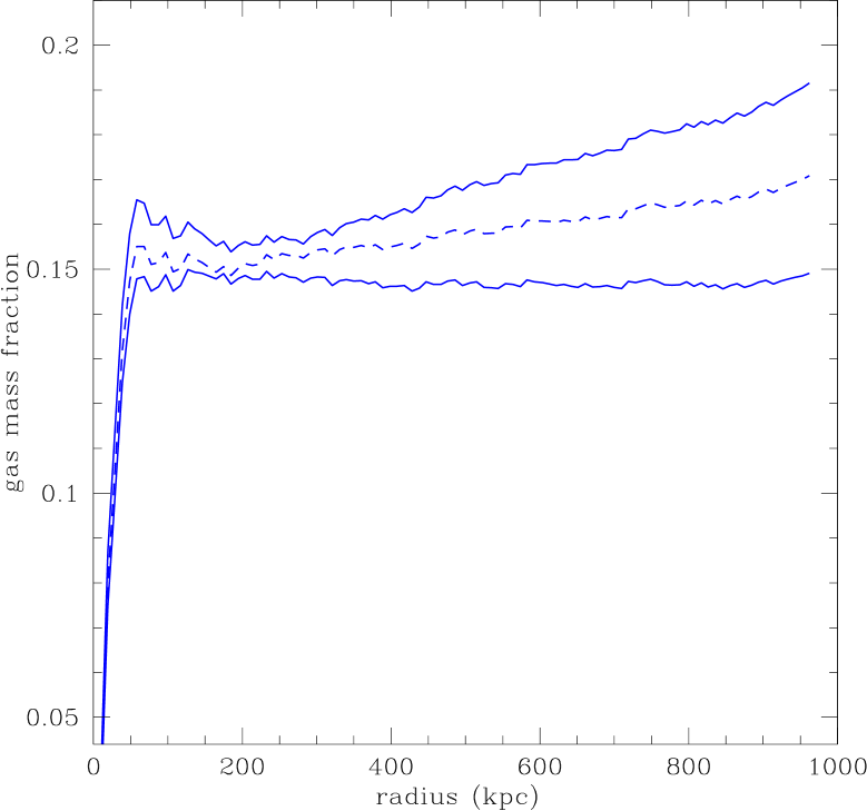
Figure 12: Upper and lower $1\,\sigma$ limits on the gas mass fraction fraction as a function of radius $r$. In addition, for reference the gas mass fraction has been plotted also for the best-fit model $r_{\rm s}=0.64$ Mpc, $\sigma=1275\,$km $s^{-1}$ (dashed line).

Following the usual arguments, which assume that the properties of clusters provide a fair sample of those of the Universe as a whole (e.g., White, Efstathiou & Frenk 1993; White & Fabian 1995; Evrard 1997; Ettori & Fabian 1999), we may use our result on the X-ray gas mass fraction in Abell 1835 to estimate the total matter density in the Universe, $\Omega_{\rm m}$. Assuming that the luminous baryonic mass in galaxies in Abell 1835 is approximately one fifth of the X-ray gas mass (e.g., White et al. 1993, Fukugita, Hogan & Peebles 1998) and neglecting other possible sources of baryonic dark matter in the cluster, we obtain $\Omega_{\rm m}=(\Omega_{\rm b}/1.2f_{\rm gas})$, where $\Omega_{\rm b}$ is mean baryon density in the Universe and $h_{50}$ is the Hubble constant in units of 50 km s^-1 Mpc^-1. For $\Omega_{\rm b}h_{\rm 50}^{2}=0.0820\pm 0.0072$ (O’Meara et al., 2000), we measure $\Omega_{\rm m}=0.40\pm 0.08h_{\rm 50}^{-0.5}$.

6 The properties of the cooling flow

6.1 Density and Cooling times

Using the density and temperature profiles determined with the best-fit NFW mass model in Sect. 5.1 we can calculate the cooling time of the intracluster gas (i.e. the time taken for the gas to cool completely) as a function of radius. The results on the electron density and cooling time profiles are shown in Fig. 13. The overall profile of the density data can be approximated by a $\beta$-model

$$n_{\rm e}(r)\propto\left[1+\left(\frac{r}{r_{\rm c}}\right)^{2}\right]^{-\frac{3\,\beta}{2}}$$ (11)

with a core radius, $r_{c}=39\pm 3$ kpc, $\beta=0.53\pm 0.01$ and a central density, $n_{\rm e}(0)=10.2\pm 0.8\times 10^{-2}$ cm^-3.

The dashed line in the lower panel of Fig. 13 indicates the age of the universe for our chosen cosmology with $H_{0}=50\,$km s${}^{-1}\,$Mpc^-1. For the assumed Galactic column density of $2.3\times 10^{20}$ cm^-2 (Dickey & Lockman, 1990), we measure a central cooling time of $t_{\rm cool}\sim 3{\times}10^{8}$ yr, and a cooling radius, at which the cooling time first exceeds the age of the universe, of $r_{\rm cool}\sim 230$ kpc. In Fig. 14 we plot the entropy $S=\frac{T}{n_{\rm e}^{2/3}}$ as a function of radius, calculated using the temperature and electron density profiles of the best-fit model.

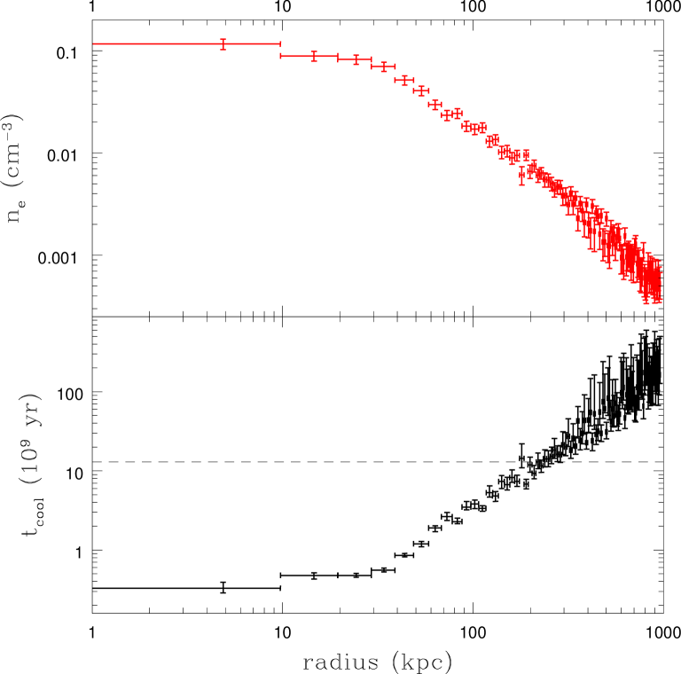
Figure 13: Electron density $n_{\rm e}$ and cooling time $t_{\rm cool}$ as a function of radius $r$. The cooling radius $r_{\rm cool}$ at which the cooling time profile becomes larger than the age of the universe $\frac{2}{3}\,$H${}_{0}=13\,$Gyr (dashed line) is $r_{\rm cool}\sim 230\,$kpc.

Figure 14: Entropy S as a function of radius. To guide the eye the entropy value for a temperature of 10 keV according to the numerical relation from Ponman, Cannon & Navarro (1999) has been plotted with dashed lines: S=567.0 at 0.1 virial radii, 0.1$\,c\,r_{\rm s}=257$ kpc (Sect. 5.1).

The fact that cooling times in the centres of cooling flow clusters are comparable to or even significantly less than the age of the universe is well known (Lea et al., 1973; Silk, 1976; Cowie & Binney, 1977; Fabian & Nulsen, 1977) and was an important motivation for the development of cooling flow models. In the next sections we explore the properties of such a cooling flow model for Abell 1835.

6.2 Standard cooling flow modelling and image analysis

In this section we report on the results from fitting cooling flow models to the spectra extracted from full circles centred on the geometrical cluster centre in the 0.5-7.0 keV band. In the standard cooling flow picture this yields the integrated mass deposition rate of the matter that cools out of the flow within a given radius.

We model the cooling flow using the RJCOOL emission model constructed according to the prescription in Johnstone et al. (1992) and include intrinsic absorption that may be acting on the cooling flow in the core of the cluster with a ZPHABS absorbing model (Balucinska-Church & McCammon, 1992) at the redshift of the cluster. We use the MEKAL plasma emission model (Kaastra & Mewe, 1993; Liedahl et al., 1995) to model the gravitational work done on the gas as well as emission of the intracluster gas outside the cooling flow:

$${\rm MODEL}_{2} = {\rm PHABS}_{\rm\,gal}\,\times\left[{\rm MEKAL}\,(T_{\rm high};Z;K)\frac{}{}\right.$$ (12)

$$\left.+\,{\rm ZPHABS}\,(\Delta N_{\rm H})\,\times\,{\rm RJCOOL}\,(\dot{M})\right].$$

The free parameters are given in brackets. The overall absorption in this model is fixed at the Galactic value (Dickey & Lockman, 1990). The intrinsic absorption $\Delta N_{\rm H}$ acts only on the cooling flow emission. The normalization of the cooling flow model, $\dot{M}$, measures the rate of gas cooling out of the flow. The other parameters of the cooling flow model, namely the metallicity $Z$ and upper temperature $T_{\rm high}$, are fixed to the values of the MEKAL component. This model is identical to model C in Allen (2000). It is a multi-phase model in the sense that at each radius all temperatures from the upper temperature down to the lowest temperature are present.

In Table 3 the results of the model fits are given for outer radii from 5 arcsec (25 kpc) to 50 arcsec (250 kpc). In Fig. 15 we have plotted with open circles the mass deposition results with an even finer spacing of the extraction circles. All of the fits are statistically acceptable, with reduced $\chi^{2}$ values around or slightly above unity. There is no significant improvement in $\chi^{2}$ over the simpler isothermal models eq. (1). The Chandra data for Abell 1835 cannot discriminate between single phase and multi-phase models.

Also shown in Fig. 15 (solid circles) is the mass deposition rate that may be deduced from the X-ray luminosity distribution (e.g., White et al., 1997) using our best-fit mass model from Sect. 5.1. It can be seen that the results from the spectral modelling and from the image analysis agree rather well out to 30 kpc, where the spectral mass deposition profile has a break at a mass deposition rate of 231${}^{+79}_{-53}\,M_{\odot}\,$yr^-1. The profile from the image analysis then itself has a break around 40 kpc. The solid line corresponds to a broken power-law fit to the mass deposition profile from the image analysis. Both profiles rise with a similar slope after their respective breaks, but disagree with respect to the amplitude. The spectral mass deposition profile rises up to a value of $\sim\,500\,M_{\odot}\,$yr^-1 within 250 kpc, whereas the profile from the image analysis rises to values of 1250 $M_{\odot}\,$yr^-1, which is consistent with the value from ROSAT (Allen, 2000).

Table 3: Cooling flow model fits (eq. (12)) to spectra from circular regions with radii $r$. We list the best-fit values for the model parameters mass deposition rate $\dot{M}$, upper temperature $T_{\rm high}$, metallicity $Z$ and intrinsic equivalent hydrogen column density $\Delta\,N_{\rm H}$. We also list the $\chi^{2}$ value, the number of degrees of freedom (DOF) and the reduced $\bar{\chi}^{2}$ value (see Table 1).

$r$ (kpc)	$\dot{M}$ ($M_{\odot}\,$yr-1)	kThigh (keV)	$Z$ (solar)	$\Delta N_{\rm H}$ (1022 cm-2)	$\chi^{2}$	DOF	$\bar{\chi}^{2}$
25	162.4${}^{+70.0}_{-57.9}$	4.8${}^{+0.9}_{-0.5}$	0.23${}^{+0.08}_{-0.07}$	0.20${}^{+0.10}_{-0.05}$	144.8	121	1.20
50	284.6${}^{+68.5}_{-93.2}$	4.9${}^{+0.2}_{-0.3}$	0.27${}^{+0.05}_{-0.04}$	0.31${}^{+0.13}_{-0.06}$	240.3	187	1.29
100	383.7${}^{+102.2}_{-99.7}$	6.3${}^{+0.4}_{-0.3}$	0.25${}^{+0.04}_{-0.04}$	0.26${}^{+0.09}_{-0.06}$	291.4	255	1.14
150	489.9${}^{+106.6}_{-122.1}$	7.1${}^{+0.4}_{-0.4}$	0.26${}^{+0.04}_{-0.03}$	0.20${}^{+0.06}_{-0.03}$	333.7	285	1.17
250	468.7${}^{+119.5}_{-119.9}$	7.5${}^{+0.4}_{-0.3}$	0.28${}^{+0.03}_{-0.04}$	0.23${}^{+0.07}_{-0.05}$	389.4	323	1.21

Figure 15: Integrated mass deposition rate $\dot{\rm M}$ as a function of radius $r$ determined spectrally (open circles) and from the image analysis (filled circles). The solid line is a broken power-law fit to the image analysis profile with a break at $r_{\rm break}=42$ kpc and exponents of 2.4 before and 0.4 after the break.

The intrinsic absorption $\Delta N_{\rm H}$ tabulated in Table 3 acting on the cooling flow emission rises from a mean equivalent hydrogen column density of $\Delta\,N_{\rm H}\sim\,0.2\,\times\,10^{22}\,$cm^-2 at a radius of 50 arcsec (250 kpc) by a factor of $\sim\,1.5$ when we look deeper into the cluster core. The statistical error bars on the intrinsic absorption are large, however. The temperature of the MEKAL component (which is linked to the upper temperature of the cooling gas) rises from about 5 keV in the centre to 9 keV within a circular aperture of 750 kpc radius.

6.3 Interpretation

6.3.1 A young central cooling flow?

Standard comoving multiphase cooling flow models (e.g., Nulsen, 1986) typically predict the profile of the mass deposition rate as a function of radius to be a power law. A break in the profile of the mass deposition rate, as seen in Fig. 15, may suggest that the flow mechanism is changing around the break radius. Allen et al. (2001b) interpret the presence of such breaks as an indicator of the age of the cooling flow, which they suggest is likely to be closely related to the time since the central regions of the cluster settled down following the last significant disruption by merger events or AGN activity. Given the cooling time at a radius of 30 kpc (Fig. 13), this would then limit the age of the cooling flow in Abell 1835 to be $\mathrel{\hbox{\hbox to0.0pt{\hbox{\lower 4.0pt\hbox{$\sim$}}\hss}\hbox{$<$}}}6{\times}10^{8}$ years.

The natural question which must be asked is whether such a young age for the cooling flow in Abell 1835 is plausible. Given the clear substructure observed in the core of the cluster (Sect. 3), some disturbance in the recent past seems likely. As discussed in Sect. 3, the small emission front seen in Fig. 4 to the south-east of the cluster core may have been caused by a cool, infalling gas cloud (e.g., see the work of  Markevitch et al., 2000). A 31.3 mJy FIRST radio source (Becker et al., 2000) is located in the cD galaxy. Although this source is relatively quiescent at present, it may have been much more powerful in the recent past and injected energy and momentum into the intracluster medium (possible problems with radio source heating are discussed by David et al. 2001 and Fabian et al. 2001). One should also recall that within the context of structure formation models, a cluster as hot and massive as Abell 1835, observed at a redshift $z\sim 0.25$, is highly unlikely to have formed more than a few Gyr before.

If the cluster remains undisturbed, the results on the cooling times and the mass deposition rate in Figs. 13 and 15 suggest that the core of the cluster will develop into a very massive cooling flow within a few Gyr. It is also possible that the cluster contained a large cooling flow before its most recent disturbance. Note that similar studies of the cooling flows in the Abell 2390 and 3C295 clusters indicate older ages of 2-3 and 1-2 Gyr, respectively.

We note that the fact that the break appears at a slightly smaller radius in the spectral analysis than the image analysis could simply be a consequence of the fact that although the gas starts to cool appreciably around 40 kpc, it has only had sufficient time to cool completely within $r\sim 30$ kpc. Note also that given the complex central morphology in Fig. 4, simple, spherically-symmetric cooling-flow models are unlikely to be applicable in detail.

As discussed by Allen et al. (2001a), in cases where the temperature of the cluster gas continues to rise beyond the outer edge of the cooling flow, spectral-measurements of the mass deposition rate covering regions larger than the cooling flow and using models similar to eq. (12), are likely to overestimate the true mass deposition rate. This is because the presence of relatively cool, ambient spectral components will tend to be modelled as part of a cooling flow. This situation is likely to have affected previous ASCA studies of the integrated cluster spectrum for Abell 1835 (Allen et al., 1996; Allen, 2000). We also note that the application of such models to large spatial regions may lead to the detection of low-temperature ‘cut-offs’ in the cooling flow spectra, which would simply be due to the fact that complete cooling occurs only within the innermost cooling flow proper.

6.3.2 XMM observations of Abell 1835

In a recent paper Peterson et al. (2001) present new results on grating spectra of Abell 1835 taken with the Reflection Grating Spectrometer (RGS) aboard the XMM-Newton X-ray observatory. They find no evidence for line emission from gas below 2.7 keV and, neglecting intrinsic absorption, place a 90 per cent confidence upper limit on the mass deposition rate from the cooling flow of $200\,\hbox{$\hbox{$\rm\thinspace M_{\odot}$}{\rm\thinspace yr}^{-1}\,$}$ for $H_{0}=70\hbox{$\hbox{${\rm\thinspace km}{\rm\thinspace s}^{-1}\,$}{\rm\thinspace Mpc}^{-1}$}$, $\Omega_{\rm m}=0.3$ and $\Lambda=0.7$. In fact, RGS has not found convincing evidence for a cooling flow in any galaxy cluster yet. Due to the inverse square dependence of the mass deposition rate on the luminosity distance, the RGS limit translates into $315\,\hbox{$\hbox{$\rm\thinspace M_{\odot}$}{\rm\thinspace yr}^{-1}\,$}$ for the $H_{0}=50\hbox{$\hbox{${\rm\thinspace km}{\rm\thinspace s}^{-1}\,$}{\rm\thinspace Mpc}^{-1}$}$ Einstein-de Sitter cosmology used here.

Overall, the RGS result for Abell 1835 implies a range of temperatures from 9 to 3 keV within the inner 0.5 arcmin radius (150 kpc), with the emission measures of that gas roughly matching a cooling flow. This is in agreement with our findings which show a radial gradient in the ambient gas temperature from ${\sim}8$ keV at 150 kpc to ${\sim}4\,$keV in the cluster core. In addition, we find evidence for complete cooling within the inner 30 kpc.

The RGS limit on the mass deposition is not easily reconciled with the large (${\dot{M}}\mathrel{\hbox{\hbox to0.0pt{\hbox{\lower 4.0pt\hbox{$\sim$}}\hss}\hbox{$>$}}}1000\,$$\hbox{$\rm\thinspace M_{\odot}$}{\rm\thinspace yr}^{-1}\,$) mass deposition rates inferred from previous studies of the integrated cluster spectrum observed with ASCA and ROSAT. Within the context of the young cooling flow model discussed above, however, the RGS results can be more easily accommodated. If one also accounts for the effects of intrinsic absorption, as required by the Chandra data, the apparent RGS limit of $315\,M_{\odot}\,$yr^-1 can be increased and is consistent with the Chandra result of 231${}^{+79}_{-53}\,M_{\odot}\,$yr^-1.

We note that the revised mass deposition rate of $\sim 200-300$ $\hbox{$\rm\thinspace M_{\odot}$}{\rm\thinspace yr}^{-1}\,$within $r\sim 30$ kpc in Abell 1835 is comparable to the optical star formation rate (normalized to the inferred number of A stars within the same region; Allen 1995; Crawford et al. 1999). Thus, it appears that a significant fraction of the material being deposited by the cooling flow within the central 30 kpc of Abell 1835 forms stars with a relatively normal IMF. Edge (2001) also reports the detection of a substantial molecular gas mass ($\sim 2\times 10^{11}$$\rm\thinspace M_{\odot}$) within the central regions of the cluster.

6.3.3 The origin of the temperature profile

The temperature profile in a cluster core is a result of the thermodynamic history of the intracluster gas. Chandra enables us for the first time to compare in detail the observed temperature profiles in clusters with those predicted by numerical studies of galaxy cluster formation (e.g., Eke, Navarro & Frenk, 1998; Frenk et al., 1999; Lewis et al., 2000; Pearce et al., 2000). In the studies by Eke et al. (1998) and Frenk et al. (1999), the temperature profiles of massive galaxy clusters (determined with smooth particle hydrodynamics, without including the effects of cooling), are often observed to drop slightly towards to core ($r\mathrel{\hbox{\hbox to0.0pt{\hbox{\lower 4.0pt\hbox{$\sim$}}\hss}\hbox{$<$}}}100$ kpc), then remain roughly constant on a plateau to $r\sim 1$ Mpc, before dropping again at larger radii.

Pearce et al. (2000) present temperature profiles for a sample of 20 simulated clusters, both with and without the effects of radiative cooling. For their largest cluster, the results obtained without including the effects of cooling are similar to those of Eke et al. (1998) and Frenk et al. (1999). However, when cooling is included, these authors find a “precipitous decline in temperature” in their largest cluster which they deem evidence for a cooling flow. The temperature profile for this cluster appears similar to that observed for Abell 1835 (Fig. 6). The work of Pearce et al. therefore suggests that the sharp temperature drops in the cores of cooling flow clusters (see also Allen et al., 2001a; David et al., 2001) could be due to the effects of radiative cooling over the lifetime of the cluster. Since in other simulations with cooling (e.g., Lewis et al., 2000) the temperature profile seems to keep rising with decreasing radius we note, however, that the effect of cooling in numerical simulations on the cluster temperature profiles does not seem to be entirely clear yet.

6.3.4 A massive cooling flow?

In this section we address whether an old ($\sim$5 Gyr), very massive ($\dot{M}\sim 1000\,M_{\odot}$ yr^-1) cooling flow, encompassing the entire central 150 kpc radius, can exist in Abell 1835. In this case, as mentioned in Sect. 6.3.2, our problem is to reconcile the large mass flow rate with the relatively small amount of X-ray line emission observed with RGS. Peterson et al. (2001) and Fabian et al. (2001) discuss a number of processes that may be relevant, two of which are investigated here.

The first model invokes an inhomogeneous distribution of metals that can be entered into XSPEC using the following prescription:

$${\rm MODEL}_{3}={\rm PHABS}_{\rm gal}\times$$

$$\left[{\rm MEKAL}\left(T_{\rm high};Z;K\right)+{\rm ZPHABS}\left({\Delta}N_{\rm H}\right)\times\right.$$

$$\left.\left({\rm RJCOOL}_{1}\left(\dot{M};Z=0\right)+{\rm RJCOOL}_{2}\left(0.1\,\dot{M};10{\times}Z\right)\right)\right]$$

where the free parameters (given in brackets) are the same as in eq. (12), but with the mass deposition rate distributed between two cooling flow components of which one has zero metallicity and the other all the heavy elements. This model describes a situation where most of the heavy elements are confined to small regions, so that the bulk of the cooling flow is extremely metal poor. The ratio of the mass of the metal poor and metal rich regions was fixed as 10:1. We have fitted this model to the Chandra spectrum extracted from a circle with a radius of 30 arcsec (150 kpc). The best-fit parameters are given in Table 4. The total mass deposition rate is 1070 $M_{\odot}$ yr^-1. Although the mass deposition rate is large, however, the emission lines due to cool gas are suppressed. The Fe XVII line at 15.01Å, for example, is suppressed by about a factor 4. However, the Fe XXII and Fe XXIII complex around 12.2 Å, which is strongly constrained by the RGS data, is only suppressed by a factor 2 by this model. This appears to be inconsistent with the RGS result.

Table 4: Best-fit parameters for possible massive cooling flow models. The upper limit on the metallicity in the first model was fixed to the software limit $Z=5$ in the high metallicity component.

model	Thigh (keV)	Tlow (keV)	$Z$ (solar)	$\Delta$N${}_{\rm H}\,(10^{22}\,{\rm cm}^{-2})$	$\dot{M}\,(M_{\odot}\,{\rm yr}^{-1})$	$\chi^{2}$	DOF	$\bar{\chi}^{2}$
inhomogeneous metallicities	11.0${}^{+2.3}_{-2.1}$	-	$0.50_{-0.08}$	0.08${}^{+0.02}_{-0.01}$	975.0${}^{+170.0}_{-148.0}$	322.3	285	1.13
absorbed cool gas	9.9${}^{+7.1}_{-2.0}$	2.6${}^{+0.7}_{-0.4}$	0.29${}^{+0.04}_{-0.04}$	0.51${}^{+0.15}_{-0.13}$	935.0${}^{+251.0}_{-187.0}$	331.7	284	1.16

The second model incorporates absorption that only acts on the gas below a certain temperature threshold and can be entered into XSPEC using the following prescription:

$${\rm MODEL}_{4}={\rm PHABS}_{\rm gal}\times$$

$$\left[{\rm MEKAL}\left(T_{\rm high};Z;K\right)+{\rm RJCOOL}_{1}\left(\dot{M};T_{\rm low}{\rightarrow}T_{\,\rm high}\right)+\right.$$

$$\left.{\rm ZPHABS}\left({\Delta}N_{\rm H}\right)\times\left({\rm RJCOOL}_{2}\left(\dot{M};0\,{\rm keV}{\rightarrow}T_{\,\rm low}\right)\right)\right].$$

Again, the model is very similar to the one presented in eq. (12). The best-fit values for the spectrum extracted from a circle with a radius of 30 arcsec (150 kpc) are also given in Table 4. The emission measure of gas below 2.7 keV is suppressed in the same way as the previous model, but this model also fails to adequately suppress the Fe XXII and Fe XXIII emission around 12.2 Å.

Although both models have significantly reduced emission from emission lines by cool ($\mathrel{\hbox{\hbox to0.0pt{\hbox{\lower 4.0pt\hbox{$\sim$}}\hss}\hbox{$<$}}}$ 2.7 keV) gas, their emission measure from gas at intermediate temperatures does not seem to be consistent with the RGS results.

7 Conclusions

We have presented the analysis of 30 ksec of Chandra ACIS-S3 observations of the galaxy cluster Abell 1835, of which 20 ksec were usable for spectroscopic analysis. Overall, the X-ray image shows a relaxed looking galaxy cluster. The X-ray isocontours in the centre are elliptical with an axis ratio of 0.85. In the inner 30 kpc radius, however, we detect clear substructure in the image.

Using isothermal fits to spectra from annular regions around the cluster centre we have measured the temperature, metallicity and photoelectric absorption of the cluster gas as a function of distance from the cluster centre. The temperature analysis reveals a steep drop in the temperature from 12 keV in the outer regions to only 4 keV in the cluster core. We also find evidence for a rise in the photoelectric absorption towards the cluster core, but no indication of a change in the metallicity with radius.

The Chandra data provide tight constraints on the gravitational potential of the cluster which can be parameterized by an NFW mass model. The best-fit NFW model has a scale radius $r_{\rm s}=0.64^{+0.21}_{-0.18}$ Mpc, an effective velocity dispersion $\sigma=1275\pm 160\,$km s^-1, a concentration parameter $c=4.0^{+0.54}_{-0.64}$ and a total mass $M=9{\times}10^{14}\,M_{\odot}$ within 1 Mpc. We measure the X-ray gas mass fraction of Abell 1835 as a function of radius and use this to deduce a cosmic matter density $\Omega_{\rm m}=0.40\pm 0.09\,h_{50}^{-0.5}$.

The projected mass within a radius of $\sim$150 kpc implied by the presence of gravitationally lensed arcs in the cluster is in good agreement with the mass models preferred by the Chandra data. This rules out any significant contributions from non-thermal sources of X-ray gas pressure (e.g., bulk motions, magnetic fields).

The detection of the Sunyaev-Zeldovich (SZ) effect (Sunyaev & Zeldovich, 1972) in Abell 1835 was recently reported by Mauskopf et al. (2000). The temperature (Fig. 8) and electron density (Fig. 13, upper panel) profiles determined in this paper can be used to predict the cosmology-dependent SZ effect in the cluster. This calculation and the cosmological implications of the SZ-detection by Mauskopf et al. (2000) are described elsewhere (Schmidt & Allen 2001, in preparation).

The Chandra data imply a radiative cooling time for the gas in the centre of Abell 1835 of about $3{\times}10^{8}$ yr. By fitting cooling flow models to spectra from circular regions around the cluster centre, we measure a mass deposition profile that can be represented by a broken power law with a break at a radius of 30 kpc, within which the integrated mass deposition rate is $231^{+79}_{-53}\,M_{\odot}$ yr^-1. We observe a similar behaviour in the mass deposition profile that can be derived from an image deprojection analysis, although the break in this case appears at a slightly larger radius $r\sim$40 kpc. The spectral and the imaging mass deposition profiles agree within $r\sim$30 kpc. If we associate the cooling time of the X-ray gas at the break radius with the age of the cooling flow (Allen et al., 2001b), we obtain an age of $\sim 6{\times}10^{8}$ yr.

Recent results from the XMM-Newton X-ray observatory (Peterson et al., 2001) limit the mass deposition rate in Abell 1835 to 315 $M_{\odot}\,$yr^-1, neglecting intrinsic absorption. This limit appears to be consistent with our result of having a young cooling flow with a mass deposition rate $\dot{M}=231^{+79}_{-53}\,M_{\odot}\,$yr^-1 in the centre of Abell 1835, particularly if one also includes the effects of intrinsic absorption as required by the Chandra data. The young cooling flow scenario is supported by the detection of substructure in the core, which shows that this region has not completely relaxed. Strong signs of star formation have been detected in the inner 30 kpc with optical spectroscopy (Allen, 1995) that could be fuelled by the inflowing gas.

References

- Allen (1995) Allen S.W., 1995, MNRAS 276, 947
- Allen (1998) Allen S.W., 1998, MNRAS, 296, 392
- Allen (2000) Allen S.W., 2000, MNRAS, 315, 269
- Allen et al. (2001a) Allen S.W., Ettori S., Fabian A.C., 2001a, MNRAS, accepted, preprint astro-ph/0008517
- Allen et al. (2001b) Allen S.W., Fabian A.C., Johnstone R.M., Nulsen P.E.J., Arnaud K.A., 2001b, MNRAS, accepted, preprint astro-ph/9910188
- Allen et al. (2001c) Allen S.W., et al., 2001c, MNRAS, accepted, preprint astro-ph/0101162
- Allen et al. (1992) Allen S.W., Edge A.C., Fabian A.C., Boehringer H., Crawford C.S., Ebeling H., Johnstone R.M., Naylor T., Schwarz R.A., 1992, MNRAS, 259, 67
- Allen et al. (1996) Allen S.W., Fabian A.C., Edge A.C., Bautz M.W., Furuzawa A., Tawara Y., 1996, MNRAS, 283, 263
- Arnaud (1996) Arnaud K.A., 1996, Astronomical Data Analysis Software and Systems V, eds. Jacoby G. and Barnes J., p17, ASP Conf. Series volume 101
- Balucinska-Church & McCammon (1992) Balucinska-Church M., McCammon D., 1992, ApJ, 400, 699
- Bartelmann (1995) Bartelmann M., 1995, A&A, 299, 11
- Bartelmann (1996) Bartelmann M., 1996, A&A, 313, 697
- Becker et al. (2000) Becker R.H., Helfand D.J., White R.L., Gregg M.D., Laurent-Muehleisen S.A., 2000, internet: sundog.stsci.edu
- Buote & Canizares (1996) Buote D.A., Canizares C.R., 1996, ApJ, 457, 565
- Crawford et al. (1999) Crawford C.S., Allen S.W., Ebeling H., Edge A.C., Fabian A.C., 1999, MNRAS, 306, 857
- Crawford et al. (2000) Crawford C.S., Fabian A.C., Gandhi P., Wilman R.J., Johnstone R.M., 2000, submitted to MNRAS, preprint astro-ph/0005242
- Cowie & Binney (1977) Cowie L.L., Binney J., 1977, ApJ, 215, 723
- David et al. (2001) David L.P., Nulsen P.E.J., McNamara B.R., Forman W., Jones C., Ponman T., Robertson B., Wise M., 2001, submitted to ApJ, preprint astro-ph/0010224
- Dickey & Lockman (1990) Dickey J.M., Lockman F.J., 1990, ARAA, 28, 215
- Dupke & White (2000) Dupke R.A., White R.E., 2000, ApJ, 528, 139
- Ebbels et al. (1998) Ebbels T., et al., 1998, MNRAS, 295, 75
- Ebeling et al. (1998) Ebeling H., Edge A.C., Bohringer H., Allen S.W., Crawford C.S., Fabian A.C., Voges W., Huchra J.P., 1998, MNRAS, 301, 881
- Edge et al. (1999) Edge A.C., Ivison R.J., Smail I., Blain A.W., Kneib J.-P., 1999, MNRAS 306, 599
- Edge (2001) Edge A.C., 2001, MNRAS, accepted, preprint astro-ph/0106225
- Eke et al. (1998) Eke V.R., Navarro J.F., Frenk C.S., 1998, ApJ, 503, 569
- Ettori & Fabian (1999) Ettori S., Fabian A.C., 1999, MNRAS, 305, 834
- Evrard (1997) Evrard A.E., 1997, MNRAS, 292, 289
- Fabian (1994) Fabian A.C., 1994, ARAA, 32, 277
- Fabian & Nulsen (1977) Fabian A.C., Nulsen P.E.J., 1977, MNRAS, 180, 479
- Fabian et al. (2000a) Fabian A.C., et al., 2000a, MNRAS, 315, L8
- Fabian et al. (2000b) Fabian A.C., et al., 2000b, MNRAS, 318, L65
- Fabian et al. (2001) Fabian A.C., Mushotzky R. F., Nulsen P. E. J., Peterson J. R., 2001, MNRAS, in press, preprint astro-ph/0010509
- Frenk et al. (1999) Frenk C.S., et al., 1999, ApJ, 525, 554
- Fukugita et al. (1998) Fukugita M., Hogan C.J., Peebles P.J.E., 1998, ApJ, 503, 518
- Johnstone et al. (1992) Johnstone R.M., Fabian A.C., Edge A.C., Thomas P.A., 1992, MNRAS, 255, 431
- Kaastra & Mewe (1993) Kaastra J.S., Mewe R., 1993, Legacy, 3, 16
- Kassiola & Kovner (1993) Kassiola A., Kovner I., 1993, ApJ, 417, 450
- Kayser & Schramm (1988) Kayser R., Schramm T., 1988, A&A, 191, 39
- Kneib (2000) Kneib J.-P. (PI), 2000, HST proposal 8249
- Kormann et al. (1994) Kormann R., Schneider P., Bartelmann M., 1994, A&A, 284, 285
- Kriss et al. (1983) Kriss G.A., Cioffi D.F., Canizares C.R., 1983, ApJ, 272, 439
- Lewis et al. (2000) Lewis G.F., Babul A., Katz N., Quinn T., Hernquist L., Weinberg D.H., 2000, ApJ, 536, 623
- Lea et al. (1973) Lea S.M., Silk J., Kellogg E., Murray S., 1973, ApJL, 184, 105
- Liedahl et al. (1995) Liedahl D.A., Osterheld A.L., Goldstein W.H., 1995, ApJ, 438, L115
- Madau et al. (1996) Madau P., Ferguson H.C., Dickinson M.E., Giavalisco M., Steidel C.C., Fruchter A., 1996, MNRAS, 283, 1388
- Markevitch et al. (1998) Markevitch M., Forman W.R., Sarazin C.L., Vikhlinin, A., 1998, ApJ, 503, 77
- Markevitch et al. (2000) Markevitch M., et al., 2000, ApJ, 541, 542
- Mason et al. (2001) Mason B.S., Myers S.T., Readhead A.C.S, submitted to ApjL, preprint astro-ph/0101170
- Mauskopf et al. (2000) Mauskopf P.D., et al., 2000, ApJ, 538, 505
- Navarro et al. (1997) Navarro J.F., Frenk C.S., White S.D.M., 1997, ApJ, 490, 493 (NFW)
- Nulsen (1986) Nulsen P.E.J., 1986, MNRAS, 221, 377
- O’Meara et al. (2000) O’Meara J.M., Tytler D., Kirkman D., Suzuki N., Prochaska J.X., Lubin D., Wolfe A.M., 2000, ApJ, submitted, preprint astro-ph/0011179
- Pearce et al. (2000) Pearce F.R., Thomas P.A., Couchman H.M.P., Edge A.C., 2000, MNRAS, 317, 1029
- Peterson et al. (2001) Peterson J., et al., 2001, A&A, 365, L104
- Press et al. (1992) Press W.H., Teukolsky S.A., Vetterling W.T., Flannery B.P., 1992, Numerical Recipes in C, 2nd edition, Cambridge Univ. Press, Cambridge
- Ponman et al. (1999) Ponman T.J., Cannon D.B., Navarro J.F., 1999, Nat, 397, 135
- Sarazin (1988) Sarazin C.L., 1988, “X-ray emission from clusters of galaxies”, Cambridge University Press, Cambridge
- Schneider et al. (1992) Schneider P., Ehlers J., Falco E.E., 1992, Gravitational Lensing, Springer Verlag, Berlin
- Schramm (1990) Schramm T., 1990, A&A, 231, 19
- Schramm (1994) Schramm T., 1994, A&A, 284, 44
- Silk (1976) Silk J., 1976, ApJ, 208, 646
- Smith et al. (2000) Smith G.P., Kneib J.-P., Ebeling H., Czoske O., Smail I., 2000, submitted to ApJ, preprint astro-ph/0008315
- Sunyaev & Zeldovich (1972) Sunyaev R., Zeldovich Y., 1972, Comments Astrophys. Space Phys., 4, 173
- Weisskopf et al. (2000) Weisskopf M.C., Tananbaum H.D., Van Speybroeck L.P., O’Dell S.L., 2000, SPIE 4012, 1, preprint astro-ph/0004127
- White et al. (1993) White S.D.M., Efstathiou G., Frenk C.S., 1993, MNRAS, 262, 1023
- White & Fabian (1995) White D.A., Fabian A.C., 1995, MNRAS, 273, 72
- White et al. (1997) White D.A., Jones C., Forman W., 1997, MNRAS, 292, 419