An Analysis of 900 Optical Rotation Curves:
The Universal Rotation Curve As A Power-Law
And The Development Of A Theory-Independent
Dark-Matter Modeller

Abstract

One of the largest $H_{\alpha}$ rotation curve data bases of spiral galaxies currently available is that provided by Persic & Salucci, (astro-ph/9502091) hereafter PS 1995, which has been derived by them from unreduced rotation curve data of 965 southern sky spirals obtained by Mathewson, Ford & Buchhorn, hereafter MFB 1992. Of the original sample of 965 galaxies, the observations on 900 were considered by PS 1995 to be good enough for rotation curve studies, and the present analysis concerns itself with these 900 rotation curves.

The analysis is performed within the context of the basic hypothesis that the phenomenology of rotation curves in the optical disc (that is, away from the dynamical effects of the bulge) can be systematically described in terms of a general power-law $V=A\,R^{\alpha}$, valid for $R\,>\,R_{min}$, where $R_{min}$ is an estimate of the transition radius between bulge-dominated and disc-dominated dynamics. The analysis begins by showing how this model provides an extremely good description of the generic behaviour of rotation curves in the optical disc and, furthermore, how it imposes very detailed correlations between the free parameters, $A$ and $\alpha$, of the model.

These correlations are investigated, and shown to imply, via first and second-order models, a third-order model according to which the rotation velocity, $V$, at any radial displacement in the optical disc of any given spiral galaxy is given by $V/V_{0}=(R/R_{0})^{\alpha}$, where $R_{0}>R_{min}$, and $V_{0}$ are given as approximate functions of the galaxy’s absolute magnitude and surface brightness whilst $\alpha$ is an unidentified function of other galaxy parameters - of which the most significant ones will be the relative proportions of the disc, bulge and halo mass-components. It is this latter function which provides the opportunity for a dark-matter modelling process which is independent of any particular dynamical theory.

Furthermore, it is shown that the conclusion of PS 1986, that optical-disc dynamics contain no signature of the transition from disc-dominated dynamics to halo-dominated dynamics, is extremely strongly supported by this analysis.

1 Introduction

It has been know for several years - for example, Rubin, Burstein, Ford & Thonnard, hereafter RBFT - that optical rotation curve shapes are strongly determined by luminosity in the sense that, within any given morphological class and away from the innermost part of the rotation curve, high luminosity galaxies have almost flat rotation curves, whilst low luminosity galaxies have more ‘rounded and rising’ rotation curves.

However, until recently all studies of the correlations existing between rotation curve kinematics and global galaxy properties have necessarily been confined to relatively small samples of rotation curves, and have therefore been subject to the corresponding uncertainties. This problem has been rectified by the publication of 900 good quality rotation curves by PS 1995. A first analysis of this data was given by Persic et al (1996), hereafter PSS, in which they concluded that there exists a ‘universal rotation curve’ for spiral galaxies which is determined primarily by the total luminosity of the galaxy concerned, and the essence of this conclusion is confirmed here. The present analysis of the same data differs crucially from that of PSS in that an early decision was taken to analyse the data within the context of the hypothesis that rotation curves in the optical disc (that is, away from the dynamical effects of the bulge) could be reasonably described by a generalized power law, $V_{rot}=A\,R^{\alpha}$, where $R\,>\,R_{min}$ and $R_{min}$ represents an estimate of the transition radius from bulge-dominated to disc-dominated dynamics. This decision, which was motivated by arguments which are independent of the matters at hand, could easily have resulted in relative failure in the sense of providing no particular insights into rotation curve structure. In fact, the opposite happened and it was found that the hypothesis imposes extremely strong correlations between rotation curve kinematics, total luminosities and surface brightnesses, thereby giving a detailed confirmation to the general thrust of the PS studies, and a strong confirmation to the particular idea of the universal rotation curve.

In detail, the primary conclusion of this analysis is that the rotation curve in the optical disc of any given spiral galaxy with absolute magnitude $M$ and surface brightness $S$ behaves according to

$${V\over V_{0}} = \left({R\over R_{0}}\right)^{\alpha},$$ (1)

$$\log V_{0} \approx -0.584-0.133\,M-0.000243\,S,$$

$$\log R_{0} \approx -3.291-0.208\,M-0.00292\,S,$$

$$\alpha \approx g(d_{m},\,b_{m},\,h_{m}),$$

where $g(d_{m},\,b_{m},\,h_{m})$ is some undetermined function for which the most significant parameters are probably the disc-mass ($d_{m}$), bulge-mass ($b_{m}$) and halo-mass ($h_{m}$) respectively. Since this model is shown to account for over 90% of the variation in the pivotal diagram (equivalent to a regression correlation of 0.95), it can be considered as, at the very least, an extremely good approximation to the statistical reality, as judged for a large number of spiral discs.

The best model that can be given for the undetermined exponent, $\alpha$, in terms of the data provided by PS 1995 is that $\alpha=2.56+0.105\,M$, which accounts for over 29% of the variation in the $(\alpha,\,M)$ plot (equivalent to a regression correlation of 0.55). We see immediately from this model that high luminosity galaxies are the ones which possess the flattest rotation curves, whilst the low luminosity galaxies are the ones which possess the ‘rounded and rising’ rotation curves - thereby confirming the RBFT result for a very large sample.

A further, and very significant, consequence of the success of (1) is its implied confirmation of the PS 1986 result that optical discs appear to contain no signature of the transition from disc-dominated dynamics to halo-dominated dynamics. PS reached this conclusion after an analysis of 42 rotation curves showed the near-constancy, over the whole of each optical rotation curve, of the parameter ${\hat{V}}\equiv(\Omega-K/2)R$, for angular velocity $\Omega$ and epicyclic frequency $K$. The connection between this result of PS and the present perspective is discussed in Appendix A.

Further evidence supporting the apparent absence of any kinematical transition region in the optical disc arises through the discovery of very strong correlation between $R_{opt}$ and $R_{min}$, where $R_{min}$ is a theory-independent estimate of the transition region between bulge-dominated and disc-dominated dynamics (see Appendix B). The existence of such a correlation implies a causal connection between $R_{min}$ and $R_{opt}$ which, again, argues against the existence of sharply delineated transition regions between disc-dominated and halo-dominated dynamics.

Finally, and of potentially greatest significance, it is to be noted that halo-mass only enters the system through the undetermined function $\alpha$; this fact provides the possibility of a dark-matter modelling process which is independent of any particular dynamical theory. Specifically, since, for any given galaxy, reasonable estimates for $d_{m}$ and $b_{m}$ can be obtained, then it becomes possible to model $\alpha$ in terms of these two quantities. Analysis of any systematic differences arising between $\alpha$-values calculated from the rotation curves, and the modelled $\alpha$-values, will then, in principle, allow systematic estimates of any given galaxy’s dark-matter content to be given in terms of the galaxy’s disc-mass, bulge-mass and surface brightness.

2 The Data

The data given by PS is obtained from the raw $H\alpha$ data of MFB by deprojection, folding and cosmological redshift correction. For any given galaxy, the data is presented in the form of estimated rotational velocities plotted against angular displacement from the galaxy’s centre; estimated linear scales are not given and no data-smoothing is performed.

The analysis proposed here requires the linear scales of the galaxies in the sample to be defined which, in turn, requires distance estimates of the sample galaxies from our own locality. This information is given in the original MFB paper in the form of three variations of the Tully-Fisher, hereafter TF, distance estimate, say TF1, TF2 and TF3. TF1 is derived by using the TF relation for Fornax obtained from magnitude data; TF2 is the Malmquist-bias corrected form of TF1 giving TF2=1.08$\times$TF1 for all galaxies; TF3 is obtained by using the TF relation for Fornax obtained from rotation curve data. The current analysis is based upon TF3.

Table 3 gives the morphological type-distribution in the PS 1995 data base, and shows that the great majority of the selected galaxies are of types 3,4,5 and 6, with only two examples of types 0,1,2 and a tail of 31 examples of types 7,8,9.

Table 3
Galaxy	Sample
Type	Size
0,1,2	2
3	306
4,5	177
6	384
7,8,9	31

For the purposes of the following analysis, no distinction is made between type classes, and so the whole sample of 900 rotation curves is used. However, the results of this analysis remain unchanged, except in the numerical details, when it is repeated on any of the subsets consisting of types $\left\{3\right\}$, $\left\{4,5\right\}$ or $\left\{6\right\}$.

The details of the data-reduction used in these analyses are given in Appendix B and, briefly, they amount to a prior-decided means of minimizing the effect of the bulge on the rotation-curve calculations.

3 A Necessary Condition For The Power-Law Hypothesis

Suppose the power-law hypothesis of (1) to be true; in this case, and excepting for the inevitable high level of noise, a plot of any given rotation curve in the $(\log R,\,\log V)$ plane would lie on a straight line. Since the rotation curves are not identical then, for the 900 rotation curves, we would obtain 900 distinct straight-line plots in the $(\log R,\,\log V)$ plane. In the following, we show that, in this case, the mean plot of the 900 separate plots must also be a straight line: For a given $\log R$, the corresponding $\log V$ value for each of the 900 rotation curves would be given by

$$\log V_{k}=a_{k}+b_{k}\,\log R,~{}~{}k=1..900.$$

Summing over $k$, and forming the mean response, we find

$${\rm Mean}\left(\log V\right)=A+B\,\log R,$$

so that, as stated, the mean plot is also a straight line. It follows that a necessary condition for optical rotation curve data to be described by a power law is that the mean plot of all the rotation curves in the $(\log R,\,\log V)$ plane must be a (statistically) straight line. So, the strategy of the initial analysis is described as follows:

• Reduce all the data in the combined sample of 900 rotation curves to a uniform linear scale based on TF3;

• Superimpose all the data of the combined sample into a single data set;

• Divide the data set into bins subject to some convenient criteria. For present purposes, the bin-width was chosen as $0.057kpc$ subject to the constraint that each bin contained at least 200 data points. In practice, the average per bin is about 800 data points.

• Form the average of the data in each bin and plot it.

The rationale is simply that, if the power law hypothesis is correct, then the internal noise on the data for the 900 separate rotation curves should largely cancel out over the averaging process. The result is plotted in Figure 1 - and it is to be emphasized that this plot does not represent a physical rotation curve, but is merely a convenient graphic tool designed to illustrate a statistical point.

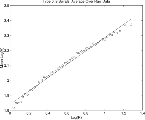
Figure 1: Mean Of 900 Individual Rotation Curves

The only discernible sense of any possible systematic deviation from a purely linear behaviour occurs in the innermost part of the plot; apart from this, the figure provides solid support for the idea that a general power law is, at the very least, a good working approximation to $H_{\alpha}$ rotation curve data, and provides the necessary rationale for the basic analysis of this paper.

4 The Minimization Of Bulge-Dominated Dynamics In Rotation Curve Data

Before beginning the analysis proper, we note that the apparent deviation from linear behaviour on the innermost part of the rotation curve, noted in the previous section, is easily understood in terms of the transition from bulge-dominated to disc-dominated dynamics. In this section, we describe the effect of implementing the data-reduction process described in Appendix B which is designed to minimize the effects of bulge-dominated dynamics in the present considerations . In effect, this process is a numerical process which removes the innermost data points on any given rotation curve according to how statistically ‘unusual’ those points are in relation to the rest of the data, and its effects are described below in Figures 2 & 3 and in Tables 1 & 2.

Figure 2 plots the measured $R_{min}$ against the measured $R_{opt}$ before any data reduction is performed, whilst Figure 3 plots the calculated $R_{min}$ arising from the data reduction process against the measured $R_{opt}$. It is clear from these diagrams that the data reduction process reveals a fairly strong correlation between $R_{min}$ and $R_{opt}$. The change between the two diagrams is quantified in Tables 1 & 2.

Table 1
$R_{opt}=b_{0}+b_{1}\,R_{min}$
Before data reduction
Predictor	Coeff	Std Dev	t-ratio	p
Const.	7.25	0.13	57	0.00
$R_{min}$	1.62	0.11	14	0.00
$R^{2}$  =  19.2%
Table 2
After data reduction
Predictor	Coeff	Std Dev	t-ratio	p
Const.	5.73	0.14	41	0.00
$R_{min}$	1.64	0.07	24	0.00
$R^{2}$  =  38.6%

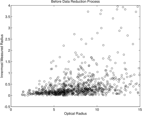
Figure 2: Before Data Reduction

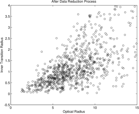
Figure 3: After Data Reduction

It is surprising to note that Table 1 clearly shows that $R_{min}$ in the unreduced data is already a very significant (if very noisy) predictor for $R_{opt}$. However, after the data reduction process, both the significance and the reliability of $R_{min}$ as a predictor for $R_{opt}$ increase considerably.

If we consider the post data-reduction values of $R_{min}$ as strong predictors of bulge-radius (which is reasonable), then the strong post data-reduction correlation between $R_{min}$ and $R_{opt}$ can be seen as a correlation between bulge radius and optical disc radius. The fact that a significant correlation between $R_{min}$ and $R_{opt}$ already existed prior to the data reduction can then be interpreted to indicate that the pre data-reduction $R_{min}$ values were already significant (if very noisy) predictors of bulge-radius.

There is a further significant implication of the strong post data-reduction correlation between $R_{min}$ and $R_{opt}$: the correlation implies a strong causal connection between the two values which, in turn, implies that any effect the halo has on $R_{opt}$ is necessarily balanced by a corresponding effect of the halo on $R_{min}$. In particular, the correlation is inconsistent with the existence of any strong transition region between disc-dominated and halo-dominated dynamics in the optical disc - a conclusion already reached by PS 1986, and others and clear from Figure 1.

5 A Basic Correlation Imposed By Power-Law Rotation Curves

In the following, it is shown that an extremely strong correlation exists between the power-law parameters over the whole PS sample, and the correlation is detected in the following way:

• The basic assumption is that rotation velocities behave as $V=AR^{\alpha}$ so that $\log V=\log A+\alpha\,\log R$;

• For each of the 900 rotation curves in the sample, regress $\log V$ on $\log R$ to obtain estimates of $\log A$ and $\alpha$;

• Plot the 900 pairs $(\alpha\,,\log A)$ on a single diagram.

The results of this exercise are shown in Figure 4,

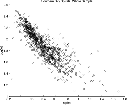
Figure 4: $(\alpha,\log A)$ plotted for each of 900 rotation curves

and shows that there exists an extremely strong negative $(\alpha,\log A)$ correlation. The only obvious deviations from what could be called an almost perfect linear correlation are, firstly, a slight hint of curvature along the lower boundary of the distribution and, secondly, the fan-like behaviour of the diagram going from a broad spread of points at the bottom right-hand of the figure to a narrow neck at the top left-hand of the figure.

In the following sections, we show that the structure of Figure 4 orders the galaxies in the sample according to their absolute magnitude and surface brightness properties.

6 The First-Order 70% Model

6.1 The Basic Analysis

The first-order model simply assumes that the $(\alpha,\log A)$ relationship underlying Figure 4 is linear, so that

$$\log A=a_{0}+b_{0}\alpha,$$ (2)

where $a_{0}$ and $b_{0}$ are constants, and linear regression shows that this model can account for 70% of the variation (equivalent to a regression correlation coefficient of 0.84) in Figure 4.

6.2 Geometric Implications

It is easily shown that when the parameters, $(m,c)$, of a set of lines $y=mx+c$ in the $(x,y)$-plane are constrained to satisfy $c=y_{0}-x_{0}m$, for constants $(x_{0},y_{0})$, then the lines themselves are constrained to meet at the fixed point $(x_{0},y_{0})$ in the plane. Consequently, in the present context, the first-order linear approximation (2) implies that all rotation curves,

$$\log V=\log A+\alpha\log R,$$ (3)

for which $\log A$ and $\alpha$ are related by (2), intersect at the fixed point $(-b_{0},a_{0})$ in the $(\log R,\log V)$ plane. If this fixed point is denoted as $(\log R_{0},\log V_{0})$, then (2) is more transparently written as

$$\log A=\log V_{0}-\alpha\log R_{0}$$ (4)

so that (3) implies

$$V=V_{0}\left({R\over R_{0}}\right)^{\alpha}.$$ (5)

Assuming the model (4), a linear regression on the data of Figure 4 subsequently gives $(\log R_{0},\,\log V_{0})\approx(0.84,2.22)$. Whilst the idea of a single intersection point for all rotation curves in the sample seems rather extreme, it is unambiguously deduced as a consequence of the first-order modelling of Figure 4 - and is therefore to be seen as a first-order approximation of the reality.

In the following sections, we give two powerful illustrations of the reality of the idea that optical rotation curves can be considered, in the first approximation, to converge in a very small region of the $(\log R,\,\log V)$ plane.

6.3 The Intersection Frequency
Diagram

A direct illustration of rotation curve convergence is given as follows: we have calculated the coordinates of intersection between all possible pairs of 200 randomly sampled rotation curves drawn from the full sample, and have plotted the frequencies of intersection along the $\log R$ and $\log V$ axes respectively in Figures 5 & 6.

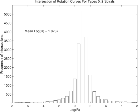
Figure 5: Frequency of Intersections on $\log R$ axis

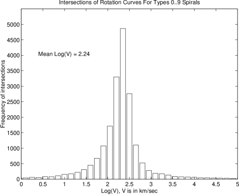
Figure 6: Frequency of Intersections on $\log V$ axis

It is clear from these figures that there is a very sharp peak of intersection points in both diagrams. Using the mean points in each diagram, together, they are consistent with a peak intersection point at $(\log R,\log V)\approx(1.02,2.24)$.

6.4 A Geometric Illustration Of Rotation Curve Convergence

A second, and dramatic, illustration of rotation curve convergence can be formed from the realization that, if the rotation curves really do converge on a single fixed point in the $(\log R,\log V)$ plane, then all of the rotation curves will transform into each other under rotations about the fixed point, $(\log R_{0},\log V_{0})$, in this plane.

This idea can be tested in the following way: suppose that an arbitrarily chosen straight line passing through the point $(\log R_{0},\log V_{0})$ is defined as a standard ‘reference line’. Since, according to the first-order model interpretation of Figure 4, all the rotation curves in the sample pass through the point $(\log R_{0},\log V_{0})$, then every rotation curve in the sample can be transformed into the standard reference line by a simple bulk-rotation about $(\log R_{0},\log V_{0})$. Since, according to this idea, the rotation curves are reduced to equivalence by the rotation, then the process of forming an ‘average rotation curve’ from the set of rotated such curves should greatly reduce the internal noise associated with the individual rotation curves, and we would expect the resulting average curve to be a very close fit to the standard reference line, referred to above.

In the following analysis, which is performed for all 900 galaxies in the sample, the technique described in Appendix C is used to refine the histogram estimate of $(1.02,2.24)$, given in the last section, to the optimal value for the fixed point as $(\log R_{0},\,\log V_{0})=(1.06,2.29)$.

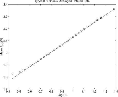
Figure 7: Types 0..9 spirals; Averaged rotated data

The solid line in Figure 7 is the standard reference line which is defined to pass through the fixed point $(\log R_{0},\,\log V_{0})=(1.06,2.29)$, and fixed arbitrarily so that $\log A=1.5$. The results are not sensitive to the choice of this latter parameter. The circles in the figure show the results of rotating the 900 rotation curves of the sample about the fixed point so that they coincide in a least-square sense with the standard reference line, and then averaging over all the rotation curves. Each circle represents an average of approximately 800 separate measurements.

When Figure 7 is compared with Figure 1, we see that virtually all of the scatter present within the latter figure is eliminated in Figure 7, thereby providing the strongest possible evidence for the idea of the equivalence of rotation curves with respect to rotation about particular fixed points in the $(\log R,\log V)$ plane.

6.5 A Comparison of Three
$(\log R_{0},\,\log V_{0})$ Estimates

As we pointed out in §6.1, the first-order approximation of the $(\alpha,\,\log A)$ plot of Figure 4 implies directly that all $H_{\alpha}$ rotation curves pass through a single fixed point in the $(\log R,\,\log V)$ plane, and we have three distinct ways of estimating the position of this fixed point. The first way was by a direct linear regression on the data of Figure 4, the second way was by estimating the peaks of the intersection histograms of Figures 5 and 6 respectively, whilst the third way was by the minimization procedure described in §6.4 the results of which are shown in Figure 7. The three estimates are shown together in Table 4.

Table 4
Method	$\log R_{0}$	$\log V_{0}$
Regression	0.84	2.22
Mean Values	1.02	2.24
Minimization	1.06	2.29

There is clearly a high degree of consistency between the three methods which serves to emphasize the reality of the first-order effect.

7 The Second-Order 85%
Model

7.1 The Basic Analysis

Whilst, so far, Figure 4 has been analysed on the basis of a first-order linear model, there is the possibility that systematic internal structure exists in Figure 4. In this section, we show how the existence of this internal structure is strongly supported on the data, and leads to a second-order model which accounts for over 85% of the variation (equivalent to a regression correlation coefficient of 0.92) in the pivotal diagram, Figure 4.

Table 5
$(\alpha,\,\log A)$ data averaged in
magnitude-limited quartiles
Sample	Mean	Mean	Mean
Size	abs(mag)	$\alpha$	$\log A$
224	-22.20	0.22	2.15
227	-21.16	0.34	1.96
224	-20.27	0.47	1.79
225	-18.80	0.58	1.65

We begin by taking the 900 pairs of $(\alpha,\log A)$ data which form the basis of Figure 4 and partition them as near as possible into quartiles according to absolute magnitude; thus the data is partitioned into the brightest 25% of the sample, the next brightest 25% and so on. For each quartile, we then form the mean values of the absolute magnitude, $\log A$ and $\alpha$ respectively, and the results of this exercise are listed in Table 5 and plotted in Figure 8.

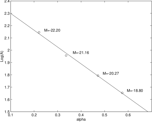
Figure 8: $(\alpha,\log A)$ data averaged in magnitude-limited quartiles

The solid line in the figure is the linear regression line fitted to the four data points, and the whole diagram can be considered as a condensed representation of the data plotted in Figure 4 showing the variation of absolute magnitude through that data. It is clear from Table 5 and Figure 8 that $\alpha$ and $\log A$ are each very strongly correlated with the absolute magnitude, thereby justifying a more detailed investigation.

7.2 The Refined Analysis

We begin by plotting the $(\alpha,\,\log A)$ data for each of these magnitude-limited quartiles and displaying these plots in Figure 9.

Figure 9: $(\alpha,\,\log A)$ plotted for each magnitude-limited quartile

Viewed collectively, the four diagrams of this figure display three significant features:

• Firstly, the diagram corresponding to the brightest magnitude-limited quartile shows that $(\alpha,\,\log A)$ data exhibits almost scatter-free linear behaviour, whilst the data of the remaining quartiles exhibits increasing scatter as absolute magnitude increases.

• Secondly, apart from this scatter, there appears to be a systematic variation of the data through the four diagrams when they are viewed in order of increasing absolute magnitude.

• Thirdly, the scatter evident in Figure 4 is seen to be a function of increasing absolute magnitude which, at face value, would suggest it is a function of increasing measurement uncertainties at the dimmer end of the sample. However, there is a feature which suggests that the situation is not this straightforward: specifically, the lower boundary of points in each diagram of Figure 9 is very sharply delineated whilst it is the upper boundary which becomes increasingly diffuse in the higher magnitude quartiles. If measurement uncertainty is the basic cause of scatter in these diagrams, then it is not immediately obvious why the lower boundary of points in every quartile is sharply delineated.

The reality of a systematic variation with increasing magnitude in the diagrams of Figure 9 is confirmed by forming the linear regression of $\log A$ on $\alpha$ for the data of each of these diagrams so that, for each diagram, there is a linear model analogous to (4). The results are listed in Table 6 and plotted in Figure 10. The figure shows very clearly that the four regression lines meet in a very small neighbourhood of the point $(0.9,1.5)$ of the $(\alpha,\,\log A)$ plane.

Table 6
$\log A=\log V_{0}-\alpha\,\log R_{0}$
Sample	$\log V_{0}$	$\log R_{0}$	Mean $M$
Size			of quartile
224	2.35	0.90	-22.20
227	2.23	0.80	-21.16
224	2.10	0.65	-20.27
225	1.89	0.41	-18.80

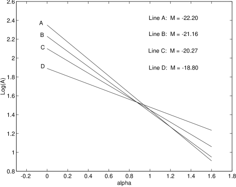
Figure 10: Regressions on $(\alpha,\,\log A)$ data in magnitude-limited quartiles

We have already noted that, when a set of lines $y=mx+c$ in the $(x,y)$-plane are constrained to meet at a fixed point, $(x_{0},y_{0})$ say, then the parameters $(m,c)$ of the lines are constrained to satisfy $c=y_{0}-x_{0}m$. In the present case, representing any of the lines in Figure 10 as $\log A=\log V_{0}-\alpha\,\log R_{0}$, this means that the parameters $(\log R_{0},\,\log V_{0})$ are constrained to satisfy $\log V_{0}\approx 1.5+0.9\,\log R_{0}$. Since, in Figure 10, the only thing which varies between the lines is the absolute magnitude, then we can expect $\log V_{0}$ and $\log R_{0}$ to be individual functions of absolute magnitude and this is confirmed by Table 6. Linear regression of the data of this table gives

$$\log V_{0} = -0.67-0.14\,M,$$ (6)

$$\log R_{0} = -2.34-0.15\,M$$

from which we get $\log V_{0}=1.51+0.93\,\log R_{0}$, which confirms the result obtained directly from Figure 10. We now note that the constants and coefficients in (6) can be ‘fine tuned’ in the following way: If we substitute equations (6) into (4) we obtain the relationship

$$\log A = \log V_{0}-\alpha\,\log R_{0}~{}~{}\rightarrow$$

$$\log A = -0.67-0.14\,M$$ (7)

$$+ 2.34\,\alpha+0.15\,\alpha\,M,$$

which shows directly that the model (6) is equivalent to a model for $\log A$ expressed in terms of $M$, $\alpha$ and $\alpha\,M$. Given this model for $\log A$, its coefficients can be optimised in a least-square sense by regressing $\log A$ directly on the predictors $M$, $\alpha$ and $\alpha\,M$ over the whole data set. This process gives

$$\log A = -0.56-0.13\,M$$

$$+ 2.27\,\alpha+0.14\,\alpha\,M,~{}~{}\rightarrow$$

$$\log A = \log V_{0}-\alpha\,\log R_{0},~{}~{}{\rm where}$$

$$\log V_{0} = -0.56-0.13\,M,$$

$$\log R_{0} = -2.27-0.14\,M.$$

with very strong statistics on the constant and coefficients, and shows that this regression accounts for over 85% of the variation (equivalent to a regression correlation coefficient of 0.92) in the pivotal diagram, which is Figure 4. A comparison with (7) shows only minor adjustments to the constants and coefficients of the $(\log R_{0},\,\log V_{0})$ models. Consequently, and using (5), the optimised second-order model gives the universal rotation curve as

$${V\over V_{0}} = \left({R\over R_{0}}\right)^{\alpha},$$ (8)

$$\log V_{0} = -0.56-0.13\,M,$$

$$\log R_{0} = -2.27-0.14\,M.$$

8 The Third-Order 90% Model

It has been shown that over 85% of the variation in the pivotal diagram, Figure 4, is accounted for by the second-order model (8) which depends only on absolute magnitudes. However, the PS data-base for the 900 rotation curves also provides estimates to the optical radius, $R_{opt}$, which, with the absolute magnitudes, allows us to estimate the surface brightness of each galaxy in the sample; since this represents independent information, it seems sensible to consider the effect of its inclusion in the model and, for present purposes, we define it to be in solar luminosities per square parsec so that

$$S\approx\left({2.5^{5-M}\over\pi R_{opt}^{2}}\right).$$

The second-order model, (8), was arrived at by initially noting that Table 6 implied the relations (6) which, in conjunction with the basic relationship $\log A=\log V_{0}-\alpha\,\log R_{0}$, allowed the deduction of the structure

$$\log A=a_{0}+a_{1}\,\alpha+a_{2}\,M+a_{3}\,\alpha\,M$$

for the $\log A$ model. If (8) is to be modified by the introduction of $S$, so that

$$\log V_{0}=b_{0}+b_{1}\,M+b_{2}\,S$$

$$\log R_{0}=c_{0}+c_{1}\,M+c_{2}\,S,$$

then the $\log A$ model will have the structure

$$\log A = b_{0}+b_{1}\,M+b_{2}\,S$$ (9)

$$- c_{0}\,\alpha-c_{1}\,\alpha\,M-c_{2}\,\alpha\,S.$$

The results of regressing $\log A$ on the predictors $M$, $S$, $\alpha$, $\alpha\,M$ and $\alpha\,S$ are given in Table 7.

Table 7
$\log A=b_{0}+b_{1}\,M+b_{2}\,S-c_{0}\,\alpha-c_{1}\,\alpha\,M-c_{2}\,\alpha\,S$
Pred	Coeff	Std Dev	t-ratio	p
	$\times\,10^{4}$	$\times\,10^{4}$
Const.	-5840	890	-7	0.00
$M$	-1330	44	-30	0.00
$S$	-2.434	0.77	-3	0.00
$\alpha$	32910	1600	21	0.00
$\alpha\,M$	2080	84	25	0.00
$\alpha\,S$	29.23	2	14	0.00
$R^{2}~{}=~{}90.3\%$

This model now accounts for marginally over 90% of the variation (equivalent to a regression correlation coefficient of 0.95) in the pivotal diagram, Figure 4, and we see from the t-ratios that the surface brightness is most certainly a significant component of the model. Interpreting the table according to the model

$$\log A=\log V_{0}-\alpha\,\log R_{0},$$

$$\log V_{0}=b_{0}+b_{1}\,M+b_{2}\,S,$$

$$\log R_{0}=c_{0}+c_{1}\,M+c_{2}\,S,$$

we arrive, finally, at the third-order model

$${V\over V_{0}} = \left({R\over R_{0}}\right)^{\alpha},$$ (10)

$$\log V_{0} = -0.584-0.133\,M-0.000243\,S,$$

$$\log R_{0} = -3.291-0.208\,M-0.00292\,S.$$

Referring to Table 7 again, we see that $S$ is a very strong predictor for $\log R_{0}$, whilst its effect on $\log V_{0}$, whilst significant, is much less so. This conclusion is supported by numerical experimentation which shows that it can be omitted from $\log V_{0}$ with hardly any effect on the model. However, Table 7 shows that it probably is a real predictor for $\log V_{0}$, and so it is retained in the model.

8.1 A Secondary Test Of The Model

A secondary test of the validity of the third-order model can be given as follows: For each galaxy we compute $(R_{0},V_{0})$ according to (10), form the scaled profile $(R/R_{0},\,V/V_{0})$ and regress $\log(V/V_{0})$ on $\log(R/R_{0})$. If (10) is good enough, then the regression constant should be statistically zero. The distribution of the 900 regression constants is shown in Figure 11, for which a one-parameter t-test gives the 95% confidence interval for the mean of the distribution as $(-0.003,+0.007)$ whilst the 99.999% confidence interval is given as $(-0.010,+0.014)$. Thus, for all practical purposes, the regression constant can be considered as statistically zero, thereby confirming the quality of the model.

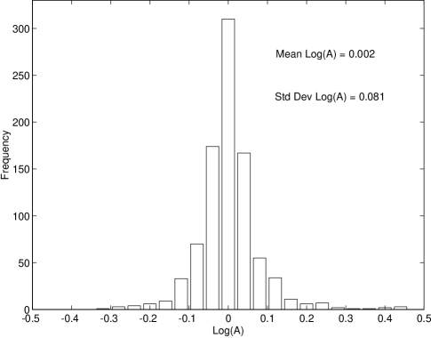
Figure 11: Distribution of 900 regression constants

8.2 The Brightest Quartile

Finally, as a means of demonstrating that the (already small) scatter about the zero point evident in Figure 11 is a function of uncertainty in the data, rather than due to a poor fit of the basic power-law model, we apply the third-order model directly to the 224 rotation curves of the brightest quartile, for which the $(\alpha,\,\log A)$ data is plotted in the first diagram of Figure 9. For this data, the distribution of the 224 regression constants arising from the linear regression of $\log(V/V_{0})$ data on $\log(R/R_{0})$ data is given in Figure 12.

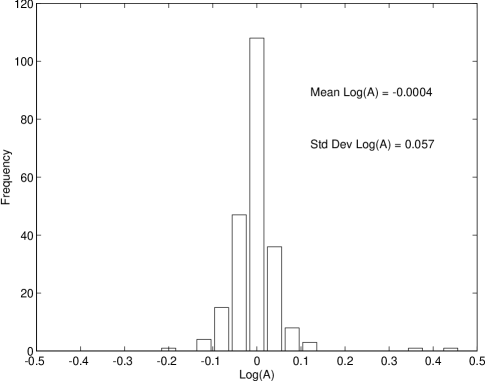
Figure 12: Brightest quartile regression constants

A direct visual comparison with Figure 11 shows immediately that the scatter of points about the zero point is very much reduced in the brightest quartile data, thereby supporting the hypothesis that the scatter which exists in Figures 11 and 12 is due purely to uncertainty in the data, and not at all due to any lack of fit of the general power-law model.

8.3 The Surface-Brightness Cut-Off

It has already been noted that the lower boundary of points in each of the magnitude-limited quartile plots of $(\alpha,\,\log A)$ shown in Figure 9 is very sharply delineated, whilst the corresponding upper boundaries become increasingly diffuse as magnitude increases. We shall show that this phenomenon arises because the lower boundary of points in each of this diagrams effectively defines a zero surface-brightness boundary and therefore represents a real physical cut-off boundary. By contrast, the upper boundaries are closely associated with maximum surface brightnesses in each of the quartiles, and so the magnitude-dependent scatter observable through the four magnitude-limited quartiles almost certainly arises from observational uncertainties.

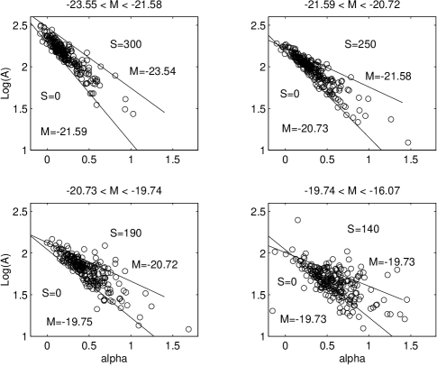
Figure 13: Surface-brightness boundaries shown for each magnitude-limited quartile

This is shown in the following manner: for each of the quartiles, which is magnitude-limited in its own specific range $(M_{min}<M<M_{max})$, we determine the surface-brightness limits, $(0<S<S_{max})$, which contain 95% of the sample (to eliminate the effects of long tails). Then, using the third-order model, $\log A=F(\alpha,\,M,\,S)$, we find that the distribution of points in each of the quartiles is closely bounded by the lines

$$\log A = F(\alpha,\,M_{max},0),$$

$$\log A = F(\alpha,\,M_{min},S_{max}),$$

in the $(\alpha,\,\log A)$ plane for each of the magnitude-limited quartiles. The results are shown in Figure 13, and the plots in the three brightest quartiles show very clearly that the lower boundaries of points in these quartiles coincide very closely with the $(S=0,\,M=M_{max})$ boundary in the plane, whilst the diffuse upper boundaries of points coincide very closely with the $(S=S_{max},\,M=M_{min})$ boundary in the plane.

The only partial exception to this rule is the plot in the dimmest magnitude-limited quartile. Here, the upper (very diffuse) boundary of points still coincides with the $(S=S_{max},\,M=M_{min})$ boundary; however, it was found that the $(S=0,\,M=M_{max})$ boundary is not even close to the lower boundary of points in the plot but, instead, we find that the lower-boundary of points follows closely the $(S=0,\,M=M_{min})$ boundary. The important point is that the lower boundary of points is still a $S=0$ boundary. The obvious explanation for this discrepancy is that objects of very low surface brightness and very high magnitude are observationally excluded by selection effects, and therefore do not exist in the dimmest quartile sample whilst, simultaneously, the same selection effects will also ensure that the low surface-brightness objects in the dimmest quartile will tend to be the low magnitude objects.

To summarize, the sharply delineated lower boundaries in the magnitude-limited quartiles of Figures 9 or 13 define a physical $S=0$ cut-off boundary, whilst the increasingly diffuse upper boundaries probably arise as a function of the increasing observational uncertainties associated with increasing magnitudes.

9 A Comparative Test Of The First, Second And Third-Order Models

The three models share the basic structure

$${V\over V_{0}}=\left({R\over R_{0}}\right)^{\alpha}$$ (11)

and are distinguished only by the models assumed for $(R_{0},\,V_{0})$. These three models are defined, respectively, according to:

The First-Order Model

$$\log R_{0} = 1.02,$$ (12)

$$\log V_{0} = 2.29;$$

The Second-Order Model

$$\log R_{0} = -2.27-0.14\,M,$$ (13)

$$\log V_{0} = -0.56-0.13\,M;$$

The Third-Order Model

$$\log R_{0} = -3.291-0.208\,M-0.00292\,S,$$ (14)

$$\log V_{0} = -0.584-0.133\,M-0.000243\,S.$$

As a final comparative test of these three models we note that, assuming each to be ‘correct’, then a linear regression of $\log(V/V_{0})$ data on $\log(R/R_{0})$ data should give rise to a statistically zero constant terms, indicating that the regression lines (tend to) pass through the origin. The distribution of these constant terms for each of the 900 rotation curves is given, for each of the three models, in Figure 14. To make the visual comparison easy, the three diagrams in the figure are each drawn to the same scale, and it is clear that the process of successively refining the model has the effect of tightening the distribution of $\log A$ about the zero-point. Specifically, the first-order model is comparatively very poor, whilst the third-order model is visually significantly better than the second-order model.

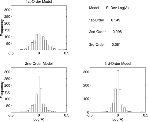
Figure 14: Comparative test of the three models

Table 8
One-parameter t-test for confidence
limits of Mean($\log A$)
Model	95% Interval	99.999% Interval
1st-Order	0.009,0.029	-0.003, 0.041
2nd-Order	-0.006,0.007	-0.014,0.015
3rd-Order	-0.003,0.007	-0.010,0.014

The results of a one-parameter t-test for limits on the position of the mean value of $\log A$ for each of the models are given in Table 8. Apart from showing that the $\log A$ distribution for the 1st-order model is slightly asymmetric with respect to the zero point, the table shows that the 2nd and 3rd-order models place very tight 95% and 99.999% confidence intervals on the mean of $\log A$ about the zero point. Thus, for all practical purposes, the regression constant computed over the 900 rotation curves is statistically zero in both the second and third-order models, so that these models receive the strongest possible support from the data.

10 Equivalence Classes Of Rotation Curves

As already discussed in detail in §6, the first-order model, equation (11) with (12), effectively defines the set of all rotation curves in the sample as a single class within which all the rotation curves pass through the single point $(\log R_{0},\,\log V_{0})$ in the $(\log R,\,\log V)$ plane.

By contrast, the second-order model, equation (11) with (13), replaces the single point, $(\log R_{0},\,\log V_{0})$, of the first-order model by a class of such points parametrized by $M$. All rotation curves in the class specified by $M$ then pass through the single point, $(\log R_{0},\,\log V_{0})$, defined by (13).

The third-order model, equation (11) with (14), is a refinement of the second-order model in which the class to which any given rotation curve belongs is defined by specifying $M$ and $S$, the surface brightness. All rotation curves in the class specified by $(M,\,S)$ then pass through the single point, $(\log R_{0},\,\log V_{0})$, defined by (14).

If we make the (reasonable) assumption that all of the systematic variation in the pivotal diagram, Figure 4, has been accounted for by the 90% third-order model then we can realistically assume that, although the functional form of the model is probably an approximation to some ideal, there are no further physical parameters involved in the specification of $(\log R_{0},\,\log V_{0})$. It will then follow that the rotation curves of all galaxies of having the same absolute magnitude and surfaces brightness will pass through a single point, $(\log R_{0},\,\log V_{0})$, in the $(\log R,\,\log V)$ plane. Consequently, all such rotation curves will be equivalent to within a rotation through the point, and can therefore be considered to define an equivalence class of rotation curves.

11 The Universal Rotation Curve

Using the third-order model, it is shown that the universal rotation curve for spiral galaxies can reasonably be assumed to have the general structure

$${V\over V_{0}} = \left({R\over R_{0}}\right)^{\alpha}$$ (15)

$$\log R_{0} = -3.291-0.208\,M-0.00292\,S,$$

$$\log V_{0} = -0.584-0.133\,M-0.000243\,S,$$

$$\alpha = g(d_{m},\,b_{m},\,h_{m})$$

where $g(d_{m},\,b_{m},\,h_{m})$ is some undetermined function for which the most significant parameters are probably the disc-mass, bulge-mass and halo-mass respectively of the spiral galaxy concerned.

11.1 The General Situation

Reference to (11) with (12), (13) and (14) shows that, once a model for $\alpha$ in terms of the physical properties of spiral galaxies is obtained, then (11) with any one of (12), (13) or (14) can be considered to represent a universal rotation curve. In the following, we consider the problem within the context of the third-order model.

As we have already noted, the issue depends entirely upon the function $\alpha$, and what galaxy parameters it is a function of.

Table 9
$\alpha=b_{0}+b_{1}\,M$
Predictor	Coeff	Std Dev	t-ratio	p
Const.	2.560	0.112	23	0.00
$M$	0.105	0.005	19	0.00
$R^{2}$  =  29.2%

A least-square linear modelling of $\alpha$ in terms of the available parameters, $M$ and $S$, gave the best model as $\alpha=-0.583+0.105\,M$, with no evidence of any significant dependency on $S$. The details of the best model are given in Table 9 which shows the dependency of $\alpha$ on $M$ to be extremely significant, but which also shows that the model accounts for only 29% of the total variation in the $(\alpha,\,M)$ plot (equivalent to a regression correlation of approximately 0.55). To test the possibility that the scatter in this latter plot was, perhaps, due to noisy data, we tried modelling on the brightest 25% and 50% of the data, but found no evidence at all to support this possibility. The only reasonable conclusion was that the unaccounted-for 71% variation in the $(\alpha,\,M)$ plot arises through the effects of unaccounted-for additional physical parameters.

The major unincluded determinants of disc dynamics are the relative amounts of disc-mass, halo-mass and bulge-mass. Consequently, defining $d_{m}\equiv$ disc-mass, $b_{m}\equiv$ bulge-mass and $h_{m}\equiv$ halo-mass, and noting that $M$ is effectively a measure of the total visible mass, then we can reasonably assert that $\alpha\approx g(d_{m},\,b_{m},\,h_{m})$.

11.2 A Simple Approximation

Finally, it is interesting to note how the foregoing analysis allows the construction of a very simply universal rotation curve, based on absolute magnitude alone. This is given by (11) and (13) together with the model for $\alpha$ described in Table 9 so that, specifically:

$${V\over V_{0}} = \left({R\over R_{0}}\right)^{\alpha}$$

$$\log R_{0} = -2.27-0.14\,M,$$ (16)

$$\log V_{0} = -0.56-0.13\,M,$$

$$\alpha = 2.560+0.105\,M,$$

which can be considered as a formal refinement of the information contained in Figure 8. This latter approximation confirms the conclusions of PS 1996 which are that the universal rotation curve is substantially determined by absolute magnitude alone, especially for the brightest galaxies.

12 Theory-Independent Dark-Matter Models

PSS, used essentially the same data set as that analysed here to show that whilst, at high luminosities, there is only a slight discrepancy between observed rotation curves and those predicted on the basis of the observed luminous matter distributions, the discrepancy is far more serious at low luminosities. This conclusion is already strongly supported by the simple model given at (16) which shows how the power-law exponent, $\alpha$, increases strongly with absolute magnitude. Since, (relatively) large values of $\alpha$ correspond directly to the most steeply rising rotation curves, and since it is precisely these kinds of rotation curves that require the largest amounts of dark matter for their explanation, according to the virial theorem, then the findings of the present analysis are in direct accord with those of PSS.

In this way, PSS have already used the data to show that the dark-matter component of spiral galaxies does not seem to have the form of an unconstrained and independent structure added onto the visible structure of spiral galaxies, but appears to make its presence felt in some kind of systematic way which is strongly inversely correlated with the visible component of the galaxy structure. This effect, together with the detailed considerations of the foregoing sections, allows the construction of dark-matter models which are independent of any particular dynamical theory and therefore, as a side effect, provide strong tests of such theories.

Specifically, referring to the final form of the universal rotation curve, given at (15), we see how dark-matter can only make its presence felt through the exponent, $\alpha$. Given that reasonable light-based estimates can be made of disc-mass ($d_{m}$) and bulge-mass ($b_{m}$) for spiral galaxies, then it is (in principle) a simple process to form empirical models of $\alpha$ directly in terms $d_{m}$ and $b_{m}$. Once such models are formed for a reasonably sized data-base of spiral galaxies, then it becomes a straightforward process to investigate the structure of any systematic deviations of predictions based on the model $\alpha\approx g(d_{m},\,b_{m})$ from the $\alpha$-values calculated directly from the rotation curves. The presence of any such systematic deviations can then reasonably be considered due to the presence of a dark-matter halo, so that, subsequently, estimates for the amount of dark-matter present for any given galaxy can be given in terms of the directly measurable properties of the galaxy concerned.

13 Conclusions

By demonstrating how completely the power-law model for rotation curves resolves rotation curve data, magnitude data and surface brightness data over a large data-base, this paper:

• substantially refines the well-known correlations that exist between the rotational kinematics of spiral galaxies and various of their non-kinematic properties, such as absolute magnitude;

• shows how the power-law rotation curve is, almost certainly, exact for idealized discs (that is, for discs without the irregularities inevitably present in real optical discs).

Additionally, at its lowest approximation, the analysis confirms the conclusion of PSS (1996) that the rotation curve of any given galaxy is largely determined by the absolute luminosity of the galaxy concerned, and supports their conclusion that absolute luminosity is inversely correlated with dark mass. Such an inverse correlation obviously provides a means of dark-matter modelling, but the detailed nature of the present analysis allows a further step in providing a means for the generation of statistical dark-matter models which are independent of any particular dynamical theory. Apart from the objective desirability of such models, they have an obvious potential in distinguishing between competing dynamical theories.

Furthermore, in showing that optical discs contain no signature of the transition from disc-dominated dynamics to halo-dominated dynamics, and in showing the existence of a strong correlation between $R_{min}$ and $R_{opt}$, the work provides very strong support for the conclusion of PS (1986) that the disc-mass distribution and the halo-mass distribution are very strongly correlated, and suggests that the bulge-mass distribution should also be factored into this correlation.

Appendix A The Constancy of ${\bar{V}}$

PS (1986) showed that the parameter

$${\bar{V}}\equiv\left(\Omega-{K\over 2}\right)R,$$

where $\Omega$ is angular velocity, and $K$, the epicyclic frequency, is defined by

$$K^{2}={1\over R^{3}}{d\over dR}\left(V^{2}R^{3}\right),$$

is almost constant over the larger part of any given optical disc for a sample of 42 spiral galaxies, and they deduce from this constancy that rotation curves contain no signature indicating transition from disc-dominated dynamics to halo-dominated dynamics. In the present case, the same conclusion can be drawn from the fact that the kinematics over the whole optical disc are amenable to description by a single power-law prescription. Such a power-law also provides an extra insight into the constancy of the ${\hat{V}}$ parameter:

Using the general power-law prescription $V=AR^{\alpha}$ in the above we find, after some algebra,

$${d{\hat{V}}\over dR}=A\,R^{\alpha-0.5}\left({\alpha\over\sqrt{R}}-{1\over 2}\left(\alpha+{1\over 2}\right)\sqrt{2\,\alpha+3}\right).$$

From this, we see that, whenever whenever a rotation curve is such that $\alpha<-0.5$, then the corresponding $d{\hat{V}}/dR$ rapidly becomes small for increasing $R$ - and this corresponds to a nearly constant ${\hat{V}}$. Reference to Figure 8 shows that this conditions holds for all galaxies brighter than $M\approx-20$ and, of the PS (1986) sample of 42 galaxies, 37 are brighter than $M\approx-20$ so that $\alpha<-0.5$ generally, indicating very flat ${\hat{V}}$ functions, as actually shown by PS.

Appendix B Data Reduction

A basic assumption is that optical rotation curves can be described in terms of a simple power law, and the validity of this assumption as, at the very least, a good approximation to the reality over the approximate range $(1,20)kpc$ has been demonstrated in §5.

However, spiral galaxies can be considered to consist of a spherical bulge surrounded by a flat disk, and we can be reasonably certain that the bulge and the disk represent distinct dynamical regimes. In practice therefore, the structure of the inner parts of rotation curves will be determined one dynamical regime, whilst the structure of the outer parts of the rotation curves will be determined by another. Since it is not reasonable to suppose that a single simple power law can bridge the two dynamical regimes, there is a need to find a way of eliminating the effect of the bulge dynamics from the rotation curve data. In order to ensure that no subjective bias is imposed on the data during such a data reduction process, the process adopted must be automatically applicable according to strictly predefined rules. The adopted procedure is described below.

The original analysis was done using the commercial statistics package, Minitab; when regressions are performed in Minitab, it automatically flags observations which have an unusual predictor or if they have an unusual response. In both cases ‘unusual’ is defined by internal parameters of the software. It was decided, in advance of any data processing, that when a Minitab regression flagged the innermost observation on any given rotation curve (that is, the one most likely affected by the central bulge) as ‘unusual’ then that observation would be deleted from the analysis, and the regression repeated. If, on the repeated regression, the new innermost observation was flagged as unusual, then it too would be deleted from the analysis. This process was repeated until the innermost observation remained unflagged after the regression process.

There are 900 rotation curves with a total of 19183 observations recorded with a non-zero radial coordinate (those with a zero radial coordinate were necessarily deleted because data was transformed into logarithmic form). Of these 19183 observations, the ‘innermost deletion’ strategy led to the exclusion of 2264 observations, which is $11.8\%$ of the sample. This was considered to be an acceptable attrition rate.

Appendix C Determination of Fixed Points, $(\log R_{0},\,\log V_{0})$

In §4 and §5 it was determined that the form of Figure 4 implied the first-order hypothesis that all rotation curves in the sample passed through a fixed point, $(\log R_{0},\log V_{0})$, in the $(\log R,\,\log V)$ plane. The problem is to determine the position of the fixed point $(\log R_{0},\,\log V_{0})$. In the following, we describe how this can be done using a minimization procedure.

The hypothesis implies that all 900 rotation curves in the sample should be equivalent to within a rotation about $(\log R_{0},\,\log V_{0})$; in this case it should be possible to superimpose all such rotations curves upon each other by means of a simple appropriate rotation. However, the very noisy nature of rotation curve data means that, at best, such a process of superimposition can only be defined in some averaged statistical way.

In practice, what is done can be characterized as follows:

• Define an initial guess for the fixed point $(\log R_{0},\,\log V_{0})$; this is done by the simple expedient of identifying the peaks of the rotation-curve intersection frequency distributions show in Figures 5 & 6, and they are found to be $\log R\approx 1.02$ and $\log V\approx 2.24$.

• Define a standard reference curve passing through the estimated fixed point; typically, this is done by making the arbitrary choice $\log A=1.5$ and then using (4) to determine $\alpha$.

• Rotate the data corresponding to each individual rotation curve about this estimated $(\log R_{0},\,\log V_{0})$ until it coincides in a least-square sense with the standard reference curve.

• Keep a cumulative sum of all the least-square residuals arising from the foregoing rotation operations performed on the individual rotation curves.

• Minimize this cumulative sum of least-square residuals with respect to variations in the estimated position of the fixed point, $(\log R_{0},\,\log V_{0})$.

Note that the minimization processes referred to above are minimizing functions defined on noisy data. It is routinely recommended that such problems are solved using the Simplex method, which is extremely robust - although slow. The original implementation of the method is given by Nelder & Mead (1965).

References

- [1] Burstein, D., Bender, R., Faber, S.M., Nolthenius, R., 1997 Global Relationships Among The Physical Properties Of Stellar Systems AJ 114 1365-1392.
- [2] Nelder, J.A., Mead, R., 1965 A Simplex Method For Function Minimization. Comp. J. 7 308-313
- [3] Mathewson, D.S., Ford, V.L., Buchhorn, M. 1992 A Southern Sky Survey of the Peculiar Velocities of 1355 Spiral Galaxies Astrophys J. Supp. 81 413-659.
- [4] Persic, M, Salucci, P., 1986 The Information on Large-Scale Properties of Spiral Galaxies Stored in Their Kinematics MNRAS 223 303-315.
- [5] Persic, M., Salucci, P., 1995 Rotation Curves of 967 Spiral Galaxies Astrophys. J. Supp. 99 501-541, astro-ph/9502091
- [6] Persic, M., Salucci, P., Stel, F., 1996 The Universal Rotation Curve of Spiral Galaxies 1. The Dark-Matter Connection MNRAS 281 27-47.
- [7] Rubin, V.C., Burstein, D., Ford, W.K., Thonnard, N., Rotation Velocities of 16 Sa Galaxies and a Comparison of Sa, Sb and Sc Rotation Properties Astrophys. J. 1985, 289, 81-96
- [8] Rubin, V.C., Ford, W.K., Thonnard, N. 1980 Rotational Properties of 21 Sc Galaxies With A Large Range Of Luminosities And Radii From NGC 4605 (R=4kpc) To UGC 2885 (R=122kpc) Astrophys. J. 238 471-487.