EXTREMELY METAL-POOR STARS. VIII. HIGH-RESOLUTION, HIGH-SIGNAL-TO-NOISE ANALYSIS OF FIVE STARS WITH [Fe/H] $\lesssim$ –3.5

Abstract

High-resolution, high-signal-to-noise ($\langle$S/N$\rangle$ = 85) spectra have been obtained for five stars – CD–24^o17504, CD–38^o245, CS 22172–002, CS 22885–096, and CS 22949–037 – having [Fe/H] $\lesssim$ –3.5 according to previous lower S/N material. LTE model-atmosphere techniques are used to determine [Fe/H] and relative abundances, or their limits, for some 18 elements, and to constrain more tightly the early enrichment history of the Galaxy than is possible based on previous analyses.

We compare our results with high-quality higher-abundance literature data for other metal-poor stars and with the canonical Galactic chemical enrichment results of Timmes et al. (1995) and obtain the following basic results: (1) Large supersolar values of [C/Fe] and [N/Fe], not predicted by the canonical models, exist at lowest abundance. For C at least, the result is difficult to attribute to internal mixing effects; (2) We confirm that there is no upward trend in [$\alpha$/Fe] as a function of [Fe/H], in contradistinction to some reports of the behavior of [O/Fe]; (3) The abundances of aluminum, after correction for non-LTE effects, are in fair accord with theoretical prediction; (4) We confirm earlier results concerning the Fe-peak elements that [Cr/Fe] and [Mn/Fe] decrease at lowest abundance, while [Co/Fe] increases – behaviors that had not been predicted. We find, however, that [Ni/Fe] does not vary with [Fe/H], and at [Fe/H] $\sim$ –3.7, [Ni/Fe] = +0.08 $\pm$ 0.06. This result appears to be inconsistent with the supernova models of Nakamura et al. (1999) that seek to understand the observed behavior of the Fe-peak elements by varying the position of the model mass cut relative to the Si-burning regions. (5) The heavy neutron-capture elements Sr and Ba exhibit a large scatter, with the effect being larger for Sr than Ba. The disparate behavior of these two elements has been attributed to the existence of (at least) two different mechanisms for their production; (6) For the remarkable object CS 22949–037, we confirm the result of McWilliam et al. (1995b) that [C/Fe], [Mg/Fe], and [Si/Fe] are supersolar by $\sim$ 1.0 dex. Further, we find [N/Fe] = 2.7 $\pm$ 0.4. None of these results is understandable within the framework of standard models. We discuss them in terms of partial ejection of supernova mantles (Woosley & Weaver 1995) and massive (200–500 M_⊙) zero-heavy-element hypernovae (e.g. Woosley & Weaver 1982). The latter model actually predicted overproduction of N and underproduction of Fe-peak elements; and (7) We use robust techniques to determine abundance trends as a function of [Fe/H]. In most cases one sees an apparent upturn in the dispersion of relative abundance [X/Fe] for [Fe/H] $<$ –2.5. It remains unclear whether this is a real effect, or one driven by observational error. The question needs to be resolved with a much larger and homogeneous data set, both to improve the quality of the data and to understand the role of unusual stars such as CS 22949–037.

Suggested running title:     FIVE STARS WITH [Fe/H] $\lesssim$ –3.5

1 INTRODUCTION

Two decades ago no stars were known with chemical abundance [Fe/H] $<$ –3.0 (heavy elements less that 1/1000 solar) (Bond 1981). Today, as the result of systematic searches, in particular the HK survey of Beers, Preston, & Shectman (1985, 1992), we know of $\sim$ 100 such objects (Beers et al. 1998; Norris 1999). The most metal-poor stars in these surveys have [Fe/H] = –4.0 (McWilliam et al. 1995b; Ryan, Norris, & Beers 1996).

The chemical abundances of objects with [Fe/H] $<$ –3.0 contain clues to conditions at the earliest times. As outlined in the previous paper of this series (Norris, Beers, & Ryan 2000) they constrain Big Bang Nucleosynthesis (Ryan, Norris, & Beers 1999; Ryan et al. 2000), the nature of the first supernovae (McWilliam et al. 1995b; Ryan et al. 1996; Nakamura et al. 1999), the manner in which the ejecta from the first generations were incorporated into subsequent ones (Ryan et al. 1996; Shigeyama & Tsujimoto 1998; Tsujimoto & Shigeyama 1998; Ikuta & Arimoto 1999; Tsujimoto, Shigeyama & Yoshii 1999), and (in special cases) the age of the Galaxy (Cowan et al. 1999; Cayrel et al. 2001). Having formed at an epoch corresponding to redshifts $\gtrsim$  4–5, they nicely complement and constrain abundance results from the more complicated and less well-understood Lyman–$\alpha$ clouds and Damped Lyman–$\alpha$ systems currently studied at redshifts z $<$ 4.5 (Songaila & Cowie 1996; Pettini et al. 1997; Prochaska & Wolfe 1999; Dessauges-Zavadsky 2001). The field is understandably an active one.

At lowest abundance, the absorption lines upon which analysis is based weaken dramatically, and one needs to accurately measure features having equivalent widths $\lesssim$ 10–15 mÅ. For digital spectra, the error associated with the integration over an absorption line can be written $\sigma_{\rm W}\simeq$ ($\lambda\sqrt{\rm{n_{pix}}}$)/(R x [S/N]), where R is the resolving power, S/N is signal-to-noise/pixel, n_pix is the number of pixels over which the integration is performed, and the assumption is made that the width of the instrumental profile is a fixed number of pixels. If one assumes further that n_pix is constant for different observers, one can define a figure of merit F = (R x [S/N])/$\lambda$, which should be maximized for best results. Table 1 compares F for recent spectroscopic investigations of stars having [Fe/H] $<$–3.0. One sees that F varies in the range 85–500 Å^-1. This translates, roughly, to 3$\sigma$ errors in line strength measurement between 35 and 6 mÅ, respectively. To make definitive progress in this field one thus needs observational material having F $\gtrsim$ 500. Perhaps the most comprehensive studies of the past decade have been those of McWilliam et al. (1995b) and Ryan et al. (1996), but as may be seen from Table 1 the quality of their data was somewhat limited, driven by a desire to survey the properties of newly-discovered objects having [Fe/H] $<$ –3.0. Their sample sizes, with only 14 and 10 stars, respectively, having [Fe/H] $<$ –3.0, have also limited progress. One might expect that the high-dispersion spectrographs currently being deployed on 8–10 m class telescopes will permit the study of larger samples at higher precision.

In an attempt to provide more accurate abundances at lowest abundance we decided to obtain high-resolution, high signal-to-noise data for six stars which, according to earlier analysis, have [Fe/H] $<$ –3.5. These objects were chosen with absolutely no bias concerning their relative abundances, [X/Fe], and within the caveat of small numbers provide a representative sample of the most metal-poor stars. Our aim was to obtain accurate relative abundances with a view to more closely constraining conditions at the earliest times. We were particularly interested to establish, where possible, the lowest abundance anchors to observed relative abundance trends. We also wished to investigate the question of abundance spreads below [Fe/H] = –2.5: in the case of [Sr/Fe], for example, there exists a large and significant spread, but for other elements the situation is presently not clear.

The results for CS 22876–032, the most metal-poor dwarf in the sample (also a double-lined spectroscopic binary), have already been reported (Norris et al. 2000). Here we present high-resolution (R = 42000), high-signal-to-noise spectroscopy (S/N $\sim$ 40–100 per 0.04 Å pixel) and elemental abundance analyses for the remaining five stars. The objects are CD–24^o17504, CD–38^o245, CS 22172–002, CS 22885–096, and CS 22949–037. The reader should see Table 6 of Ryan et al. (1996) for details of previous analyses. The mean S/N for the new data set is $\sim$ 85, yielding F = 830 (as presented in Table 1).

The data and their analysis are reported in §2 and §3, respectively. In §4 we discuss the implications of our findings. The results strengthen earlier conclusions that existing models of supernovae explosions and Galactic chemical enrichment fail to fully reproduce observed enrichment at the earliest times. There is also support for the view that hypernovae (M $\gtrsim$ 100 M_⊙ pair-instability supernovae) may have played a role in that enrichment.

2 OBSERVATIONAL MATERIAL

High-resolution spectra were obtained with the University College London coudé échelle spectrograph on the Anglo-Australian Telescope during August 1996, 1997, and 1998, and in September 2000. The instrumental setup and data reduction techniques were similar to those described by Norris, Ryan, & Beers (1996) and Norris et al. (2000), and will not be discussed here, except to repeat that the material covers the wavelength range 3700–4700 Å and was obtained with resolving power 42000. The numbers of detected photons in the spectra were 10500, 9800, 2500, 8500, and 3300 per 0.04 Å pixel at 4300 Å for CD–24^o17504, CD–38^o245, CS 22172–002, CS 22885–096, and CS 22949–037, respectively. (It is perhaps worth noting for completeness that the counts diminish towards shorter wavelengths, and have decreased to roughly 65% of these values at 3900 Å.) In the case of CS 22172–002 the data were co-added to our earlier material (Norris et al. 1996) to yield S/N $\sim$ 70 per 0.04 Å pixel.

Examples of the spectra are presented in Figure 1 (which covers the residual intensity range 0.5–1.0) together with those of the well-studied halo subgiant HD 140283 ([Fe/H] = –2.5) and giant HD 122563 ([Fe/H] = –2.7) (from Norris et al. 1996), in the region of the G band of the CH molecule. The G band is clearly seen in the standard stars, and is surprisingly strong in CS 22949–037, as was first noted by McWilliam et al. (1995b). We shall return to this point in §4.

2.1 Line strength measurements

Equivalent widths were measured for the lines of 15 ionization species in 13 elements for most of the program stars, together with upper limits for those of three other important elements using techniques described in Norris et al. (1996, 2000). The results are presented in Table 2. The upper limits to line strengths listed in the table reflect estimates of the detectability of lines formed during the interactive line measurement process. Post facto one finds that they are a little larger than formal $\sim$ 3$\sigma$ measurement errors. (For our spectra $\sigma_{\rm W}$ = 120/(S/N) mÅ, leading to 3$\sigma$ errors of 4, 4, 5, 4, and 6 mÅ for CD–24^o17504, CD–38^o245, CS 22172–002, CS 22885–096, and CS 22949–037, respectively). The corresponding upper limits in Table 2 are 4, 5, 8, 5, and 10 mÅ.

Comparisons between the line strengths of the present work and previous investigations are presented in Figure 2, together with the figure of merit F, defined above. The diagram is not meant to be a comparison of the best data with the best data, but rather to demonstrate the role F plays in describing the quality of the material. The agreement is quite satisfactory, with the scatter in the diagrams being in qualitative agreement with the values of F. Quantitatively, the RMS scatter about linear regressions between the data of different observers were 4, 10, 11, and 17 mÅ for CD–24^o17504, CD–38^o245, CS 22885–096, and CS 22949–037, respectively. One may compare these with values of $\sigma_{\rm W}$ determined from photon statistics. We estimate that the corresponding quadratically added 1$\sigma$ measurement errors are, roughly, 2, 5, 6, and 8 mÅ. While the sense of the agreement is correct, the comparison suggests that the latter estimates may be somewhat optimistic.

2.2 Radial Velocities

Radial velocities were determined with techniques described in earlier papers of this series (Norris et al. 1996, 1997a, 2000) and Aoki et al. (2000). The results are presented in Table 3, together with independent values from the literature. We note that column (4) contains the internal standard error of the present measurements. Norris et al. (1996) claim an “upper limit to the external standard deviation of a single observation of 1 km s^-1,” which should also pertain to the present observations. Comparison of our velocities with the independent estimates in Table 3 show no evidence for variability above the 1 km s^-1 level in any of the objects for which multiple observations exist.

3 CHEMICAL ABUNDANCES

3.1 Abundances

Full details of the techniques of abundance determination have been presented in Ryan et al. (1996) and Norris et al. (1997a, 2000) and will not be repeated here, except to draw the reader’s attention to the following points.

We assume that line formation takes place under conditions of Local Thermodynamic Equilibrium (LTE) and adopt the model atmospheres of Bell et al. (1976) and Bell (1983, private communication). All calculations are performed with codes that derive from the original ATLAS formalism (Kurucz 1970; Cottrell & Norris 1978). Measured BVRI colors and estimates of interstellar reddening, presented in Table 4, form the basis of effective temperature determination via the calibrations of Bell and Oke (1986), Buser & Kurucz (1992), and Bell & Gustafsson (1978, 1989). Surface gravity is determined, in the first instance, by assuming that the star in question lies on a canonical pre-helium-flash evolutionary track in the color-magnitude diagram, and refined by the requirement that derived abundances of Fe I and Fe II are identical. Finally, microturbulent velocities, $\xi$, are determined by requiring that abundances derived for individual lines should exhibit no dependence on equivalent width.

The atmospheric parameters for the program stars are presented in columns (7)–(10) of Table 4, where the column headings should be self explanatory. Column (9) is our final [Fe/H] and the value adopted for the model atmosphere calculations. Relative abundances (together with [Fe/H]), their errors, and the number of lines used in the analysis are presented in Table 5. We note that the Si abundances in the giants are based not only on the equivalent width of the single unblended 3905.5 Å line (Table 2) but also on spectrum synthesis of the 4102.9 Å line, which lies in the wing of H$\delta$.

For carbon and nitrogen the abundances are based on spectrum synthesis of the $\lambda$4323 Å feature of CH and the $\lambda$3883 Å bandhead of CN, respectively, as described in Norris et al. (1997a). (In the absence of information on the abundance of oxygen we assume [O/Fe] = 0.6, and note that for the program stars the results are insensitive to variations of $\Delta$[O/Fe] = $\pm$0.4.) A comparison of observed and synthetic spectra is presented in Figure 3 for four of the program stars, as well as for the more metal-rich Population II stars HD 122563 and HD 140283. Carbon is detected in three of the five program stars, and for CS 22885–096 and CS 22949–037 the present results confirm earlier values reported by McWilliam et al. (1995b), albeit with somewhat higher accuracy.

Nitrogen is detected in only CS 22949–037. The claimed overabundance, [N/Fe] = 2.7 $\pm$ 0.4, is both astounding and, at first sight, almost unbelievable. In an effort to convince ourselves that the result was not an artifact of the measurement procedure (in particular faulty cosmic ray removal) we re-examined the observational material in some detail. In the initial analysis, cosmic rays had been removed using the BCLEAN and CLEAN utilities of the reduction package FIGARO. In the re-analysis they were removed in two different ways. On each of the four nights during which the data were obtained, median and 2$\sigma$ clipped average images were obtained and then added to form the final spectra. In both cases the essential result remained unchanged. Further, the CN bandhead is seen in the data subsets on individual nights. As a final check, the reduction was repeated by a different author using the IRAF reduction package. The same result was obtained.

After the present analysis was completed, a service observation of CS 22949–037 was obtained with the William Herschel Telescope/Utrecht échelle spectrograph combination. It provides confirmation of the existence of an absorption feature at 3883 Å from an independent dataset, albeit at much lower S/N = 14.

3.2 Random errors

The abundance errors for atomic species deserve comment. Random errors arise from those associated with line-strength measurements and with the determination of atmospheric parameters (uncertainties in colors, etc.), while systematic ones result from the (color, effective temperature)-calibrations and the analysis procedure itself (assumption of LTE, choice of model atmosphere, etc.). The errors listed in Table 5 address only random errors: they represent the quadratic addition of the standard error in abundance (the error in the mean abundance) derived from individual lines and errors resulting from atmospheric parameter uncertainties $\Delta$T_eff = 100 K, $\Delta$log $g$ = 0.3, and $\Delta\xi$ = 0.25 km s^-1, which we believe to be appropriate for the present investigation.

3.3 Systematic errors

Systematic errors are more difficult to assess. We have discussed elsewhere (Ryan et al. 1999) differences that arise between alternative plausible choices of effective temperature scales. For example, Alonso, Arribas, & Martinez-Roger (1996) have determined temperatures using the Infrared Flux Method (IRFM) that are generally higher than those from BVRI colors and model atmospheres. In order to quantify the effect, we assessed the impact on our analysis had we adopted IRFM-related temperatures. Due to the $\sim$1000 K difference between CD–24^o17504 and the giants, we address these two groupings separately.

The turnoff/subgiant star CD–24^o17504 has an IRFM T${}_{\rm eff}=6375$ K (Alonso, private communication to Primas et al. 2000), some 300 K hotter than adopted here. To assess the effect of using the IRFM scale, we repeated our analysis using that higher temperature. The resulting atmospheric parameters were T_eff/log $g$/[Fe/H]/$\xi$ = 6375/4.2/$-$3.15/1.4, indicating a surface gravity higher by 0.6 dex, and [Fe/H] higher by 0.22 dex. (Inferred Fe I abundances in Population II turnoff stars increase by $\sim~{}0.07$–0.08 dex per 100 K.) Columns (2) and (3) of Table 6 present abundances determined in the present work and those obtained by using IRFM based atmospheric parameters, respectively, while column (4) contains relative abundance differences in the form $\Delta$[X/Fe] = [X/Fe]_IRFM $-$ [X/Fe]${}_{\rm This~{}work}$. All differences are relatively small: typical (RMS) differences are 0.06 dex for neutral lines and 0.12 dex for ionized lines (excluding Fe II, the agreement of which was forced in determining log $g$). These are comparable to the 1$\sigma$ random errors already listed in Table 5, whose RMS values for neutral and ionized lines are 0.10 and 0.14 dex, respectively, in this star.

For the four giants of the present study, IRFM temperatures are unavailable, but it is possible to transform the BVRI colors to the IRFM scale using the color-metallicity-temperature calibrations provided by Alonso, Arribas, & Martinez-Roger (1999). Using the Johnson-Cousins photometry from our Table 4, Cousins-to-Johnson transformations from Bessell (1979), and Johnson-to-IRFM calibration equations from Alonso et al. Table 2, we find the temperatures given in Table 7. The heading of each IRFM column includes the equation number of the calibration. It was necessary to extrapolate outside the stated range of validity of the Alonso et al. calibrations (see their Table 3) because of the dearth of calibrating stars with [Fe/H] $<$ $-3$; although such extrapolations can be misleading, IRFM temperatures are nevertheless being adopted by many other workers in this field, and a comparison of the two scales may be instructive. The entries based on $V-R$ and $R-I$ are flagged as uncertain because the calibrations show greater sensitivity to metallicity between [Fe/H] = –3 and [Fe/H] = –2 than they do between [Fe/H] = –2 and [Fe/H] = –1, which is unlikely to be correct; see Alonso et al. (1999) Table 6 and the discussion of this issue by Ryan et al. (1999), especially their Fig. 5. The final column of Table 7 gives for each star the difference between the mean of the IRFM-scale temperatures and the temperature we have adopted in Table 4. The differences are small in all cases except one, $\Delta$T_eff = 103 K for CS 22949–037, but even that difference is smaller than the formal 1$\sigma$ errors associated with the Johnson-to-IRFM calibrations of 96–167 K (see final row of Table 7, transcribed from Alonso et al. Table 2). The comparison suggests that even if we had adopted IRFM-scale temperatures for the giants, the changes would have been minor. Columns (5)–(7) of Table 6 show the abundance changes that result for CS 22949–037 if we adopt the higher temperature, which leads to atmospheric parameters T_eff/log $g$/[Fe/H]/$\xi$ = 5000/1.9/$-$3.72/2.0. The largest change in [X/Fe] is 0.07 dex, and for most species it is considerably smaller. (We note for completeness that adoption of the hotter model would lead to higher relative abundances of carbon and nitrogen by 0.05 dex.)

As discussed by Ryan et al. (1996, §3.2.1) the adoption of different model atmospheres will also lead to small systematic differences. They found $\Delta$[Fe/H] $\sim$ 0.10 and 0.15 for dwarfs and giants, respectively, between analyses using Kurucz (1993) models and those of Bell and coworkers used here. The origin of this effect was attributed to differences of order 200 K in the temperature in the line forming regions, arising from the higher convective energy transport of the Kurucz models.

During the analysis of the giants, a curious dependence of derived abundance on excitation potential $\chi$ was noticed for the neutral iron lines. (It is not clear whether other atomic species are affected; neutral iron has the largest number of lines, so any abnormal effects are clearer.) Fe I lines in the range $\chi$ = 1.4–3.3 eV show no dependence on $\chi$, but the lower excitation lines give an abundance higher by 0.2–0.3 dex at $\chi$ = 0. Note that no such trend is seen either for the dwarf, CD$-$24^∘17504, or in our analysis of the higher-metallicity halo giant HD 122563 ([Fe/H] = $-2.68$), for which we also have high-quality data (Ryan et al. 1996). Although the microturbulence $\xi$ can in principle affect $\chi$-residuals (since on average lower-excitation lines tend to give rise to stronger lines), tests showed that it was not possible by adjusting $\xi$ to remove the $\chi$ trend and simultaneously get a sensible [Fe/H] versus equivalent width relationship.

We considered the possibility that errors in the temperature gradients of our adopted one-dimensional models might be too shallow, i.e. the outer layers too hot compared with the result for three-dimensional models found by Asplund et al. (1999). Low-$\chi$ lines having (on average) higher line strength and hence forming (on average) further out would then be computed too weak and higher abundances would be derived. However, the exclusion of stronger lines had little effect on the pattern, and the fact that the dwarf was not affected, whereas Asplund et al’s analysis was for dwarfs, made us doubt this possibility.

McWilliam et al. (1995b) reported $\chi$ trends when they used Bell & Gustafsson (1978, 1989) T_eff scales, so they used those calculations only to trace the metallicity sensitivity, and tied the colors to a solar-metallicity calibration of McWilliam (1990). They derive temperatures approximately 100 K cooler. However, an arbitrary decrease of 100 K in the effective temperatures of our models changes only the overall slope of the $\chi$-trends (and to the degree expected from stellar atmosphere theory); it does not alter the distortion of low- versus high-excitation lines. We can only surmise that McWilliam et al. found a simpler trend.

We tried replacing the modified van der Waal’s damping values used by Ryan et al. 1996, §3.3) with those from Anstee & O’Mara (1995), Barklem & O’Mara (1997), and Barklem, O’Mara, & Ross (1998), but this had very little effect ($\leq 0.03$ dex) on the abundances and none at all on the $\chi$-trends. (Very metal-poor stars have few high-excitation-potential lines, so are much less affected by the $\chi$-dependent damping errors discussed by Ryan (1998).)

An alternative is that non-LTE effects are present, possibly consistent with the peculiarity showing up in the giants but not the dwarf. One possible effect of relying on an LTE analysis is that Fe II/Fe I ratios produce the wrong gravity (see below). We examined the Fe I/Fe II and Ti I/Ti II ratios to see what gravities would be inferred. The differences were random, and suggested an internal uncertainty $\Delta$ log g $\lesssim$ 0.3 dex, entirely consistent with the observational uncertainties in [Fe II/Fe I] of 0.07–0.13 dex. (A 0.10 dex error in the abundance ratio leads to a 0.33 dex error in the gravity.) Trying giants with gravities arbitrarily 0.8 dex higher improved the picture only slightly, leaving us unconvinced that this was the correct (or even a viable) solution.

The assumptions of LTE, one-dimensional models, and the treatment of convection in terms of the mixing-length approximation all have the potential to seriously compromise the results presented here. Non-LTE effects can be important, as demonstrated by Baumüller and Gehren (1997) for the resonance lines of Al I (see §4.1.4 below). For other elements, however, there exist conflicting results: for iron, e.g., Thévenin & Idiart (1999) and Gratton et al. (1999) reported quite different conclusions. The former found a large degree of over-ionization in metal-poor stars, which they attributed to the lower line opacity and hence higher (more important) UV radiative flux in low-metallicity atmospheres. They suggested two consequences: (1) spectroscopically-determined log $g$ values based on LTE analyses will be too low, by up to 0.4–0.6 dex for dwarfs at [Fe/H] $\sim-3$, and (2) abundances derived from the minority ionization state (Fe I) will be too low by $\sim$ 0.3 dex at [Fe/H] $\sim-$3. A comparison of trigonometric and spectroscopic log $g$ determinations by Allende Prieto et al. (1999) showed a similar metallicity dependence, but their analysis also emphasised that the magnitude of the correction varied considerably from one study to the next (e.g. their Figures 7 and 10), such that corrections derived in one study could not necessarily be applied to another. Gratton et al. (1999), in contradistinction to the other two works, found no strong effect in dwarf atmospheres.

It has also become clear that realistic three-dimensional modeling of metal-poor stars, and the consequent rigorous treatment of stellar convection, may significantly modify the abundances presented here. Preliminary results of Asplund et al. (1999) for stars having [Fe/H] $\sim$ $-2.5$ show that modifications to LTE 1D model abundances of order 0.2 dex may be necessary, though they also found (Asplund & Nordlund 2000) that for Li I at least, non-LTE 3D computations gave very similar abundances to LTE 1D calculations.

Clearly both non-LTE computations and 3D modeling are rapidly developing fields whose ultimate implications have yet to become clear. The reader should bear these caveats in mind when reading the following section.

4 DISCUSSION

4.1 Relative Abundances, [X/Fe], as a Function of [Fe/H]

The present results permit us to re-visit relative abundance trends as a function of [Fe/H], following Ryan et al. (1996) and Norris et al. (1997a). Figures 4–9 present [X/Fe] versus [Fe/H] based on the results in Table 5 and those from the literature.

4.1.1 Carbon & Nitrogen

Figure 4 presents [C/Fe] as a function of [Fe/H], where the results from Table 5 are supplemented by data from McWilliam et al. (1995b), Norris et al. (1997a), Ryan et al. (1991), and Tomkin et al. (1992, 1995). Stars with [C/Fe] $>$ +1.5 are not considered in the present discussion. (These include objects with very large over-abundances of s-process heavy elements (Norris et al. 1997a; Aoki et al. 2000; Hill et al. 2000) that are believed to have resulted from mass transfer across a binary system, together with the enigmatic CS 22957–027 ([Fe/H] = –3.4, [C/Fe] = +2., but “normal” heavy neutron-capture element abundance; Norris, Ryan, & Beers 1997b, Bonifacio et al. 1997). While the s-process enriched objects tell us about nucleosynthesis in intermediate mass stars, it remains to be seen what the relationship is between CS 22957–027 and the stars studied here.) Also shown in the figure is the standard stellar evolution, Galactic chemical enrichment (GCE) prediction of Timmes et al. (1995) (without modification of their computed Fe yield).

The data in the present paper strengthen the conclusion that there is a large spread in carbon at lowest abundance. At [Fe/H] $<$ –3.0, the range in [C/Fe] is of order 1 dex. It is important to note that this large spread is not an observational selection effect: none of the stars with [Fe/H] $<$ –3.0 in Figure 4 was chosen for study with any knowledge relating to its carbon abundance. (Rossi, Beers, & Sneden (1999) have discussed large numbers of metal-poor, C-rich stars, but for a C-enhanced selected sub-sample, drawn post facto from the HK medium-resolution follow-up spectroscopy campaign.) Part of the spread (for giants) may result from the internal mixing of CNO processed material into outer layers during giant-branch evolution as has been invoked to explain carbon depletions observed in the most metal-poor globular clusters (Kraft et al. 1982; Langer et al. 1986). Such an explanation is not inconsistent with the fact that CD–38^o245 (Fe/H] = –3.98, [C/Fe] $<$ 0.00) is nitrogen rich ([N/Fe] = 1.7, with a possible zero-point error of 0.6 dex, Bessell & Norris 1984). If such mixing has indeed occurred, any giant that now has [C/Fe] $>$ 0.0 could have originated with an even larger carbon abundance. The more important point here, however, is that whatever the role of mixing, real and large supersolar [C/Fe] values exist at lowest metallicity. Furthermore, as may be seen in Figure 4, such overabundances are not predicted by canonical GCE models, suggesting that simulations of the most metal-poor supernovae or mass-loss during late stages of massive-star evolution are incomplete. We shall return to this point in §4.2.

As noted in §3.1, the value of [N/Fe] = +2.7 for CS 22949–037 is surprisingly large. If, in the absence of any knowledge concerning the abundance of oxygen, one were to suppose that the overabundance of nitrogen arose from internal mixing of equilibrium CN-cycle processed material into the star’s outer layers as discussed above, one is led to an initial carbon abundance [C/Fe] = +2.1. The alternative is that both carbon and nitrogen were enormously enhanced in the ejecta of the object which enriched the material from which CS 22949–037 formed. We defer consideration of this possibility to §4.2, following discussion of the abundances of the other elements.

4.1.2 Heavier Elements

For elements heavier than carbon we use comparison material based on observations similar in quality to those in Table 2, by only accepting abundances derived from data having figure of merit F $>$ 300 (F is defined in §1). (This choice of the limit is of course arbitrary, since the accuracy of abundances will be a function of the number of lines and the strength of those lines for a given element. We seek here only to apply the coarsest of cuts to literature sources.) Where possible we have corrected the published values for differences between the literature solar abundances and those adopted here (Table 5, column (3)). The literature sources are Gilroy et al. (1988), Gratton (1989), Gratton et al. (1987, 1988, 1991, 1994), Ryan et al. (1991, 1996), Nissen & Schuster (1997), Carney et al. (1997), Stephens (1999), and Fulbright (2000). (We discuss in the Appendix a modification we have made to a critical literature $gf$ value for Co I.)

The comparisons are presented in Figures 5–9 . As in Ryan et al. (1996) the left panels of the figures permit one to examine the origin of the data. (Error bars are attached to stars from the present study, and to CS 22876–032 ([Fe/H] = –3.71, Norris et al. 2000; open circle), while results for objects having more than one analysis are connected. For Ti we plot the results for Ti II, which differ insignificantly from the average of Ti I and Ti II (weighted by the number of lines involved.)) The right panel presents the data anonymously, together with abundance trends determined with robust statistical tools. The thin lines represent loess regression lines described by Cleveland (1994), and determined as follows. First, average values of each abundance ratio were obtained if results were available from different authors. Next, we obtained three vectors – the central loess line (CLL), the lower loess line (LLL), and the upper loess line (ULL), as a function of the [Fe/H] values. The CLL is defined as the loess line obtained when all the data are considered, and provides our best estimate of the general trend of the elemental ratios at a given [Fe/H] – this line replaces the midmean trend line considered previously by Ryan et al. (1996). Next, residuals about the CLL were obtained, and separated into those above (positive residuals) and below (negative residuals) this line. The LLL is defined as the loess line for the negative residuals as a function of [Fe/H] – this replaces the lower semi-midmean considered by Ryan et al. (1996). The ULL is defined as the loess line for the positive residuals as a function of [Fe/H] – this replaces the upper semi-midmean considered by Ryan et al. (1996). If the data are scattered about the CLL according to a normal distribution, the LLL and ULL are estimates of the true quartiles. The loess summary lines have an advantage over the midmeans and semi-midmeans used by Ryan et al., in that one is not forced to arbitrarily bin the data in order to preserve resolution while suppressing noise. The loess lines remain sensitive to local variations without being unduly influenced by outliers. Furthermore, they are able to better handle the endpoints of the data sets. In each subpanel the CLL is flanked by the ULL and CLL. Also shown in the figures as thicker dashed lines are the GCE predictions of Timmes et al. (1995).

4.1.3 The $\alpha$-Elements: Mg, Si, Ca, and Ti.

The trends in Figure 5 collectively show that there is no strong change of [$\alpha$/Fe] with [Fe/H] in the range –4 to –1, consistent with previous investigations. This is in marked contrast with recent reports that [O/Fe] increases monotonically as [Fe/H] decreases, with d[O/Fe]/d[Fe/H] $\sim$ –0.33 in the range –3.0 $<$ [Fe/H] $<$ 0.0 (Israelian, Garcia López, & Rebolo 1998; Boesgaard et al. 1999). Elements lighter than calcium are chiefly produced during hydrostatic burning in stars, and the GCE models of Timmes et al. (1995) show little dependence of [O, $\alpha$/Fe] on [Fe/H] under the assumption that hydrostatically burned regions are expelled during the supernova phase. Insofar as theory requires a coupling between the behavior of O and $\alpha$-elements, the present results do not offer support for the claimed upward trend of [O/Fe] with decreasing [Fe/H]. That said, we refer the reader to Israelian et al. (2001) for the case that “there is a range of parameters in the calculations of nucleosynthesis yields from massive stars at low metallicities that can accommodate (an increase of [O/Fe] with decreasing [Fe/H])”. We note also, as emphasized to us by the referee, that decoupling between O and the $\alpha$-elements exist in some of the supernova models reported by Woosley & Weaver (1995).

Excluding CS 22949–037, the relative $\alpha$-element abundances of the stars studied here appear to be quite similar, except for Si, where a large spread is evident. Given that the Si values are not as well-determined as those for the other elements, we believe it would be premature to interpret the large scatter of this element as originating from other than error of measurement, and we shall thus not discuss the apparent Si spread further.

Concerning CS 22949–037, we confirm the result first reported by McWilliam et al. (1995b) that [$\alpha$/Fe] is larger in this star than in other extremely metal-poor stars. We also find that the size of the difference appears to decrease with increasing atomic number within the $\alpha$-element class: if we compare CS 22949–037 with (as a group) the other four stars studied here we obtain $\Delta$[Mg/H] = 0.77 $\pm$ 0.14, $\Delta$[Si/H] = 0.75 $\pm$ 0.31, $\Delta$[Ca/H] = 0.25 $\pm$ 0.21, and $\Delta$[Ti/H] = 0.07 $\pm$ 0.17. The corresponding values from the results of McWilliam et al. for CS 22949–037 relative to their mean sample values are 0.80 $\pm$ 0.16, 0.35 $\pm$ 0.33, 0.46 $\pm$ 0.15, and 0.22 $\pm$ 0.15, respectively. The agreement is excellent.

One may re-visit the discussion of McWilliam et al., who noted that these results are suggestive of only partial ejection of the stellar mantle during the supernovae explosion(s) that enriched the material from which CS 22949–037 formed. Woosley and Weaver (1995) report supernovae simulations with relatively low ejection velocities in which no Fe is ejected, but with expulsion of some of the lighter elements. Consider, in particular, their model Z35B for a zero heavy element, 35 M_⊙, intermediate-energy explosion in which they report production factors of 4.2, 7.2, 3.3. 0.09, 0.00, 0.00, and 0.00 for ¹²C, ¹⁶O, ²⁴Mg, ²⁸Si, ⁴⁰Ca, ⁴⁸Ti, and ⁵⁶Fe, respectively. The atomic-mass dependence of the yield of this model is broadly able to explain the trends seen in CS 22949–037, though the particular model quoted produces little Si. A slightly lower location, however, of the mass-cut presumably might rectify this mismatch, as ⁴⁰Ca and ⁵⁶Ni (the parent of ⁵⁶Fe) are formed deeper than much of the ²⁸Si and all of the ²⁴Mg. In principle it might be possible to eject larger amounts of Mg and Si while ejecting little Ca and iron-peak elements. (See likewise the models of Umeda, Nomoto, & Nakamura (2000).) We shall discuss this question further in §4.2.1.

Nucleosynthesis models currently neglect mixing of deeper material into the outer layers, although at least some observations of SN II (Fassia et al. 1998; Fassia & Meikle 1999) and their ejecta (Travaglio et al. 1999) seem to require it. Such mixing may provide an alternative means of producing partial iron-peak element enrichment of the ejected Mg–Si envelope.

4.1.4 Aluminum

The results for [Al/Fe] and [Al/Mg] are presented in Figure 6. They are based on only the Al I 3961.5 Å line, given the possible contamination of Al I 3944.0 Å by CH, as first suggested by Arpigny & Magain (1983), and the support for this claim by our finding that the line is broader than expected in C-enhanced stars (Ryan et al. 1996, §3.4.4).

For stars of the lowest metallicity, Al abundances are necessarily based on the resonance lines used here, since other lines of the species lie below the detection limit. This unfortunately leads to large systematic errors. Baumüller & Gehren (1997) have demonstrated that for dwarfs with [Fe/H] $\sim$ –3.0, LTE analysis of Al I 3961.5 Å leads to an error $\Delta$[Al/H] = –0.65. For [Fe/H] $>$ –2.0, in contrast, use of the Al I lines near 6697 Å leads to errors of only $\sim$ –0.15. It remains to be seen how large the non-LTE corrections are for giants. We note that for [Fe/H] $<$ –3.0 our analysis yields essentially the same behavior of [Al/Fe] for both giants and dwarfs.

We also comment on the distribution of the data in the ([Al/Fe], [Fe/H])- and ([Al/Mg], [Fe/H])-planes for [Fe/H] $>$ –2.0, where one sees that the scatter in [Al/Mg] is considerably smaller than that in [Al/Fe]. Since Al and Mg are synthesized in the same region of a star, while Fe is produced in deeper layers, one might not be too surprised to find the stronger correlation between Al and Mg. The trend appears to reverse for [Fe/H] $<$ –2.0, but is based on fewer data, and may be compromised by gravity dependent non-LTE effects. It will be interesting to see if this behavior proves spurious as more, higher-quality, material is obtained.

Given the role of non-LTE effects, it is difficult (and perhaps unwise) to attempt to compare the observed values with the predictions of the GCE models of Timmes et al. (1995). In a zeroth-order approach, however, we seek to use the results of Baumüller & Gehren (1997) to correct the abundances presented here. Specifically, we assume that LTE abundances based on the Al I 3961.5 Å resonance line should be increased by 0.65 dex, while those derived from the lines near 6697 Å should be corrected by +0.15 dex. In the absence of conflicting information we apply the same corrections to both giants and dwarfs. Figure 7 then presents the comparison of (corrected) observation and theory for [Al/Mg] versus [Fe/H]. At lowest abundance the agreement is quite satisfactory. That said, we refer the reader to the work of Baumüller & Gehren (1997, §4.2) for interesting differences between the theoretical predictions and non-LTE abundances at [Fe/H] $\sim$ –1.0.

The difference in abundance between CS 22949–037 and the mean of the other four stars of the present study is $\Delta$[Al/H] = 0.43 $\pm$ 0.32, which is not statistically significant given the errors.

4.1.5 The Iron-peak Elements

Figure 8 presents the observed behavior of the [Fe-peak/Fe] as a function of [Fe/H]. The downturn of [Cr/Fe] and [Mn/Fe] and the upturn [Co/Fe] below [Fe/H] = –2.5 were first reported by McWilliam et al. (1995b), and confirmed by Ryan et al. (1996). The behavior of Co in the currently more-restricted and refined (see Appendix) data set bears comment. In Figure 8 one sees a relatively rapid rise to supersolar values at [Fe/H] $\sim$ –2.5. It will be interesting to see if larger samples confirm the effect.

The Cr, Mn, and Co trends had not been predicted by theory, but subsequently Nakamura et al. (1999) suggested that the inadequacy might result, at least in part, from inadequate knowledge of the mass cut above which material was ejected. By moving the cut relative to the regions of complete and incomplete Si-burning, they were able to reproduce the above trends. Nakamura et al. (2000) reported that the behavior of Cr, Mn, and Co could also be produced by explosive nucleosynthesis in hypernovae, defined by them as objects having very large explosion energies ($\gtrsim$ 10⁵² ergs), which have more extended regions of complete and incomplete Si-burning.

The solution of Nakamura et al. (1999) is, however, only a partial one, since they predicted that [Ni/Fe] would exhibit the same behavior as [Co/Fe], which was not confirmed by existing data. The present material more strongly constrains the problem than previously possible. For the five stars reported here, we find $\langle$[Ni/Fe]$\rangle$ = +0.08 $\pm$ 0.06, which differs from the value $\langle$[Co/Fe]$\rangle$ = +0.57 $\pm$ 0.02 at a high level of significance. That is, there is no upturn in [Ni/Fe] at the lowest abundances.

We note in concluding this section that the work of Nakamura et al. (2000) is interesting for another reason. The higher energy of their hypernovae models has the suggestive beneficial outcome that it provides a possible solution, for the first time, to the long-standing problem of why Ti is overabundant in halo stars. The authors report that the greater radial extent over which Si-burning occurs in high-energy models necessarily incorporates lower density zones, which allows for increased $\alpha$-rich freeze-out production of ⁴⁸Ti. Previous classical supernova nucleosynthesis models always yielded [Ti/Fe] $\simeq$ 0 (see e.g. our Figure 5).

4.1.6 Heavy Neutron-Capture Elements

Results for [Sr/Fe] and [Ba/Fe] are presented in Figure 9. As first noted by Ryan et al. (1991) there exists a large spread in [Sr/Fe] below [Fe/H] = –3.0. Our belief in the indisputable reality of the effect was discussed at some length by Ryan et al. (1996) which we shall not repeat here, and to which we refer the reader. The spread is not as large for [Ba/Fe] in the present restricted data set, and the bimodal distribution of [Ba/Fe] discussed by Ryan et al. (1996) for [Fe/H] $<$ –2.5 was eliminated by McWilliam’s (1998) revised analysis of the McWilliam et al. (1995a) data taking account of hyperfine structure of Ba. The present results confirm our earlier one that the trends for [Sr/Fe] and [Ba/Fe] are quite different, with a larger scatter existing at lowest abundance for [Sr/Fe].

Possible causes of this difference have been considered by McWilliam (1998), Blake et al. (2001) and Ryan et al. (2001), who suggested the need for two processes to explain the data. The first is the basic r-process which is clearly necessary to explain the well-established pattern of abundances at large atomic number in stars with [Fe/H] $<$ –2.5 (e.g. Sneden & Parthasarathy 1983), while the second is an ill-defined one which favors production of heavy neutron-capture elements at lower atomic number. Studies of additional metal-poor stars that might illuminate this discussion are presently underway.

4.1.7 Abundance Scatter as a Function of [Fe/H]

In order to quantify the abundance scatter in these diagrams we compute the scale of the data for each elemental ratio, making use of the CLL obtained above, and consider the complete set of residuals in the ordinate of each data point about the trend. In Table 8 we summarize robust estimates of the scale of these residuals over several ranges in [Fe/H], using the biweight estimator of scale, $S_{BI}$, described by Beers, Flynn, & Gebhardt (1990). The first column of the table lists the abundance ranges considered. In setting these ranges, we sought to maintain a minimum bin population of N = 20. The second column lists the mean [Fe/H] of the stars in the listed abundance interval, and the third lists the numbers of stars involved. The fourth column lists $S_{BI}$, along with errors obtained by analysis of 1000 bootstrap re-samples of the data in the bin. These errors are useful for assessing the significance of the difference between the scales of the data from bin to bin.

In Figure 10 we plot the scale estimates for each set of elemental abundance ratios listed in Table 8, along with error bars, as a function of [Fe/H]. In addition to these points, we have also shown a higher-resolution summary line, obtained by determination of $S_{BI}$ as a function of [Fe/H] for adjoining bins with a fixed number of stars per bin; for the majority of the plots, N = 15 was employed, though for several of the plots with a lower density of points, N=10, was used to preserve resolution. These lines serve to guide the eye as to the general behavior of the scale at any given [Fe/H].

Our results agree well with those of Fulbright (1999, Chapter 6) in the abundance ranges he considered, and we refer the reader to his discussion of the dispersions. In brief summary, concerning elements in common between the two works, he concluded from the data set he assembled that the scatter in Mg, Al, Si is probably real, while for Ca, V, Cr, Ni, and Ba the spread was not larger than might be expected from the observational errors alone. In Table 8 one sees almost invariably that the value of $S_{BI}$ is indeed larger in the lowest abundance bin than in higher abundance ones. The question then arises: does the abundance spread increase significantly at lowest abundance? If one excludes Si (poor data), and Sr and Ba (clear large abundance spreads) and considers the nine remaining elements in Table 8 in the range [Fe/H] $<$ –2.5, one finds $\langle$$S_{BI}$$\rangle$ = 0.19, which may be compared with the mean observational error from Table 5 of 0.14. Given, however, that the sample we used to determine $S_{BI}$ is derived from a large compilation of data with various figures of merit and analyzed by different workers, the latter value is probably an underestimate of the appropriate observational error. It would thus be premature to conclude that for [Fe/H] $<$ –2.5 the observed scatter exceeds the observational errors. That said, we also note that the scale estimates for stars in the lowest abundance bins are indeed significantly higher than those in the highest abundance bins when compared with the estimated bootstrap errors on the scale. We can offer no resolution of this impasse. It should be resolved with a much larger and homogeneous data set, both to improve the quality of the data and to understand the role of unusual stars such as CS 22949–037.

4.2 Relative Abundance as a Function of Atomic Number

It is clear from the previous discussion that the abundance trends reported here are not all well-predicted by canonical Galactic chemical enrichment models, and that in several cases the input supernova models are inadequate for the task. Unexplained trends include the behavior of C, N, Cr, Mn, Co, and the heavy neutron-capture elements, together with the apparent Fe-peak-element deficiency of CS 22949–037. To obtain further insight into the problem we consider relative abundances as a function of atomic number.

4.2.1 CS 22949–037

The upper panel of Figure 11 presents relative abundances for CS 22949–037 relative to the averages of the other four stars studied here, as a function of atomic number. As discussed above, the light elements C, N, Mg, and Si are strongly enhanced relative to those of the iron peak in this object. (Nitrogen does not appear in Figure 11 since it was not detected in the other stars of the sample.)

Insofar as C is enhanced in CS 22885–096, one also might wonder if its abundance pattern is similar to that of CS 22949–037, albeit in milder degree. The lower panel of Figure 11 shows the abundances of CS 22885–096 relative to the average of CD–24^o17504, CD–38^o245, and CS 22172–002. One sees that C, Mg, Al, Si, and Ca all lie above zero as in CS 22949–037, but the comparison is barely suggestive of the existence of the phenomenon and hardly compelling, given measurement errors of order 0.15 dex.

An ordinary runs test (see, e.g., Gibbons 1985) can be used to attach estimates of the statistical significance to the impressions described above. In the ordered sequence of increasing atomic number, the set of abundances for CS 22939–037 are all positive with respect to the average of the other four stars, until one reaches Sc, after which they all remain negative. The statistical likelihood of there occurring only two “runs” of abundances in a sample of 12 different species is quite small. The formal (one-sided) p-value returned by the runs test is 0.0015, highly significant, and strongly suggests that the lighter elements are indeed clustered in a positive sense, and that the result is not arising from chance. The same test applied to the case of CS 22885–096, where five separate runs are seen among a sample of 12 species, returns a p-value which is not statistically significant.

4.2.2 Comparison with Supernovae Models (M $\lesssim$ 100 M_⊙)

Several authors have advocated that the range in relative abundances seen at lowest abundance is the signature of chemical pre-enrichment by the ejecta of individual supernovae rather than those from a complete population, well-mixed into the interstellar medium. In the present work, CS 22949–037 is a good example of a star which invites such interpretation. CS 22892–052, with its enormous r-process enhancement (Sneden et al. 1996), is another. If the suggestion is valid, it offers the hope of providing considerable insight into the ejecta of individual supernovae and strong constraints on models of the phenomenon. An example of the approach was given for CS 22876–032 ([Fe/H] = –3.72) by Norris et al. (2000; see their Figure 8), who argued that the relative proportions of the $\alpha$ elements Mg, Si, and Ca in this star were consistent with its having been formed from material which had been preferentially enriched by the ejecta of a 30 M_⊙, zero-heavy element progenitor.

We sought to address this question in terms of the low abundance models of Woosley & Weaver (1995). Given that the predicted production of the iron-peak elements is critically sensitive to the assumed ejection energy and mass cut of the model, together with the overdeficiency of Fe in CS 22949–037, we chose to normalize relative abundances to magnesium for both observation and theory. We were particularly interested to determine the sensitivity of model predictions to initial abundances, stellar mass, and assumed ejection energy. We summarize our conclusions as follows. (1) There is essentially no difference in the relative abundances of the predictions for high-mass models having heavy element abundances Z = 0 and Z = 10^-4, which simplifies interpretation in terms of Population II or putative Population III (Z = 0, by definition here) objects. (2) In the range 30–40 M_⊙, for models having ejection energies sufficiently high that iron was ejected, the predicted relative abundances are essentially identical. We conclude then that insofar as enrichment is produced by stars in this mass range one might not expect to be able to discriminate progenitor masses to better than 10 M_⊙. (3) The models are extremely sensitive to assumed ejection energy.

Figure 12 compares the element mass fractions in CS 22949–037 relative to that of Mg with the mean value for the other four stars observed here, as a function of atomic species. The predictions of models Z35B and Z35C of Woosley & Weaver (1995) are also shown. (The ordinate is the logarithmic mass fraction relative to that of Mg.) Model Z35C has sufficient energy to eject significant amounts of Fe, while Z35B does not. The important point of this figure is that the difference between the data for CS 22949–037 and the average of the four “normal” stars is considerably smaller than that between Z35B and Z35C. It seems therefore incorrect to suggest that the abundance patterns of CS 22949–037 are representative of the undiluted ejecta of a supernova like Z35B. Given the great sensitivity to energy, it would be interesting to know whether any models with explosive energies intermediate to cases B and C reproduce the observations.

If one contrives, however, to represent the abundance patterns of CS 22949–037 in terms of the hypothesis that it formed from an admixture of the ejecta of a Z35B-like object with an interstellar medium similar to that from which the other stars of the sample formed, the extra assumption leads to considerably better agreement. Table 9 compares the production factors of Z35B of Woosley and Weaver (1995, their Table 17B) with those of the excess mass fractions of the elements in CS 22949–037 above the corresponding average values in the other four stars, normalized to the Mg production factor (3.34) of Z35B. The agreement is far from perfect, with Si through Ti being poorly-explained. Given, however, the approximate nature of the modeling the hypotheses is not preposterous, and deserves closer consideration.

4.2.3 Comparison with Hypernovae (M $\gtrsim$ 100 M_⊙ Pair-Instability Supernovae)

One of the unexplained features of the present results, and indeed of studies of extremely metal-poor stars in general, is the high incidence of supersolar [C/Fe] values. Add to this the supersolar value of [N/Fe] in CS 22949–037. These features are not predicted by canonical supernovae and GCE models (Timmes et al. 1995), which predict that [C/Fe] will have roughly the solar value and that [N/Fe] should be subsolar (since N is produced in a secondary manner). While one can suggest ad hoc explanations yielding supersolar N involving rotation (e.g. Maeder 1997) and convective overshoot or supermixing (e.g. Timmes et al. 1995), there exists a class of models which actually predicted the possibility of supersolar C and N abundances, together with under-production of the iron-peak group. These are the hypernovae (massive pair-instability supernovae) discussed by Woosley & Weaver (1982). While these authors emphasize the simplifying assumptions in their models (for example the neglect of possible mass loss) the results for their 500 M_⊙, zero-heavy-element hypernova is of particular interest. This object evolves to produce large amounts of primary nitrogen by proton capture on dredged-up carbon, while no Fe will be produced since “The carbon-oxygen core itself will certainly become a black hole.” As noted by Carr, Bond, & Arnett (1984), the essential feature of these very massive objects is their potential to “pass carbon and oxygen from the helium-burning core through the hydrogen-burning shell, in such a way that it is CNO processed to nitrogen before entering the hydrogen envelope.” The more recent computations of Heger & Woosley (2000, reported by Fryer, Woosley, & Heger 2000) find large primary nitrogen production in rotating 250 and 300 M_⊙, Z = 0 hypernovae. Magnesium enhancement is also reported.

Although the oxygen abundance of CS 22949–037 is unknown, it is likely that this object contains more nitrogen than all other metals combined. Given the unexplained abundance results discussed here (not to mention the existence of the very poorly-understood object CS 22957–027 noted above ([Fe/H] = –3.38, [C/Fe] = +2.2, [N/Fe] = 2.0, but “normal” heavy neutron-capture element abundance; see Norris et al. 1997b), systematic theoretical investigations of hypernovae and their incorporation into models of early Galactic chemical enrichment might well prove fruitful.

5 CONCLUSIONS

We have obtained high-resolution (R = 42000), high-signal-to-noise ($\langle$S/N$\rangle$ = 85) spectra for five stars with [Fe/H] $\lesssim$ –3.5, but otherwise chosen by selection criteria blind to relative abundance peculiarities. The data were analyzed with LTE 1D model-atmosphere techniques to determine chemical abundances (or limits) for some 18 elements. For atomic species, the accuracy of the line-strength measurements, $\sim$ 5–10 mÅ, the uncertainties in atmospheric parameters, and the relatively small numbers of lines available combine to yield a median relative abundance error of 0.15 dex. The mean abundance of the group is $\langle$[Fe/H]$\rangle$ = –3.68 (with $\sigma_{\rm[Fe/H]}$ = 0.23), which permits one to investigate abundance trends and spreads at lowest abundance.

CD–38^o245, discovered some two decades ago (Bessell & Norris 1984), with a newly determined metallicity of [Fe/H] = –3.98, remains the most metal-deficient object currently known despite comprehensive searches throughout the intervening period.

For most of the elements, the relative abundances of the sample show little spread, and hence yield lowest abundance anchor points for relative abundance trends. The remarkable exception to this general behavior is CS 22949–037, which has [Fe/H] = –3.79. We confirm the result of McWilliam et al. (1995b) that [C/Fe], [Mg/Fe], and [Si/Fe] all have values $\sim$ 1.0, and stand well above those observed in other stars at this metallicity. In this star, we also find [N/Fe] = 2.7. For CS 22949–037, the abundance patterns are suggestive of enrichment scenarios involving partial ejection of supernova mantles (Woosley & Weaver 1995) and/or massive (200–500 M_⊙) zero-heavy-element hypernovae (e.g. Woosley & Weaver 1982).

The other exceptions are the behavior of carbon (Figure 4) and strontium (but not barium) (Figure 9), which show large spreads at lowest abundances. The large range in carbon for [Fe/H] $<$ –3.0 is suggestive of the need for non-canonical enrichment sources (e.g. hypernovae). An explanation of the contrast in the [Sr/Fe] and [Ba/Fe] spreads may require the operation of more than one process for the production of the heavy neutron-capture elements in massive stars (Blake et al. 2001; Ryan et al. 2001).

If one removes CS 22949–037 from the discussion, there is no strong upward trend in [$\alpha$/Fe] as a function of [Fe/H] (Figure 5), in contradistinction to some reports of the behavior of [O/Fe]. It remains to be seen whether models of Galactic chemical enrichment can be produced which will reconcile such different behavior. To our knowledge, none exist at the present time.

The analysis of aluminum lines requires inclusion of non-LTE effects (Baumüller & Gehren 1997). When approximate correction is made to the present LTE results we find that the behavior of [Al/Mg] versus [Fe/H] is in reasonable accord with the GCE models of Timmes et al. (1995).

We confirm the strong and unexpected behavior of the iron-peak abundance trends of [Cr/Fe], [Mn/Fe], and [Co/Fe] for [Fe/H] $<$ –3.0 reported by McWilliam et al. (1995b) and Ryan et al. (1996). In contrast, there is no trend for [Ni/Fe]: at [Fe/H] $\sim$ –3.7, [Ni/Fe] = +0.08 $\pm$ 0.06. This appears to be inconsistent with supernova models of Nakamura et al. (1999) that explain the observed behavior of the other Fe-peak elements by varying the position of the model mass cut relative to the Si-burning regions.

Finally, there is suggestive evidence that the spread in abundance increases with decreasing abundance for essentially all of the elements considered in the present study. The reality of this effect requires re-investigation with high-quality data of a larger sample of objects than is currently available.

Appendix A [Co/Fe] literature values

We have identified a probable 0.4–0.5 dex error in the oscillator strength of the Co I 4118.8 Å line which dominates the Gratton & Sneden (1990, 1991) Co analysis of metal-poor stars. We compared the log $gf$ values from three sources: laboratory values from Nitz et al. (1999) and Cardon et al. (1982), and solar values from Gratton & Sneden (1990). For lines used in recent stellar analyses, laboratory values show only a small mean difference $\langle$CSSTW82 $-$ NKWL99$\rangle=-0.023$ dex from four lines, with a sample standard deviation $\sigma$ = 0.029. (Nitz et al. compare a larger line set which also shows excellent agreement.) With the exception of the Co 4118.8 Å line, the differences between the Gratton & Sneden and Cardon et al. values are also small: the mean difference for the other five lines in common is $\langle$GS90$-$CSSTW82$\rangle$ = +0.064 ($\sigma$ = 0.083), but the difference for the 4118.8 Å line is +0.47 dex. Nitz et al. and Cardon et al. measure this line with small formal errors and find log $gf=-0.47\pm 0.02$ and $-0.49\pm 0.08$ respectively, whereas Gratton & Sneden (1990) list it as $-$0.02. On the basis of the small formal errors and the consistency of the two laboratory studies, we conclude that Gratton & Sneden’s value is too large by a factor of $\simeq$3.

There are two possible remedies: (1) correct the 4118.8 Å log $gf$ value to the laboratory scale of, say, Cardon et al. by adding $-0.47$ to the Gratton & Sneden value, or (2) correct the 4118.8 Å log $gf$ value to the same solar scale as GS91’s other lines, which apparently differs from the Cardon et al. scale by 0.064 dex. We elect to do the latter, to keep the Gratton & Sneden measurements on their adopted solar scale, but corrected for the substantial error in the $gf$ value of the 4118.8 Å line. We thus add $-0.47+0.064=-0.41$ to the Gratton & Sneden log $gf$ value.

Gratton & Sneden measured the 4118.8 Å line in only five stars. In HD 122563 and HD 140283 it was the only Co line, whereas in the other stars there were additional Co lines: HD 64606 has eight in total, HD 134169 has four, and HD 165195 has three. The corrections we apply to their published Co abundances are: HD 64606 +0.05 dex, HD 122563 +0.41, HD 134169 +0.10, HD 140283 +0.41, and HD 165195 +0.14. We note that the impact of the error diminishes in more metal-rich stars, due to averaging over more lines. That is, the effect of the error is metallicity dependent.

Table 1: RECENT INVESTIGATIONS OF STARS HAVING [Fe/H] $<$ –3.0

Investigator	R	$\langle$S/N$\rangle$	N	$\lambda$	F
		(per pixel)		(Å)	(Å)-1
(1)	(2)	(3)	(4)	(5)	(6)
Molaro & Bonifacio 1990	20000	20	2	4700	85
Molaro & Castelli 1990	15000	75	2	4700	239
Ryan, Norris, & Bessell 1991	54000	40	8	4300	502
Norris, Peterson, & Beers 1993	50000	25	5	4300	290
Primas et al. 1994	26000	45	5	4500	260
McWilliam et al. 1995a	22000	35	14	4800	160
Norris, Ryan, & Beers 1996	40000	45	10	4300	419
This work	42000	85	5	4300	830

Table 2: EQUIVALENT WIDTHS FOR PROGRAM STARS

			CD–24o17504	CD–38o245	CS 22172–002	CS 22885–096	CS 22949–037
$\lambda$	$\chi$	log $gf$	Wλ	Wλ	Wλ	Wλ	Wλ
(Å)	($\rm eV$)		(mÅ)	(mÅ)	(mÅ)	(mÅ)	(mÅ)
(1)	(2)	(3)	(4)	(5)	(6)	(7)	(8)
Mg I
3829.35	2.71	$-$0.48	75	95	106	103	146
3832.30	2.71	$-$0.13	…	111	123	117	164
3838.30	2.72	$-$0.10	…	108	127	129	162
4057.51	4.35	$-$0.89	$<$4	$<$5	$<$8	$<$5	…
4351.91	4.35	$-$0.56	15	13	24	17	53
4571.10	0.00	$-$5.61	$<$4	$<$5	$<$8	$<$5	30
4703.00	4.35	$-$0.38	8	7	13	14	46
Al I
3944.01	0.00	$-$0.64	21	45	70	65	111
3961.52	0.01	$-$0.34	25	56	66	62	81
Si I
3905.52	1.91	$-$1.09	57	92	115	116	156
4102.94	1.91	$-$3.10
Ca I
4226.73	0.00	+0.24	75	103	116	113	119
4283.01	1.89	$-$0.22	$<$4	10	$<$8	9	25
4289.36	1.88	$-$0.30	$<$4	$<$5	$<$8	9	…
4302.53	1.90	+0.28	9	9	32	…	…
4318.65	1.90	$-$0.21	6	5	9	10	…
4434.96	1.89	$-$0.01	6	8	16	15	…
4454.78	1.90	+0.26	10	9	24	20	18
4455.89	1.90	$-$0.53	$<$4	$<$5	$<$8	…	$<$10
Sc II
4246.82	0.32	+0.24	20	55	66	67	57
4294.78	0.61	$-$1.39	$<$4	$<$5	$<$8	$<$5	…
4314.08	0.62	$-$0.10	6	19	35	30	43
4320.73	0.61	$-$0.25	7	15	25	22	…
4324.99	0.60	$-$0.44	$<$4	10	18	17	$<$10
4400.39	0.61	$-$0.54	$<$4	9	10	13	13
4415.55	0.60	$-$0.67	$<$4	9	14	15	12
Ti I
3924.53	0.02	$-$0.88	$<$4	$<$5	$<$8	$<$5	$<$10
3958.21	0.05	$-$0.12	$<$4	13	…	10	…
3989.76	0.02	$-$0.14	$<$4	…	31	13	…
3998.64	0.05	+0.00	$<$4	11	21	13	$<$10
4533.24	0.85	+0.53	$<$4	$<$5	8	7	$<$10
Ti II
3741.63	1.58	$-$0.11	17	39	…	37	…
3757.68	1.57	$-$0.46	$<$8	25	…	24	…
3759.30	0.61	+0.27	70	121	110	109	134
3761.32	0.57	+0.17	69	114	113	116	117
3813.34	0.61	$-$2.02	$<$8	22	34	22	…
3900.55	1.13	$-$0.45	27	71	85	62	72
3913.47	1.12	$-$0.53	24	62	73	61	72
3987.63	0.61	$-$2.73	$<$4	$<$5	$<$8	$<$5	$<$10
4012.39	0.57	$-$1.75	$<$4	29	48	27	35
4025.13	0.61	$-$1.98	$<$4	12	26	10	12
4028.33	1.89	$-$1.00	$<$4	$<$5	$<$8	5	…
4173.54	1.08	$-$2.00	$<$4	8	13	$<$5	$<$10
4287.87	1.08	$-$2.02	$<$4	7	10	5	$<$10
4290.22	1.17	$-$1.12	8	27	45	26	30
4300.05	1.18	$-$0.49	16	42	59	39	…
4301.94	1.16	$-$1.20	$<$4	19	35	23	…
4312.86	1.18	$-$1.16	5	18	46	…	…
4330.24	2.05	$-$1.51	$<$4	$<$5	$<$8	$<$5	$<$10
4330.70	1.18	$-$2.06	$<$4	$<$5	$<$8	$<$5	$<$10
4337.92	1.08	$-$1.13	$<$4	33	59	…	58
4394.06	1.22	$-$1.77	$<$4	$<$5	$<$8	$<$5	$<$10
4395.03	1.08	$-$0.51	19	55	67	52	60
4399.77	1.24	$-$1.27	5	13	26	15	20
4417.72	1.17	$-$1.43	$<$4	20	34	17	24
4418.34	1.24	$-$1.99	$<$4	$<$5	$<$8	$<$5	$<$10
4443.80	1.08	$-$0.70	16	47	64	44	56
4444.55	1.12	$-$2.21	$<$4	$<$5	$<$8	$<$5	$<$10
4450.48	1.08	$-$1.51	8	13	28	14	19
4464.46	1.16	$-$2.08	$<$4	6	$<$8	8x	23x
4468.51	1.13	$-$0.60	18	45	59	34	65
4470.87	1.17	$-$2.28	$<$4	$<$5	$<$8	6x	$<$10
4501.27	1.12	$-$0.76	13	46	57	39	47
4533.96	1.24	$-$0.77	14	42	59	40	44
4563.76	1.22	$-$0.96	7	31	47	27	40
4571.97	1.57	$-$0.53	13	31	43	28	48
4589.96	1.24	$-$1.79	$<$4	$<$5	$<$8	7	…
V II
3951.96	1.48	$-$0.78	$<$4	$<$5	…	$<$5	$<$10
Cr I
3991.12	2.55	+0.25	$<$4	$<$5	…	$<$5	$<$10
4254.33	0.00	$-$0.11	21	35	48	38	43
4274.80	0.00	$-$0.23	19	32	56	37	38
4289.72	0.00	$-$0.36	13	23	39	31	40
Mn I
4030.75	0.00	$-$0.47	16	17	34	34	25
4033.06	0.00	$-$0.62	10	14	21	25	32
4034.48	0.00	$-$0.81	8	14	23	25	…
Fe I
3727.63	0.96	$-$0.62	50	91	…	98	…
3743.37	0.99	$-$0.78	47	81	…	92	…
3745.57	0.09	$-$0.77	…	141	…	135	…
3745.91	0.12	$-$1.34	…	125	…	110	…
3748.27	0.11	$-$1.01	…	…	…	…	…
3758.24	0.96	$-$0.02	73	127	…	110	92
3763.80	0.99	$-$0.23	…	102	120	95	103
3765.54	3.24	+0.48	…	…	27	18	…
3767.20	1.01	$-$0.39	…	92	109	98	94
3786.67	1.01	$-$2.19	…	16	…	22	…
3787.88	1.01	$-$0.85	45	84	106	88	79
3790.09	0.99	$-$1.74	…	42	75	48	…
3795.00	0.99	$-$0.75	…	98	101	85	112
3805.34	3.30	+0.31	9	12	19	15	$<$15
3807.54	2.22	$-$0.99	8	14	…	18	$<$15
3808.73	2.56	$-$1.14	$<$8	$<$10	…	$<$10	$<$15
3812.96	0.96	$-$1.03	38	79	91	82	90
3815.84	1.49	+0.24	69	98	113	95	101
3820.43	0.86	+0.14	84	130	135	124	125
3821.19	3.27	+0.20	9	11	32	12	$<$15
3824.44	0.00	$-$1.35	67	129	139	107	131
3825.88	0.92	$-$0.03	77	117	133	116	126
3827.82	1.56	+0.08	61	90	106	96	85
3839.26	3.05	$-$0.33	…	$<$10	17	$<$10	…
3840.44	0.99	$-$0.50	…	89	105	92	84
3849.97	1.01	$-$0.87	40	79	93	73	120
3850.82	0.99	$-$1.74	13	45	58	46	…
3852.58	2.18	$-$1.19	$<$8	$<$10	…	$<$10	…
3856.37	0.05	$-$1.28	69	132	129	118	88
3859.21	2.41	$-$0.75	$<$8	13	31	22	…
3859.91	0.00	$-$0.70	89	146	148	143	130
3865.52	1.01	$-$0.97	36	75	82	85	67
3867.22	3.02	$-$0.45	$<$8	$<$10	…	$<$10	…
3871.75	2.95	$-$0.84	$<$8	$<$10	…	…	…
3872.50	0.99	$-$0.91	40	89	97	81	72
3876.04	1.01	$-$2.86	$<$8	$<$10	$<$15	$<$10	$<$15
3878.02	0.96	$-$0.91	39	85	98	90	89
3878.57	0.09	$-$1.36	65	126	139	119	133
3885.51	2.43	$-$1.09	$<$8	$<$10	$<$15	$<$10	$<$15
3886.28	0.05	$-$1.07	…	124	131	125	129
3887.05	0.92	$-$1.12	…	83	100	85	80
3895.66	0.11	$-$1.66	…	97	112	107	105
3898.01	1.01	$-$2.02	…	34	52	46	…
3899.71	0.09	$-$1.52	57	117	134	107	108
3902.95	1.56	$-$0.44	37	68	80	65	63
3906.48	0.11	$-$2.20	20	85	86	81	71
3916.72	3.24	$-$0.58	$<$4	$<$5	$<$8	$<$5	$<$10
3917.18	0.99	$-$2.15	6	25	49	32	29
3920.26	0.12	$-$1.74	43	106	108	91	112
3922.91	0.05	$-$1.64	54	114	119	103	115
3927.92	0.11	$-$1.52	53	115	125	109	139
3930.30	0.09	$-$1.49	60	112	…	99	121
3940.88	0.96	$-$2.55	$<$4	9	25	17	$<$10
3949.95	2.18	$-$1.25	$<$4	6	23	9	…
3983.96	2.73	$-$1.02	$<$4	$<$5	$<$8	$<$5	$<$10
3997.39	2.73	$-$0.48	$<$4	8	…	18	$<$10
4005.24	1.56	$-$0.60	31	68	88	67	66
4009.72	2.22	$-$1.25	$<$4	8	12	10	$<$10
4045.81	1.49	+0.28	72	102	123	108	108
4062.44	2.85	$-$0.86	$<$4	$<$5	$<$8	$<$5	$<$10
4063.59	1.56	+0.06	60	92	97	93	90
4067.97	3.21	$-$0.47	$<$4	$<$5	$<$8	$<$5	$<$10
4071.74	1.61	$-$0.02	54	83	97	81	86
4076.62	3.21	$-$0.53	$<$4	$<$5	…	$<$5	$<$10
4084.49	3.33	$-$0.71	$<$4	$<$5	$<$8	$<$5	$<$10
4132.06	1.61	$-$0.68	28	60	75	64	66
4132.90	2.85	$-$1.01	$<$4	$<$5	$<$8	$<$5	$<$10
4134.68	2.83	$-$0.65	$<$4	$<$5	18	$<$5	$<$10
4137.00	3.42	$-$0.45	$<$4	$<$5	$<$8	$<$5	$<$10
4143.42	3.05	$-$0.20	$<$4	8	17	13	$<$10
4143.87	1.56	$-$0.51	34	70	88	74	75
4147.67	1.49	$-$2.09	$<$4	6	14	11	$<$10
4154.50	2.83	$-$0.69	$<$4	$<$5	$<$8	$<$5	$<$10
4156.80	2.83	$-$0.81	$<$4	$<$5	$<$8	$<$5	$<$10
4157.77	3.42	$-$0.40	$<$4	$<$5	$<$8	$<$5	$<$10
4174.91	0.92	$-$2.95	$<$4	7	17	9	$<$10
4175.64	2.85	$-$0.83	$<$4	$<$5	$<$8	$<$5	$<$10
4181.75	2.83	$-$0.37	6	11	15	11	$<$10
4184.89	2.83	$-$0.87	$<$4	$<$5	$<$8	$<$5	$<$10
4187.04	2.45	$-$0.53	8	15	31	22	20
4187.79	2.43	$-$0.53	9	16	32	18	23
4198.31	2.40	$-$0.67	8	15	30	22	20
4199.10	3.05	+0.16	12	18	27	21	27
4202.03	1.49	$-$0.70	31	68	84	72	72
4206.70	0.05	$-$3.96	$<$4	10	…	19	31x
4210.35	2.48	$-$0.93	$<$4	9	23	11	15
4216.18	0.00	$-$3.36	$<$4	33	48	33	35
4219.36	3.58	+0.00	$<$4	$<$5	$<$8	$<$5	$<$10
4222.21	2.45	$-$0.94	$<$4	8	17	9	…
4227.43	3.33	+0.27	10	13	24	15	21
4233.60	2.48	$-$0.59	5	15	31	22	26
4235.94	2.43	$-$0.33	12	25	53	34	…
4238.02	3.42	$-$0.62	$<$4	$<$5	$<$8	7	…
4238.80	3.40	$-$0.23	$<$4	$<$5	$<$8	6	$<$10
4247.42	3.37	$-$0.24	$<$4	$<$5	10	…	$<$10
4250.12	2.47	$-$0.39	11	20	41	27	25
4250.79	1.56	$-$0.71	28	60	79	61	56
4260.47	2.40	+0.11	26	46	62	48	48
4266.97	2.73	$-$1.81	$<$4	$<$5	$<$8	$<$5	$<$10
4271.15	2.45	$-$0.34	12	23	39	29	38
4271.76	1.49	$-$0.17	56	89	105	76	94
4282.41	2.18	$-$0.78	9	17	28	22	22
4294.12	1.49	$-$1.04	23	62	82	65	69
4299.23	2.43	$-$0.38	12	25	56	40	…
4307.90	1.56	$-$0.07	60	92	117	94	…
4325.76	1.61	+0.01	58	83	97	85	86
4337.05	1.56	$-$1.70	…	$<$5	40	…	…
4375.93	0.00	$-$3.02	5	54	76	51	39
4383.54	1.49	+0.20	72	85x	116	98	98
4389.25	0.05	$-$4.57	$<$4	$<$5	$<$8	$<$5	$<$10
4404.75	1.56	$-$0.13	57	85	99	89	82
4415.12	1.61	$-$0.62	34	56	81	68	72
4427.31	0.05	$-$2.92	6	50	74	52	45
4430.61	2.22	$-$1.69	$<$4	$<$5	$<$8	$<$5	$<$10
4442.34	2.20	$-$1.24	7	$<$5	17	9	$<$10
4447.72	2.22	$-$1.34	$<$4	$<$5	11	9	$<$10
4454.39	2.83	$-$1.30	$<$4	$<$5	$<$8	$<$5	$<$10
4459.12	2.18	$-$1.31	$<$4	9	19	10	…
4461.65	0.09	$-$3.20	$<$4	39	60	37	38
4466.55	2.83	$-$0.60	$<$4	10	14	8	$<$10
4482.17	0.11	$-$3.48	$<$4	28	46	24	20
4489.74	0.12	$-$3.93	$<$4	10	18	$<$5	…
4494.56	2.20	$-$1.14	$<$4	10	23	15	19
4528.62	2.18	$-$0.85	9	18	29	23	…
4531.15	1.49	$-$2.13	$<$4	8	19	13	$<$10
4602.94	1.49	$-$2.21	$<$4	8	16	13	$<$10
Fe II
4178.85	2.58	$-$2.48	$<$4	$<$5	10	9	$<$10
4233.16	2.58	$-$1.91	8	14	32	24	…
4303.17	2.71	$-$2.57	$<$4	$<$5	$<$8	$<$5	…
4385.37	2.78	$-$2.57	$<$4	$<$5	$<$8	$<$5	…
4508.28	2.86	$-$2.21	$<$4	$<$5	8	$<$5	$<$10
4515.33	2.85	$-$2.48	$<$4	$<$5	$<$8	$<$5	$<$10
4520.22	2.81	$-$2.60	$<$4	$<$5	$<$8	$<$5	$<$10
4522.62	2.85	$-$2.03	$<$4	$<$5	15	$<$5	12
4555.88	2.83	$-$2.29	$<$4	$<$5	9	$<$5	$<$10
4583.83	2.81	$-$2.02	6	11	26	16	14
Co I
3842.05	0.92	$-$0.77	…	$<$10	15	14	$<$15
3873.11	0.43	$-$0.66	11	44	68	51	41
3873.96	0.51	$-$0.87	…	27	52	38	32
3894.07	1.05	+0.10	…	23	61	35	$<$15
4121.31	0.92	$-$0.32	4	21	40	27	…
Ni I
3775.57	0.42	$-$1.41	18	35	74	57	…
3783.53	0.42	$-$1.31	20	39	65	59	70
3807.14	0.42	$-$1.22	22	43	63	60	46
3831.70	0.42	$-$2.27	$<$8	14	28	25	21
3858.29	0.42	$-$0.95	35	64	74	74	70
Sr II
4077.71	0.00	+0.15	$<$4	68	58	29	100
4215.52	0.00	$-$0.17	$<$4	53	38	16	97
Y II
3774.33	0.12	+0.21	…	$<$10	$<$15	$<$10	…
3788.70	0.10	$-$0.07	$<$8	$<$10	$<$15	$<$10	33
3818.34	0.12	$-$0.98	$<$8	$<$10	$<$15	$<$10	$<$15
3950.36	0.10	$-$0.49	$<$4	$<$5	$<$15	$<$5	…
4374.94	0.40	+0.02	$<$4	$<$5	$<$8	$<$5	14
Ba II
4554.03	0.00	+0.16	$<$4	16	15	6	23
Eu II
4129.70	0.00	+0.20	$<$4	$<$5	$<$8	$<$5	$<$10
4205.05	0.00	+0.12	$<$4	$<$5	$<$8	$<$5	…

Table 3: RADIAL VELOCITIES FOR PROGRAM STARS

Object	Date	Vr	s.e.	Vr	V${}_{\rm r}\tablenotemark{c}$
(1)	(2)	(3)	(4)	(5)	(6)
CD–24o17504	1996 Aug 05	+135.9	0.03	…	…
CD–38o245	1997 Aug 21	+45.9	0.10	+46.9	+45.7
CS 22172–002	1998 Aug 14	+251.3	0.05	…	+250.8
CS 22885–096	1997 Aug 21–22	–251.0	0.08	–250.1	…
CS 22949–037	2000 Sep 5–17	–125.7	0.19	–126.4	…

Table 4: COLORS AND ATMOSPHERIC PARAMETERS FOR PROGRAM STARS

Star	B–V	V–R	R–I	E(B–V)	Source	Teff	log $g$	[Fe/H]	$\xi$
									(km s-1)
(1)	(2)	(3)	(4)	(5)	(6)	(7)	(8)	(9)	(10)
CD–24o17504	0.39	…	0.310	0.00	1	6070	3.6	–3.37	1.4
CD–38o245	0.81	…	0.505	0.00	2	4850	1.8	–3.98	2.1
CS 22172–002	0.81	…	0.544	0.06	2	4900	2.0	–3.61	2.0
CS 22885–096	0.69	…	0.480	0.03	2	5050	1.9	–3.66	1.9
CS 22949–037	0.74	0.49	…	0.03	3	4900	1.7	–3.79	2.0

Table 5: [Fe/H] AND RELATIVE ABUNDANCES, [X/Fe]

			CD–24o17504			CD–38o245			CS 22172–002			CS 22885–096			CS 22949–037
Element	Species	log (N/NH)⊙	[X/Fe]	$\sigma$	n	[X/Fe]	$\sigma$	n	[X/Fe]	$\sigma$	n	[X/Fe]	$\sigma$	n	[X/Fe]	$\sigma$	n
Fe	Fe I	–4.50	–3.37	0.11	61	–3.98	0.15	92	–3.61	0.15	89	–3.66	0.15	97	–3.79	0.16	61
Fe	Fe II	–4.50	–0.02	0.16	2	0.00	0.25	2	0.04	0.22	6	–0.01	0.23	3	0.00	0.29	2
C	CH	–3.33	…	…	..	$<$0.00	0.20	..	0.10	0.20	..	0.60	0.20	..	1.05	0.20	..
N	CN	–4.01	…	…	..	…	…	..	…	…	..	…	…	..	2.70	0.40	..
Mg	Mg I	–4.42	0.47	0.15	3	0.45	0.09	5	0.37	0.09	5	0.52	0.08	5	1.22	0.14	5
Al	Al I	–5.53	–0.79	0.11	1	–0.77	0.23	1	–0.94	0.22	1	–0.78	0.21	1	–0.43	0.32	1
Si	Si I	–4.45	0.04	0.15	1	0.30	0.21	2	0.38	0.20	2	0.44	0.19	2	1.04	0.30	2
Ca	Ca I	–5.64	0.24	0.06	5	0.14	0.11	6	0.14	0.10	5	0.28	0.09	6	0.45	0.21	3
Sc	Sc II	–8.90	0.27	0.16	3	0.08	0.16	6	0.03	0.16	6	0.15	0.16	6	0.13	0.20	4
Ti	Ti I	–7.01	$<$0.44	0.06	1	0.28	0.14	2	0.24	0.15	3	0.21	0.09	4	$<$0.02	0.04	1
Ti	Ti II	–7.01	0.27	0.14	17	0.37	0.15	27	0.36	0.15	24	0.12	0.15	25	0.35	0.16	18
V	V II	–8.00	$<$0.94	0.15	1	$<$0.52	0.19	1	…	…	..	$<$0.31	0.19	1	$<$0.65	0.19	1
Cr	Cr I	–6.33	–0.13	0.07	3	–0.65	0.11	3	–0.63	0.10	3	–0.59	0.10	3	–0.55	0.17	3
Mn	Mn I	–6.61	–0.33	0.07	3	–1.05	0.14	3	–1.10	0.11	3	–0.79	0.10	3	–0.92	0.21	2
Co	Co I	–7.08	0.60	0.19	2	0.49	0.12	4	0.57	0.10	5	0.59	0.11	5	0.58	0.21	2
Ni	Ni I	–5.75	0.24	0.06	4	–0.12	0.09	5	0.02	0.10	5	0.18	0.08	5	0.06	0.15	4
Sr	Sr II	–9.10	$<$–1.61	0.11	1	–0.70	0.16	2	–1.20	0.16	2	–1.59	0.15	2	0.10	0.23	2
Y	Y II	–9.76	$<$0.59	0.15	1	$<$–1.42	0.15	1	$<$–0.46	0.15	1	$<$–0.54	0.15	1	0.19	0.25	2
Ba	Ba II	–9.87	$<$–0.59	0.14	1	–0.86	0.23	1	–1.16	0.22	1	–1.44	0.21	1	–0.84	0.32	1
Eu	Eu II	–11.49	$<$1.56	0.14	1	$<$0.82	0.18	1	$<$0.75	0.18	1	$<$0.68	0.18	1	$<$0.93	0.18	1

Table 6: CD–24^o17504 & CD 22949–037 ABUNDANCES FOR BVRI & IRFM EFFECTIVE TEMPERATURES

	CD–24o17504			CS 22949–037
Species	[X/Fe]${}_{\rm This~{}work}$	[X/Fe]IRFM	$\Delta$[X/Fe]	[X/Fe]${}_{\rm This~{}work}$	[X/Fe]IRFM	$\Delta$[X/Fe]
(1)	(2)	(3)	(4)	(5)	(6)	(7)
Fe I	–3.37	–3.15	0.22	–3.79	–3.72	0.07
Fe II	–0.02	0.00	0.02	0.00	0.01	0.01
Mg I	0.47	0.36	–0.11	1.22	1.17	–0.05
Al I	–0.79	–0.80	–0.01	–0.43	–0.44	–0.01
Si I	0.04	0.03	–0.01	1.04	0.99	0.05
Ca I	0.24	0.18	–0.06	0.45	0.44	–0.01
Sc II	0.27	0.37	0.10	0.13	0.18	0.05
Ti I	$<$0.44	$<$0.47	0.03	$<$0.02	$<$0.05	0.03
Ti II	0.27	0.35	0.08	0.35	0.37	0.02
V II	$<$0.94	$<$1.00	0.06	$<$0.65	$<$0.68	0.03
Cr I	–0.13	–0.09	0.04	–0.55	–0.51	0.04
Mn I	–0.33	–0.27	0.06	–0.92	–0.87	0.05
Co I	0.60	0.65	0.05	0.58	0.62	0.04
Ni I	0.24	0.29	0.05	0.06	0.08	0.02
Sr II	$<$–1.61	$<$–1.48	0.13	0.10	0.11	0.01
Y II	$<$0.59	$<$0.71	0.12	0.19	0.24	0.05
Ba II	$<$–0.59	$<$–0.45	0.14	–0.84	–0.77	0.07
Eu II	$<$1.56	$<$1.69	0.13	$<$0.93	$<$0.99	0.06

Table 7: COMPARISON OF TEMPERATURE CALIBRATIONS OF BVRI PHOTOMETRY

	IRFM scale
Star	$B-V$(3)	$B-V$(4)	$V-R$(5)	$R-I$(7)	$\langle IRFM\rangle$	Table 4	$\Delta$Teff
(1)	(2)	(3)	(4)	(5)	(6)	(7)	(8)
CD–38∘245	4709	4897		4891	4832	4850	–18
CS 22172–002	4872	4905		4880	4886	4900	–14
CS 22886–096	5157	5017		5145	5106	5050	+56
CS 22949–037	4999	4976	5035		5003	4900	+103
$\sigma_{\rm Alonsoetal.}$	167	96	150	150	$\cdots$

Table 8: ROBUST SCATTER ESTIMATES FOR ELEMENTAL RATIOS IN METAL–POOR STARS

[Fe/H] Range	$\langle$[Fe/H]$\rangle$	N	$S_{BI}$ (Errors on $S_{BI}$)
(1)	(2)	(3)	(4)
$[$Mg/Fe$]$
$\geq$ –0.5	–0.18	39	0.12 (–0.01,+0.02)
–1.0 to –0.5	–0.77	91	0.12 (–0.01,+0.01)
–1.5 to –1.0	–1.23	42	0.15 (–0.01,+0.02)
–2.0 to –1.5	–1.72	54	0.16 (–0.02,+0.02)
–2.5 to –2.0	–2.24	27	0.16 (–0.02,+0.04)
$\leq$ –2.5	–3.00	42	0.20 (–0.02,+0.04)
$[$Al/Fe$]$
$\geq$ –0.5	–0.16	34	0.14 (–0.01,+0.02)
–1.0 to –0.5	–0.75	57	0.13 (–0.01,+0.02)
–1.5 to –1.0	–1.23	21	0.20 (–0.03,+0.04)
–2.5 to –1.5	–1.83	23	0.43 (–0.05,+0.07)
$\leq$ –2.5	–3.06	33	0.21 (–0.03,+0.04)
$[$Si/Fe$]$
$\geq$ –0.5	–0.31	31	0.06 (–0.01,+0.02)
–1.0 to –0.5	–0.77	94	0.11 (–0.01,+0.01)
–1.5 to –1.0	–1.23	43	0.13 (–0.01,+0.01)
–2.0 to –1.5	–1.71	52	0.13 (–0.01,+0.01)
–2.5 to –2.0	–2.22	15	0.14 (–0.02,+0.04)
$\leq$ –2.5	–3.05	29	0.33 (–0.04,+0.05)
$[$Ca/Fe$]$
$\geq$ –0.5	–0.18	39	0.01 (–0.01,+0.01)
–1.0 to –0.5	–0.77	92	0.07 (–0.01,+0.01)
–1.5 to –1.0	–1.23	41	0.08 (–0.01,+0.01)
–2.0 to –1.5	–1.72	54	0.11 (–0.01,+0.02)
–2.5 to –2.0	–2.23	28	0.09 (–0.02,+0.04)
$\leq$ –2.5	–2.99	43	0.16 (–0.01,+0.02)
$[$Sc/Fe$]$
$\geq$ –2.5	–1.36	24	0.07 (–0.01,+0.01)
$\leq$ –2.5	–3.04	32	0.19 (–0.02,+0.02)
$[$Ti/Fe$]$
$\geq$ –0.5	–0.18	41	0.11 (–0.01,+0.02)
–1.0 to –0.5	–0.77	91	0.09 (–0.01,+0.01)
–1.5 to –1.0	–1.23	41	0.06 (–0.01,+0.01)
–2.0 to –1.5	–1.73	52	0.12 (–0.01,+0.02)
–2.5 to –2.0	–2.23	29	0.19 (–0.02,+0.04)
$\leq$ –2.5	–3.01	41	0.19 (–0.02,+0.02)
$[$Cr/Fe$]$
$\geq$ –0.5	–0.33	21	0.04 (–0.00,+0.01)
–1.0 to –0.5	–0.77	87	0.04 (–0.00,+0.00)
–1.5 to –1.0	–1.23	40	0.05 (–0.01,+0.01)
–2.0 to –1.5	–1.72	46	0.08 (–0.02,+0.02)
–2.5 to –2.0	–2.23	23	0.10 (–0.01,+0.02)
$\leq$ –2.5	–2.99	40	0.20 (–0.02,+0.03)
$[$Mn/Fe$]$
$\geq$ –2.5	–1.14	26	0.06 (–0.01,+0.01)
$\leq$ –2.5	–3.11	23	0.19 (–0.03,+0.04)
$[$Co/Fe$]$
$\geq$ –2.5	–1.11	16	0.07 (–0.01,+0.02)
$\leq$ –2.5	–3.14	17	0.18 (–0.05,+0.07)
$[$Ni/Fe$]$
$\geq$ –0.5	–0.19	42	0.06 (–0.01,+0.02)
–1.0 to –0.5	–0.77	91	0.06 (–0.01,+0.01)
–1.5 to –1.0	–1.23	42	0.08 (–0.01,+0.02)
–2.0 to –1.5	–1.71	53	0.09 (–0.01,+0.01)
–2.5 to –2.0	–2.22	20	0.12 (–0.02,+0.02)
$\leq$ –2.5	–3.01	33	0.21 (–0.03,+0.01)
$[$Sr/Fe$]$
$\geq$ –2.5	–1.50	33	0.26 (–0.03,+0.03)
$\leq$ –2.5	–3.00	31	0.51 (–0.08,+0.01)
$[$Ba/Fe$]$
$\geq$ –0.5	–0.33	23	0.18 (–0.02,+0.07)
–1.0 to –0.5	–0.77	89	0.10 (–0.01,+0.01)
–1.5 to –1.0	–1.24	43	0.13 (–0.02,+0.03)
–2.0 to –1.5	–1.72	52	0.20 (–0.03,+0.03)
–2.5 to –2.0	–2.23	32	0.29 (–0.04,+0.07)
$\leq$ –2.5	–2.97	25	0.43 (–0.05,+0.12)

Table 9: PRODUCTION FACTORS FOR Z35B & CS 22949–037

Element	p(Z35B, Woosley & Weaver)	p(CS 22949–037)
(1)	(2)	(3)
C	4.17	2.17
Mg	3.34	3.34
Al	0.55	0.25
Si	0.09	2.03
Ca	0.00	0.29
Sc	0.00	0.03
Ti	0.00	0.12
Cr	0.00	0.01
Mn	0.00	0.00
Fe	0.00	0.00
Co	0.00	0.00
Ni	0.00	0.00

FIGURE CAPTIONS

Figure 1: Spectra of the program stars in the G-band region, in comparison with those of the more metal-rich archetype halo subgiant HD 140283 and giant HD 122563. T_eff/log $g$/[Fe/H] values are also presented.

Figure 2: Comparison between the equivalent widths of the present work (abscissa) and other investigations (ordinate). (The diagonal lines represent 1–1 relationships.) For CD–24^o17504 the literature values are from Ryan et al. (1991) and are independent of the present work: the data were obtained with a photon-counting detector, and equivalent widths were measured by a different author. For the other stars the comparison data are from McWilliam et al. (1995a). Values of the figure of merit F (§1) of the data are indicated near the axes.

Figure 3: Comparison of observed (thick lines) and synthetic spectra (thin lines) in the region of violet CN at $\lambda$3883 Å and CH at $\lambda$4323 Å. On the right the three synthetic spectra differ in steps of $\Delta$[C/Fe] = 0.3, while on the left the computations were made with the best fit [C/Fe] determined at $\lambda$4323 Å and steps of $\Delta$[N/Fe] = 0.3. The adopted values of [C/Fe] and [N/Fe] are given in parentheses in the right and left panels, respectively.

Figure 4: [C/Fe] vs [Fe/H] for metal-deficient stars. Filled circles come from the present work; open circles from Ryan et al. (1991) and Norris et al. (1997a); asterisks from McWilliam et al. (1995b), excluding values designated uncertain; and crosses from Tomkin et al. (1992, 1995). The dashed line represents the result of the Galactic chemical enrichment model of Timmes et al. (1995).

Figure 5: [$\alpha$/Fe] vs. [Fe/H]. The left panels show the individual data from this paper (filled circles); Ryan et al. (1991, 1996), Norris et al. (2000) (open circles); Gratton (1989), Gratton et al. (1987, 1988, 1991, 1994) (asterisks); Nissen & Schuster (1997) (open triangles); Carney et al. (1997) (crosses); Stephens (1999) (open squares); and Fulbright (2000) (plus signs). The right panels show the same data overlaid by five curves. The central solid line represents the robust trend (the central loess line) computed for the data as described in §4.1.2, flanked by lower and upper loess lines. The lower dashed curve represents the Galactic chemical enrichment model of Timmes et al. (1995), while the upper one is their calculation with the massive-star Fe yield reduced by a factor of two.

Figure 6: [Al/Fe] vs. [Fe/H] (upper panels) and [Al/Mg] vs. [Fe/H] (lower panels). Symbols and curves are the same as in Figure 5, except that in the lower right panel only the baseline Galactic chemical enrichment model of Timmes et al. (1995) is shown since [Al/Mg] is barely affected by the Fe yield.

Figure 7: [Al/Mg] corrected for non-LTE effects, following Baumüller & Gehren (1997) as described in the text, as a function of [Fe/H]. The dashed curve is the baseline Galactic chemical enrichment result of Timmes et al. (1995), while the thin lines are the lowess relations described in the text.

Figure 8: [Fe-peak/Fe] vs. [Fe/H]. Symbols and curves are the same as in Figure 5.

Figure 9: [Neutron-capture element/Fe] vs. [Fe/H]. Symbols and curves are the same as in Figure 5, except that data from Gilroy et al. (1988) have also been included, as diamonds.

Figure 10: The robust scatter parameter $S_{BI}$ as a function of [Fe/H] for 12 relative abundances. See Table 8 for data, and text for discussion.

Figure 11: (a) Relative abundances of CS 22949–037, relative to the average values of the other four stars of the present sample, as a function of atomic species. (b) Relative abundances of CS 22885–096, relative to the average values of CD–24^o17504, CD–38^o245, and CS 22172–002, as a function of atomic species.

Figure 12: Logarithm of the ratio of the masses of element X and Mg, log(M_X/M_Mg), as a function of atomic species. The continuous lines represent the results for the zero-heavy-element supernova models Z35B (lower) and Z35C (upper) of Woosley & Weaver (1995), while the closed and open stars show the corresponding values for CS 22949–037 and the averages of those for the other four stars observed in the present work, respectively.

Figure 13:

Figure 14:

Figure 15:

Figure 16:

Figure 17:

Figure 18:

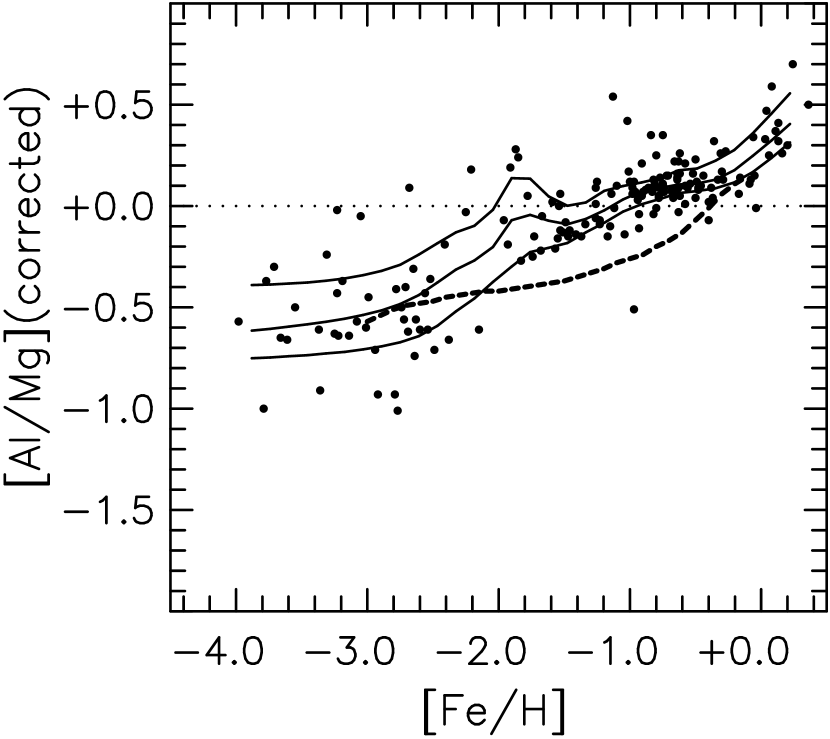
Figure 19:

Figure 20:

Figure 21:

Figure 22:

Figure 23:

Figure 24:

References

- (1)
- (2) Allende Prieto, C., Garcia López, R.J., Lambert, D.L., & Gustafsson, B. 1999, ApJ, 527, 879
- (3) Alonso, A., Arribas, S., & Martinez-Roger, C. 1996, A&A, 313, 873
- (4) Alonso, A., Arribas, S., & Martinez-Roger, C. 1999, A&AS, 140, 261
- (5) Anders, E. & Grevesse, N. 1989, Geochim. Cosmochim. Acta, 53, 197
- (6) Anstee, S.D. & O’Mara, B.J. 1995, MNRAS, 276, 859
- (7) Aoki, W., Norris, J.E., Ryan, S.G., Beers, T.C., & Ando, H. 2000, ApJ, 536, L97
- (8) Arpigny, C. & Magain, P. 1983, A&A, 127, L7
- (9) Asplund, M., Carlsson, M., Garcia Perez, A.E., & Kiselman, D. 2000, Proc. IAU GA 24, Joint Discussion 8, ed. B. Barbuy, in preparation
- (10) Asplund, M. & Nordlund, Å. 2000, Proc. IAU Symp. 198 The Evolution of the Light Elements, eds. L. da Silva, R. de Medeiros, & M. Spite, (San Francisco: ASP), in press
- (11) Asplund, M., Nordlund, Å., Trampedach, R., Stein, R.F., 1999, A&A, 346, L17
- (12) Barklem, P. S. & O’Mara, B. J. 1997, MNRAS, 290, 102
- (13) Barklem, P. S., O’Mara, B. J., & Ross, J. E. 1998, MNRAS, 296, 1057
- (14) Baumüller, D. & Gehren, T. 1997, A&A, 325, 1088
- (15) Beers, T.C., Flynn, K. & Gebhardt, K. 1990, AJ, 100, 32
- (16) Beers, T.C., Preston, G.W., & Shectman, S.A. 1985, AJ, 90, 2089
- (17) Beers, T.C., Preston, G.W., & Shectman, S.A. 1992, AJ, 103, 1987
- (18) Beers, T.C., Rossi, S., Norris, J.E., Ryan, S.G., Molaro, P., & Rebolo, R. 1998, Sp.Sci.Rev. 84, 139
- (19) Bell, R.A., Eriksson, K., Gustafsson, B., & Nordlund, Å. 1976, A&AS, 23, 37
- (20) Bell, R.A. & Gustafsson, B. 1978, A&AS, 34, 229
- (21) Bell, R.A. & Gustafsson, B. 1989, MNRAS, 236, 653
- (22) Bell, R.A. & Oke, J.B. 1986, ApJ, 307, 253
- (23) Bessell, M.S. 1979, PASP, 91, 589
- (24) Bessell, M.S. & Norris, J. 1984, ApJ, 285, 622
- (25) Bizzarri, A., Huber, M.C.E., Noels, A., Grevesse, N., Bergeson, S.D., Tsekeris, P., & Lawler, J.E. 1993, A&A, 273, 707
- (26) Blake, L.A.J., Ryan, S.G., Norris, J.E., & Beers, T.C. 2001, Nucl.Phys.A, in press
- (27) Boesgaard, A.M., King, J.R., Deliyannis, C.P., & Vogt, S.S. 1999, AJ, 117, 492
- (28) Bond, H.E. 1981, ApJ, 248, 606
- (29) Bonifacio, P., Molaro, P., Beers, T.C. & Vladilo, G. 1997, A&A, 332, 672
- (30) Buser, R. & Kurucz, R.L. 1992, A&A, 264, 557
- (31) Cardon, B.L., Smith, P.L., Scalo, J.M., Testerman, L., & Whaling, W. 1982, ApJ, 260, 395
- (32) Carney, B.W., Wright, J.S., Sneden, C., Laird, J.B., Aguilar, L.A., & Latham, D.W. 1997, AJ, 114, 363
- (33) Carr, B.J., Bond, J.R., & Arnett, W.D. 1984, ApJ, 277, 445
- (34) Cayrel, R., Andersen, J., Barbuy, B., Beers, T.C., Bonifacio, P., Francois, P., Hill, V., Molaro, P., Nordström, B., Plez, B., Primas, F., Spite, F., & Spite, M. 2000, Proc. IAU GA 24, Joint Discussion 8, ed. B. Barbuy, in preparation
- (35) Cayrel, R., Hill, V., Beers, T.C., Barbuy, B., Spite, M., Spite, F., Plez, B., Andersen, J., Bonifacio, P., Francois, P., Molaro, P., Nordström, B., & Primas, F. 2001, Nature, 409, 691
- (36) Cleveland, W.S. 1994, The Elements of Graphing Data (Revised Edition), ( Summit, NJ: Hobart Press)
- (37) Cottrell, P.L. & Norris, J. 1978, ApJ, 221, 893
- (38) Cowan, J.J., Pfeiffer, B., Kratz, K.-L., Thielemann, F.-K., Sneden, C., Burles, S., Tytler, D., & Beers, T.C. 1999, ApJ, 521, 194
- (39) Dessauges-Zavadsky, M., D’Odorico, S., McMahon, R.G., Molaro, P.,Ledoux, C., Peroux, C., Storrie-Lombardi, L.J., 2001, astro-ph/0102230
- (40) Fassia, A. & Meikle, W.P.S. 1999, MNRAS, 302, 314
- (41) Fassia, A., Meikle, W.P.S., Geballe, T.R., Walton, N.A., Pollaco, D.L., Rutten, R.G.M., & Tinney, C. 1998, MNRAS, 299, 150
- (42) Fryer, C.L., Woosley, S.E., & Heger, A. 2000, astro-ph/0007176
- (43) Fulbright, J.P. 1999, Ph.D. Thesis, Univ. of California Santa Cruz
- (44) Fulbright, J.P. 2000, astro-ph/0006260
- (45) Fulbright, J.P. & Kraft, R.P. 1999, AJ, 118, 527
- (46) Gibbons, J.D. 1985, Nonparametric Methods for Quantitative Analysis, 2nd Edition (Columbus: American Sciences Press)
- (47) Gilroy, K.K., Sneden, C., Pilachowski, C.A., & Cowan, J.J. 1988, ApJ, 327, 298
- (48) Gratton, R.G. 1989, A&A, 208, 171
- (49) Gratton, R.G., Carretta, E., Eriksson, K., & Gustafsson, B. 1999, A&A, 350, 955
- (50) Gratton, R.G. & Sneden, C. 1987, A&A, 178, 179
- (51) Gratton, R.G. & Sneden, C. 1988, A&A, 204, 193
- (52) Gratton, R.G. & Sneden, C. 1990, A&AS, 86, 269
- (53) Gratton, R.G. & Sneden, C. 1991, A&A, 241, 501
- (54) Gratton, R.G. & Sneden, C. 1994, A&A, 287, 927
- (55) Heger, A. & Woosley, S.E. 2000, ApJ, in preparation
- (56) Hill, V., Barbuy, B., Spite, M., Spite, F., Cayrel, R., Plez, B., Beers, T.C., Nordström B., & Nissen, P.E. 2000, A&A, 353, 557
- (57) Ikuta, C. & Aromoto, N. 1999, PASJ, 51, 459
- (58) Israelian, G., Garcia López, R.J., & Rebolo, R. 1998, ApJ, 507, 805
- (59) Israelian, G., Rebolo, R., Garcia López, R.J., Bonifacio, P., Molaro, P., Basri, G., & Shchukina, N. 2001, astro-ph/0101032
- (60) Karamatskos, N., Michalak, R., Zimmermann, P., Kroll, S., & Kock, M. 1986, Z.Phys.D, 3, 391
- (61) Kraft, R.P., Suntzeff, N.B., Langer, G.E., Carbon, D.F., Trefzger, C.F., Friel, E., & Stone, R.P.S. 1982, PASP, 94, 55
- (62) Kurucz, R.L. 1970, SAO Special Report No. 309
- (63) Kurucz, R.L. 1993, CD-ROM 13, ATLAS Stellar Atmospheres Programs and 2 km/s grid (Cambridge: Smithsonian Astrophysical Obs.)
- (64) Lambert, D.L. 1978, MNRAS, 182, 249
- (65) Langer, G.E., Kraft, R.P., Carbon, D.F., Friel, E., & Oke, J.B. 1986, PASP, 98, 473
- (66) Lawler, J.E. & Dakin, J.T. 1989, J.Opt.Soc.Am.B, 6, 1457
- (67) Maeder, A. 1997, in Abundance Profiles: Diagnostic Tools for Galaxy History, ASP Conf. Ser. Vol. 147, eds. D. Friedli, M. Edmunds, C. Robert, & L. Drissen (San Francisco: ASP), 224.
- (68) McWilliam, A. 1990, ApJS, 74, 1075
- (69) McWilliam, A. 1998, AJ, 115, 1640
- (70) McWilliam, A., Preston, G.W., Sneden, C., & Searle, L.. 1995b, AJ, 109, 2757
- (71) McWilliam, A., Preston, G.W., Sneden, C., & Shectman, S. 1995a, AJ, 109, 2736
- (72) Molaro, P. & Bonifacio, P. 1990, A&A, 236, L5
- (73) Molaro, P. & Castelli, F. 1990, A&A, 228, 426
- (74) Nakamura, T., Umeda, H., Iwamoto, K., Nomoto, K., Hashimoto, M., Hix, W.R., & Thielemann, F.-K. 2000. astro-ph/0011184
- (75) Nakamura, T., Umeda, H., Nomoto, K., Thielemann, F.-K., & Burrows, A. 1999, ApJ, 517, 193
- (76) Nissen, P.E. & Schuster, W.J. 1997, A&A, 326, 751
- (77) Nitz, D.E., Kunau, A.E., Wilson, K.L., & Lentz, L.R. 1999, ApJS, 122, 557
- (78) Norris, J.E. 1999, The Third Stromlo Symposium: The Galactic Halo, eds. B.K.Gibson, T.S. Axelrod, and M.E.Putman (San Francisco: ASP), 213
- (79) Norris, J.E., Beers, T.C., & Ryan, S.G. 2000, ApJ, 540, 456
- (80) Norris, J.E., Peterson, R.C., & Beers, T.C. 1993, ApJ, 415, 797
- (81) Norris, J.E., Ryan, S.G., & Beers, T.C. 1996, ApJS, 107, 391
- (82) Norris, J.E., Ryan, S.G., & Beers, T.C. 1997a, ApJ, 488, 350
- (83) Norris, J.E., Ryan, S.G., & Beers, T.C. 1997b, ApJ, 489, L169
- (84) Pettini, M., Smith, L.J., King, D.L., & Hunstead, R.W. 1997, ApJ, 486, 665
- (85) Preston, G.W., Shectman, S.A., & Beers, T.C. 1991, ApJS, 76, 1001
- (86) Primas, F., Molaro, P., Bonifacio, P., & Hill, V. 2000, astro-ph/0008402
- (87) Primas, F., Molaro, P., & Castelli, F. 1994 A&A, 290, 885
- (88) Prochaska, J. X. & Wolfe, A. M. 1999, ApJS, 121, 369
- (89) Rossi, S., Beers, T.C., & Sneden, C. 1999, The Third Stromlo Symposium: The Galactic halo, ASP Conf. Ser. 165, eds. B.K. Gibson, T.S. Axelrod, & M.E. Putman, (San Francisco: ASP), 264
- (90) Ryan, S. G. 1998, A&A, 331, 1051
- (91) Ryan, S.G., Aoki, W., Blake, L.A.J., Norris, J.E., Beers, T.C., Gallino, R., Busso, M., & Ando, H. 2001, Mem.S.A.It., in press
- (92) Ryan, S.G., Beers, T.C., Olive, K.A., Fields, B.D., & Norris, J.E. 2000, ApJ, 530, L57
- (93) Ryan, S.G., Norris, J.E., & Beers, T.C. 1996, ApJ, 471, 254
- (94) Ryan, S.G., Norris, J.E., & Beers, T.C. 1999, ApJ, 523, 654
- (95) Ryan, S.G., Norris, J.E., & Bessell, M.S. 1991, AJ, 102, 303
- (96) Shigeyama, T. & Tsujimoto, T. 1998, ApJ, 507, L135
- (97) Sneden, C., McWilliam, A., Preston, G.W., Cowan, J.J., Burris, D.L., & Armosky, B.J. 1996, ApJ, 467, 819
- (98) Sneden, C. & Parthasarathy, M. 1983, ApJ, 267, 757
- (99) Songaila, A. & Cowie, L.L. 1996, AJ, 112, 335
- (100) Stephens, A. 1999, AJ, 117, 1771
- (101) Thévenin, F. & Idiart, T.P. 1999, ApJ, 521, 753
- (102) Timmes, F.X., Woosley, S.E., & Weaver, T.A. 1995, ApJS, 98, 617
- (103) Tomkin, J., Lemke, M., Lambert, D.L., & Sneden, C. 1992, AJ, 104, 1568
- (104) Tomkin, J., Woolf, V.M., Lambert, D.L., & Lemke, M. 1995, AJ, 109, 2204
- (105) Travaglio, C., Gallino, R., Amari, S., Zinner, E., Woosley, S., & Lewis, R.S. 1999, ApJ, 510, 325
- (106) Tsujimoto, T. & Shigeyama, T. 1998, ApJ, 508, L151
- (107) Tsujimoto, T., Shigeyama, T., & Yoshii, Y. 1999, ApJ, 519, L63
- (108) Umeda, H., Nomoto, K., & Nakamura, T. 2000, The First Stars, ESO Conf., eds. A. Weiss, T. Abel, & V. Hill (Berlin: Springer), 149
- (109) Woosley, S.E. & Weaver, T.A. 1982, Supernovae: A Survey of Current Research, eds. M.J. Rees & R.J. Stoneham (Dordrecht: Reidel), 79
- (110) Woosley, S.E. & Weaver, T.A. 1995, ApJS, 101, 181
- (111)