Measurement of the Crab Flux above 60 GeV with the CELESTE Čerenkov Telescope

Abstract

We have converted the former solar electrical plant THEMIS (French Pyrenees) into an atmospheric Čerenkov detector called CELESTE, which records gamma rays above $30\mathrm{\ GeV}$ ($7\times 10^{24}\mathrm{\ Hz}$). Here we present the first sub-$100\mathrm{\ GeV}$ detection by a ground based telescope of a gamma ray source, the Crab nebula, in the energy region between satellite measurements and imaging atmospheric Čerenkov telescopes. At our analysis threshold energy of $60\pm 20\mathrm{\ GeV}$ we measure a gamma ray rate of $6.1\pm 0.8$ per minute. Allowing for 30% systematic uncertainties and a 30% error on the energy scale yields an integral gamma ray flux of

$$I(E>60\mathrm{\ GeV})=6.2^{+5.3}_{-2.3}\times 10^{-6}\mathrm{\ photons}\mathrm{\ m^{-2}}\mathrm{\ s^{-1}}.$$

The analysis methods used to obtain the gamma ray signal from the raw data are detailed. In addition, we determine the upper limit for pulsed emission to be ¡12% of the Crab flux at the 99% confidence level, in the same energy range. Our result indicates that if the power law observed by EGRET is attenuated by a cutoff of form $e^{-E/E_{0}}$ then $E_{0}<26\mathrm{\ GeV}$. This is the lowest energy probed by a Čerenkov detector and leaves only a narrow range unexplored beyond the energy range studied by EGRET.

1 Introduction

The Crab was the first source of gamma rays to be convincingly detected by ground based telescopes (Weekes et al., 1989; Vacanti et al., 1991) and measurements of its emission spectrum between $250\mathrm{\ GeV}$ and $20\mathrm{\ TeV}$ by various atmospheric Čerenkov detectors are now available (Hillas et al., 1998; Aharonian et al., 2000; Piron et al., 2000; Masterson et al., 2001). The flux measurement above $190\pm 60\mathrm{\ GeV}$ recently reported by the STACEE experiment, using the mirrors of a solar energy research facility to collect Čerenkov light, is the first detection below 200 GeV by a ground based device (Oser et al., 2001). At these energies emission from the Crab is steady and generally accepted to come from the nebula, arising from the inverse Compton scattering of the synchrotron photons observed at lower energies (Gould, 1965; de Jager & Harding, 1992).

The EGRET detector on board the Compton Gamma Ray Observatory was used to study the Crab from $0.03$ to $10\mathrm{\ GeV}$ (Fierro et al., 1998). The differential energy spectrum measured by EGRET is well described by the sum of two power laws. Below $0.1\mathrm{\ GeV}$ the steep spectrum is attributed to the synchrotron radiation from the nebula, while beyond $0.1\mathrm{\ GeV}$ the spectrum hardens and is dominated by pulsed emission. The detailed origin of the pulsar emission is uncertain. The outer gap (Cheng, Ho & Ruderman, 1986; Romani & Yadigaroglu, 1995; Hirotani & Shibata, 2000) and polar cap (Daugherty & Harding, 1982) models offer differing pictures. Current very high energy measurements create difficulties for some outer gap models (Lessard et al., 2000) but refining the picture requires observations in the heretofore uncovered $10-200\mathrm{\ GeV}$ region. Determining the energy at which pulsed emission is again overtaken by the nebula flux is one of the goals of the present work.

While the Crab itself is a rather special object, the success of the synchrotron self-Compton (SSC) model as applied to the nebula has wide implications. On the one hand, this bright source is a test piece for the study of supernova remnants as the acceleration sites of high energy cosmic rays, with at issue the question of whether proton or electron acceleration dominates in a given source. In addition, the SSC mechanism is a cornerstone for the interpretation of the broadband spectra of AGNs of the blazar class (Dermer & Schlickeiser, 1993; Ghisellini & Maraschi, 1996; Marcowith et al., 1995). The experimental data from the Crab which support the SSC picture consist of EGRET flux measurements up to $10\mathrm{\ GeV}$, with large uncertainties in the region above $1\mathrm{\ GeV}$ (de Jager et al., 1996), and the extrapolation across more than a decade in energy to the spectra measured by the atmospheric Čerenkov experiments. Clearly, an independent measurement in the intervening $50\mathrm{\ GeV}$ region ($1.2\times 10^{25}\mathrm{\ Hz}$) where the inverse Compton peak in the power spectrum is expected to lie would further constrain the parameters of this important model.

The minimum energy threshold, $E_{thresh}$, for current ground based imaging atmospheric Čerenkov experiments is limited to $\sim 200\mathrm{\ GeV}$ by the rate of accidental triggers due to the night sky light and, in the case of single mirror experiments, by the rate of local muon triggers. The simplest way to reduce the threshold of such an experiment is to increase the available mirror area, $A$, as $E_{thresh}\propto\sqrt{1/A}$; an approach which is being followed by the MAGIC collaboration (Martinez et al., 1999). Alternatively, an array of smaller telescopes can be used to reach thresholds of $\sim 100\mathrm{\ GeV}$ as predicted for the VERITAS (Bradbury et al., 1999) and HESS (Kohnle et al., 1999) experiments. These experiments are currently under construction and have not yet started taking data.

CELESTE was designed to reach a very low energy threshold without a large expenditure of time and resources by exploiting the mirrors of an existing structure; a de-commissioned solar farm in the French Pyrenees. An array of 40 such mirrors, used by CELESTE to sample the arrival time and photon flux of the Čerenkov wave front at intervals of $\sim 30\mathrm{\ m}$, provides a total mirror area of $\sim 2000\mathrm{\ m^{2}}$. CELESTE uses techniques similar to those pioneered by the early wavefront sampling experiments ASGAT (Goret et al., 1993) and THEMISTOCLE (Baillon et al., 1993) which operated on the same site, but uses a much greater mirror area and more sophisticated trigger logic and data acquisition electronics. Unlike the imaging experiments, the wavefront sampling method gives no direct information about the shower morphology, but alternative methods of hadron rejection can be developed using the shape of the wavefront and the distribution of Čerenkov light on the ground. Since their Crab detection cited above, STACEE has lowered their threshold to $120\pm 25\mathrm{\ GeV}$ and expects to descend to $70\mathrm{\ GeV}$ (Covault et al., 2001). The GRAAL experiment also uses a heliostat array but without secondary optics obtains a relatively high threshold of $250\pm 110\mathrm{\ GeV}$ (Arqueros et al., 2001).

In this paper we present the first measurement of the flux from the Crab above $60\mathrm{\ GeV}$, as well as an upper limit for pulsed emission, using the CELESTE heliostat array. We begin with a description of the experiment followed by a summary of the data sample and observation techniques. CELESTE exploits a new experimental technique so we outline the analysis method in some detail, including the results of extensive Monte Carlo simulations of the detector and the analysis of data taken in common with the CAT imaging Čerenkov telescope. The gamma ray flux measurement and the pulsed flux upper limit are presented and the implications for the emission models are discussed. Further details on these measurements and on the CELESTE experiment in general are available in de Naurois (2000).

2 The CELESTE Experiment

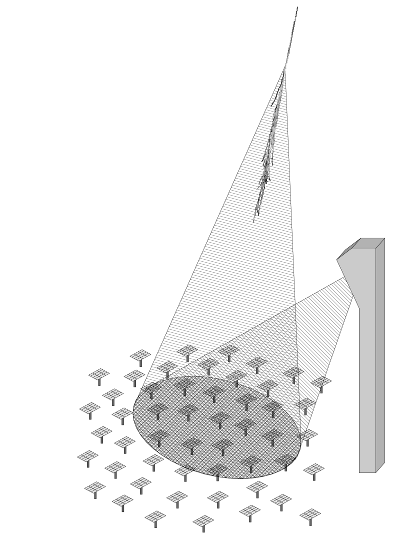
Figure 1: Principle of the experimental apparatus. As the heliostats track a source they reflect Cherenkov light generated by atmospheric particle cascades to the secondary optics and photomultipliers located near the top of the 100 meter tall tower.

The CELESTE experiment is described in full detail in the experiment proposal (Smith et al., 1996) and in (Reposeur et al., 2001). Here we outline the most important features and the status of the experiment during the relevant observation period. Fig. 1 illustrates the experimental principle.

CELESTE uses 40 heliostats of a former solar electrical plant at the Thémis site in the eastern French Pyrénées (N. $42.50^{\circ}$, E. $1.97^{\circ}$, altitude $1650\mathrm{\ m}$). Each back-silvered heliostat mirror has an area of $54\mathrm{\ m^{2}}$ and moves on an alt-azimuth mount. The heliostats are controlled from the top of a $100\mathrm{\ m}$ tall tower, located south of the heliostat field, which houses the secondary optics, photomultiplier tubes (PMTs) and data acquisition system. The alignment of the heliostats has been verified by mapping the images of bright stars using the PMT anode current.

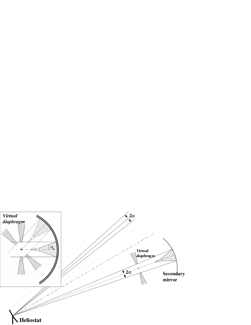
Figure 2: The CELESTE secondary optics. Winston cones define a “virtual diaphragm” which limits the geometrical field of view to $2\alpha=10$ mrad (figure not to scale).

The light from all 40 heliostats is reflected to the top of the tower. To separate these signals from each other we use a secondary optical system, as illustrated in Fig. 2. We have chosen to place the photomultiplier assembly on the optical axis to minimize coma aberrations, although this results in a loss of light due to the shadow formed. The spherical mirrors of the secondary optics are divided into six segments on three levels with three different focal lengths in order to reduce this shadowing effect and to produce images of approximately the same size regardless of the heliostat position in the field. One large segment views the farthest heliostats, two others view those at intermediate distance, and three small segments are used for the heliostats at the foot of the tower. At the secondary mirror focus is the entrance face of a solid Winston cone glued to a two-inch PMT (Philips XP2282B), one for each heliostat. The Winston cone determines the surface area of the secondary mirror seen by that PMT, such that the optical field-of-view of each tube is $2\alpha=10$ mrad (full width). This field-of-view is slightly smaller than the angular size of air showers in our energy range and helps maximze the ratio of Čerenkov to night sky light.

The single photoelectron (PE) pulse width, after pre-amplifiers (gain=100, AC-coupled) and 23 m cables to the counting house, is just under $5\mathrm{\ ns}$ (full width at half maximum). PMT gains are set reasonably low ($\sim 5\times 10^{4}$) to avoid damage to the tubes from night sky light, and the electronic gains are such that the amplitude of a single photoelectron in the counting house is $10\mathrm{\ mV}$ on average. These amplitudes were measured in situ. In fact, studies of the average response of each detector to the hadronic background events have enabled us to calibrate the relative efficiency of each heliostat, and the PMT high voltages are now set so as to correct for this (in the range $\sim\pm 25\%$) in order to give an even trigger response across the heliostat field. The PMT signals are sent to both the trigger electronics and to the data acquisition system.

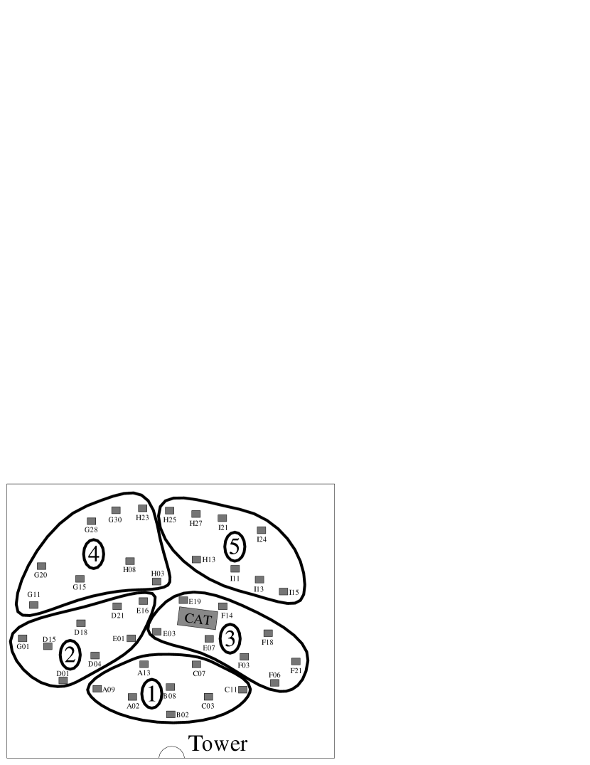
Figure 3: The division of the heliostat field into 5 trigger groups, each of 8 heliostats.

The trigger is designed to reach the lowest possible threshold. Programmable analog delays compensate for the changing optical path lengths as the source direction changes during the observation. The switched-cable delays broaden the PE pulse widths by a full nanosecond for the maximum delay. Eight PMT signals are summed in each of five groups as shown in Fig. 3, and the sums enter a discriminator. Programmable logic delays further compensate for the varying path lengths between the trigger groups. The logic delay introduces a deadtime of the order of 5%. A trigger requires the logic coincidence of at least three of the five groups, with an overlap of $10\mathrm{\ ns}$. The analog sum over eight heliostats provides us with a good signal to noise ratio for the Čerenkov pulse, while the logic coincidence removes triggers due to afterpulsing in the PMTs, local muons or low energy hadronic events illuminating only a few heliostats.

Each PMT signal is further amplified ($\times 2$) and sent to an 8-bit Flash ADC (FADC) circuit (Etep 301c) that digitizes the signal at a rate of $0.94\mathrm{\ GHz}$ (1.06 ns per sample). The depth of the FADC memory is 2.2 $\mu$s, and one photoelectron corresponds to 3 digital counts. When a trigger occurs, digitization stops and a window of 100 samples centered at the nominal Čerenkov pulse arrival time is read out via two VME busses in parallel. Readout requires $7\mathrm{\ ms}$, which for typical raw trigger rate of 25 Hz gives an acquisition deadtime fraction of $20\mathrm{\ \%}$. The trigger also latches a GPS clock, which is read out and included in the data stream. In parallel with the Čerenkov pulse data acquisition, scalers record the single group trigger rates, the final trigger rate, and the readout rate. Acquisition deadtime is determined from the latter two. The anode current of each PMT ($\sim 10~{}\mu\mathrm{A}$) is also recorded, as is some meteorological information.

3 Crab Observations

The observations presented here were taken on clear, moonless nights during the Crab season between November 1999 and March 2000. All the data were taken when the source was within 2.5 hours of transit, that is, with an angle from the zenith, $\Theta<40^{\circ}$. The observations were made in the ON-OFF tracking mode, in which an observation of the source is followed or preceded by an observation at the same declination offset in right ascension by an appropriate amount (usually 20 minutes). The offset region is then used as a reference to provide a measure of the background of cosmic ray events. It is particularly important in the case of CELESTE to cover the same elevation and azimuth ranges during the ON and the OFF source observations as the heliostat optical collection efficiencies change appreciably due to the projection of the heliostat surface viewed by the PMTs, and (less importantly) due to optical aberrations. Both of these effects depend upon the heliostat orientation and thus upon the source direction. In addition, matching ON and OFF source observations ensures that the ON and OFF data were taken using exactly the same path through the delay electronics.

CELESTE has a number of options when deciding how to observe a source. The majority of the data here were taken in “single pointing”, wherein all the heliostats were aimed at a point $11\mathrm{\ km}/\cos\Theta$ upward from the center of the heliostat field towards the source such that the center of their fields of view converged at the expected maximum point of Čerenkov emission for gamma showers. This method collects the largest number of photons, allowing us to operate with the lowest possible energy threshold. It seems likely, however, that other pointing strategies may provide better sampling across the shower and hence better hadron rejection. With this in mind, a smaller number of runs were taken using “double pointing” in which half the heliostats pointed at $11\mathrm{\ km}/cos\Theta$, and the other half at $25\mathrm{\ km}/\cos\Theta$. A Monte Carlo study of some different pointing methods is available in Herault (2000). The observing log is summarised in Table 1.

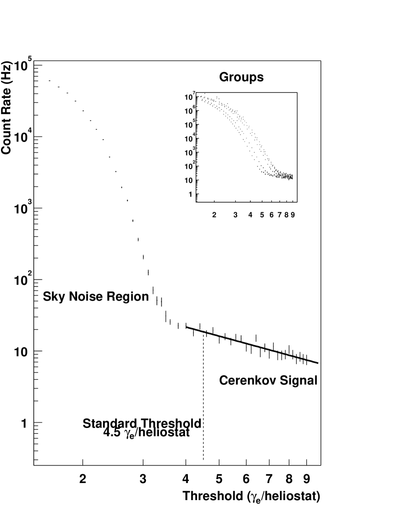
Figure 4: The total trigger rate as a function of discriminator threshold per heliostat for a particularly clear dark night. Inset: the rates for each of the 5 trigger groups as a function of their discriminator levels, in photoelectrons ($\gamma_{e}$) per heliostat.

The trigger logic was set such that 3 groups out of the 5 were required to exceed their discriminator threshold in order to trigger the experiment. The discriminator threshold levels for each of the 5 trigger groups are checked nightly by measuring the trigger rate as a function of discriminator level in order to find the break point between accidental coincidences of random noise pulses and Čerenkov flashes. We set the discriminators such that the noise triggers contribute less than 1% of the total rate (Fig. 4). For more than 90% of the Crab data the discriminator level was set to $360\mathrm{\ mV}$, that is, an average of $4.5\mathrm{\ PE}$ for each of the 8 heliostats in a group, giving a final trigger rate of $\sim 25\mathrm{\ Hz}$. Expressing the discriminator level for the analog sum of 8 heliostats in a group in terms of PE per heliostat implies that the Cerenkov pulses for each heliostat are perfectly in time with each other. We have checked this timing by reconstructing the group sums using the FADC data (although the path to the trigger electronics is not identical to the acquisition path) and by oscilloscope measurements during observations. For the data in this paper, three channels were as much as 2 ns out of time, while the other 37 channels were less than 1 ns from the average. The three outlying channels have since been corrected, and the group sum pulses are now routinely digitized using additional FADCs.

The PMT anode current information and the measured trigger rates of each group are very sensitive to changes in the sky conditions and are used to verify that the atmosphere was stable throughout the ON-OFF pair. Any data which showed evidence of poor weather or equipment problems were rejected. The remaining total data set consists of 14.3 hours of ON-source exposure.

4 Analysis

Here we outline the important stages in the analysis of CELESTE data; data cleaning, shower reconstruction and hadronic background rejection. We also present the results of extensive Monte Carlo simulations which have been used to derive the analysis techniques and to estimate the sensitivity and threshold of the experiment. CELESTE has the advantage of being situated on the same site as a well calibrated atmospheric Čerenkov imaging telescope, CAT (Barrau et al., 1998). This has allowed us to examine the collection efficiency for a subset of the CELESTE data and should in the future allow us to cross-calibrate energy, direction, and acceptance between CAT and CELESTE.

4.1 Pre-analysis

For each event which triggers CELESTE, we record a window of $106\mathrm{\ ns}$ around the Čerenkov pulse for each PMT using FADCs with a sampling period of $1.06\mathrm{\ ns}$ (i.e. 100 samples). The FADC window is chosen such that the Čerenkov pulse is expected to arrive in its center. The beginning of the FADC window (the first 30 samples) is used to calculate the pedestal level. A small constant voltage offset applied to the unipolar input of each FADC allows fluctuations in the night sky background to be measured. Significant differences in the amplitude $\sigma_{p}$ of these fluctuations can be seen depending upon the brightness of the region of sky viewed by the PMT.

The possibility of systematic effects in the data due to differences in night sky background levels between the ON and OFF source regions of the sky is a known problem for atmospheric Čerenkov experiments. Cawley (1993) proposed a method of “software padding”, for use with the Whipple telescope, in which the noise fluctuations of the ADC signals from the darker region of sky are artificially increased to the same level as the brighter region by adding from a randomly sampled Gaussian distribution. The effects of night sky light differences can be seen at both the trigger level and in parameter distributions during the analysis procedure. These systematic effects produce a significant difference between the number of events remaining from the ON source and OFF source regions after analysis cuts. The difference can be either positive or negative, depending on which region is the brighter, and a positive difference mimics a real signal. CELESTE is particularly prone to these problems due to its large mirror area and angular acceptance per PMT which combine to give a night sky light background rate of $\sim 1\mathrm{\ PE}/\mathrm{\ ns}$. The use of FADCs introduces another complication in the case of CELESTE: if we wish to extract more information than just the integrated charge over the pulse, a simple addition of charge sampled from a night sky background distribution to the measured charge is not sufficient. The effect of additional sky noise on the complete Čerenkov pulse shape must be accounted for. The only way to equalize the night sky background fluctuations in software then, is to simulate the response of the PMT-FADC electronics chain to an increased rate of single photo-electrons.

We model the single PE pulse using events triggered by cosmic ray muons passing through the Winston cones, in standard operating conditions except with the tower door closed, blocking outside light. These pulses contain many ($\sim 50$) PEs, generated at the photocathode at almost exactly the same time so to a good approximation the muon pulse shape is the same as that of a single PE, only of greater amplitude. The results agree with those obtained on a test bench with an oscilloscope, and with single PE pulses measured by the FADC’s, using much higher PMT gains which change the PMT time response somewhat. By simulating the FADC response to single PEs arriving at different rates, we obtain a calibration curve of measured fluctuation against the background rate of PEs due to night sky light of the form $\sigma_{p}=s\sqrt{b}$ where $s$ is a constant and $b$ is the night sky background rate in $\mathrm{\ PE}$ per ns. This curve can be used to calculate the rate of simulated PEs which needs to be added to the darker field in order to equalize the night sky background fluctuations.

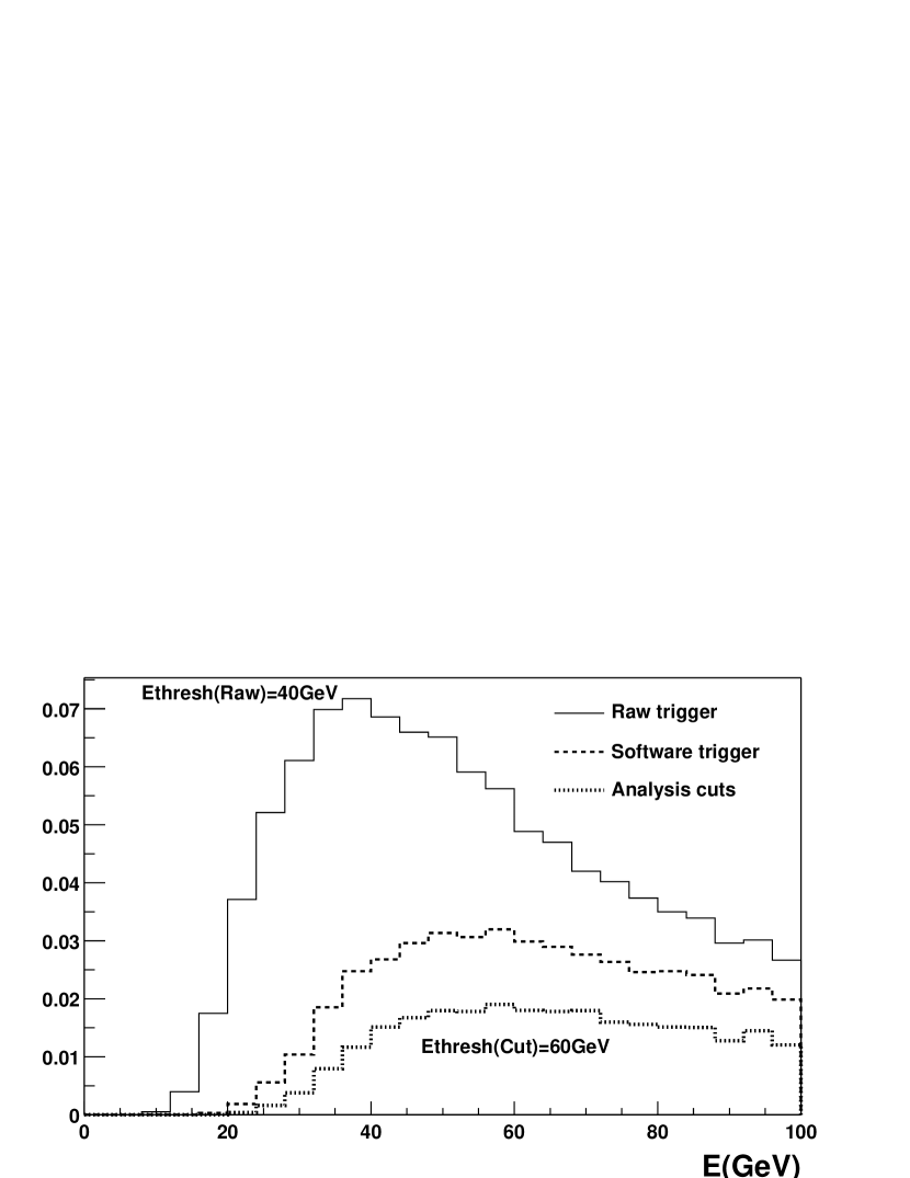
Figure 14: The simulated response of CELESTE to an $E^{-2}$ power law gamma ray spectrum (normalized to the integral of the raw trigger curve). The gamma rays have been simulated with the same distribution of azimuth and zenith angles as the 11 km Crab observations. The analysis cuts are $N_{\mathrm{peaks}}\geq 10$ and $\sigma_{\mathrm{grp}}<0.25$.

Software padding has been applied to all the ON-OFF pairs used in this analysis but this alone is not sufficient to remove all the biases caused by night sky background differences as a brighter region of sky also causes a slight increase in the amount of near threshold events which trigger the experiment. This can be explained as follows: additional night sky background fluctuations cause showers which would otherwise be below threshold to trigger. They also prevent some events which would otherwise be above threshold from triggering, but because the cosmic ray spectrum is very steep, the former effect is bigger than the latter, and there is a net night sky background dependent increase in the number of triggered events. We have therefore found it necessary to apply a “software trigger” at a level higher than the hardware trigger level, in order to remove these additional small events. Using the FADC data, we reconstruct the analog sum pulses seen by each of the five trigger groups and then apply the condition: $\geq$4 groups $>5.0\mathrm{\ PE}$ per heliostat. This provides us with comparable background data in the ON and OFF fields, and reduces the fraction of events triggered by accidental noise coincidences to less than $10^{-3}$, but has the effect of increasing the energy threshold of the experiment (Fig. 14).

To test the performance of the software trigger, we have divided the Crab data set into two subsets, based on the sign of the difference in the average PMT currents between the ON and OFF source observations. Fig. 5 shows the difference between the ON and OFF source observations for the distribution of the total charge measured in all the Čerenkov pulses for these two subsets. A clear bias in the number of small events is apparent in the raw data, with the direction of the bias depending upon the sign of the current difference. After application of the software trigger, the bias has been removed.

In order to use the information recorded by the FADCs, it is necessary to select and parameterize the Čerenkov peaks. This is done by fitting a function of the following form:

$$f(t)=\left\{\vbox{\hbox{\hbox to85.35826pt{$\displaystyle Pe^{\frac{-(t-t_{0})^{2}}{2\sigma_{l}^{2}}}$}\quad for \quad$t\leq t_{0}$} \vspace{0.5em} \hbox{\hbox to85.35826pt{$\displaystyle Pe^{\frac{-|t-t_{0}|}{\sigma_{r}}}$}\quad for \quad$t>t_{0}$} \vspace{0.3em}}\right.$$ (1)

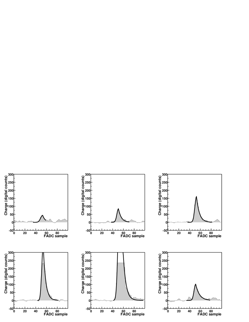
Figure 6: An example of the peak finding and fitting algorithm for a series of Čerenkov signals of various amplitudes. The 100 sample FADC data window is plotted in digital counts against FADC sample number.

where $t$=time in nanoseconds, $t_{0}$=peak time and $P$=peak amplitude. Fig. 6 shows some examples of fitted peaks and illustrates the effect of saturation in the FADCs. Studies using simulated peaks indicate that the peak fitting algorithm can accurately reconstruct the timing and charge information for peaks which have saturated the FADCs up to twice their dynamic range. The fit parameters for each peak are stored for use later in the analysis. Only events having at least 10 Čerenkov peaks with an amplitude greater than 25 digital counts ($\simeq 8$ P.E.) are used in the analysis ($N_{\mathrm{peaks}}\geq 10$).

4.2 Analysis Strategy

Imaging Čerenkov telescopes have become the most powerful instruments at energies greater than $200\mathrm{\ GeV}$ due to their efficiency in reducing the hadronic background. Typically, it is possible to reject over 99% of the background events while retaining 50% of the gamma ray signal (Punch et al., 1991). At CELESTE energies, a smaller total number of photons and intrinsic fluctuations in the shower development mean that the differences between the gamma and hadron showers which trigger are less pronounced. In addition the small field of view of CELESTE, which is necessary to keep the night sky light background at a reasonable level, often truncates the shower, again causing hadron and gamma showers to look alike. These points, and also the fact that the trigger system rejects many hadron showers at the hardware level, mean that hadron rejection at the analysis stage is not very efficient for CELESTE; however, small differences do remain, as the gamma showers tend to develop in a more regular manner than the hadron showers.

We have written a complete detector simulation package, including a full treatment of the complicated optical system of CELESTE and a detailed model of the trigger and acquisition electronics, for use with standard air shower simulation packages. Using the Monte Carlo simulations we have investigated various ways of exploiting the FADC timing and charge information to provide hadron rejection. Two rather simple parameters have been studied in detail: the group homogeneity, $\sigma_{grp}$, and the shower axis angle, $\theta$.

The group homogeneity is a measure of the homogeneity of the Čerenkov light pool at ground level. It is determined from the variance in the amplitude of the five trigger group pulses normalized to the mean amplitude. The trigger group pulses are derived by summing the 8 FADC windows of the heliostats in each group.

$$\sigma_{\mathrm{\scriptstyle grp}}=\frac{\sqrt{\big{<}A_{\mathrm{grp}}^{2}\big{>}-\big{<}A_{\mathrm{grp}}\big{>}^{2}}}{\big{<}A_{\mathrm{grp}}\big{>}}$$ (2)

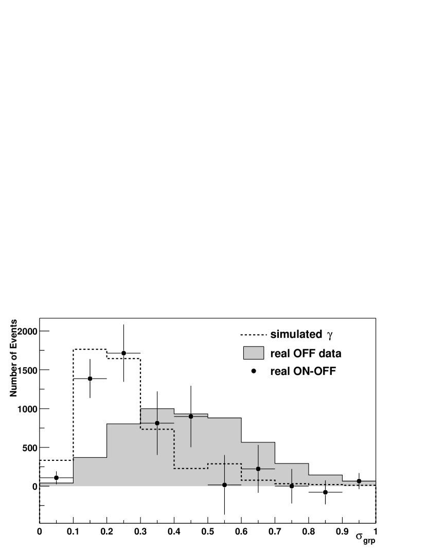
Figure 7: The distribution of $\sigma_{grp}$, a measure of the homogeneity of the light distribution at the ground, for simulated gamma rays, OFF source data and for the difference between the ON and OFF source data after the software trigger and with $N_{\mathrm{peaks}}\geq 10$. The distributions are normalized to this measured excess.

where $A_{grp}$ are the amplitudes of the 5 reconstructed trigger group pulses. Fig. 7 shows the distribution of $\sigma_{grp}$ for gamma rays and OFF source data after applying the software trigger and requiring a minimum of 10 Čerenkov peaks. The gamma rays were simulated over a range of azimuth and zenith angles so as to match the range covered by all the data for the $12.1\mathrm{\ hour}$ Crab data set described in Table 1. The OFF source data shown is the sum of all the OFF source data in this data set. According to this plot, a cut at $\sigma_{\mathrm{\scriptstyle grp}}\leq 0.25$ conserves $61\%$ of the gammas which remain after the software trigger, while rejecting $85\%$ of the remaining hadrons, giving a quality factor Q=1.6 where:

$$Q=\frac{\hbox{eff}_{\gamma}}{\sqrt{\hbox{eff}_{\hbox{\scriptsize hadrons}}}}$$ (3)

and $\mathrm{eff}_{\gamma}$ and $\mathrm{eff}_{hadrons}$ are the fraction of gammas and hadrons conserved by the cut respectively.

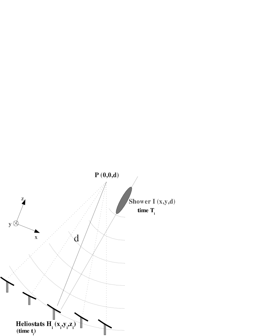
Figure 8: An illustration of the shower maximum reconstruction. $P$ is the point being tracked, $H_{i}$ are the heliostat positions, $I$ is the position to be calculated.

Low energy gamma ray air showers are only a few kilometres long and the majority of the Čerenkov light is emitted from a small region. The Čerenkov wavefront is therefore spherical to a good approximation (Fig. 8). Using the arrival times of the Čerenkov pulses we are able to reconstruct this wavefront using an analytical $\chi^{2}$ minimization procedure (de Naurois, 2000).

Assuming that the point of emission was at a fixed distance $d=11\mathrm{\ km}/\cos{\Theta}$ from the site towards the source, the fit gives the position $I(x,y,d)$ of the shower maximum relative to the tracked point, $P(0,0,d)$. Simulations indicate that this position is reconstructed with an error of $\sigma(\sqrt{x^{2}+y^{2}})\approx 15\mathrm{\ m}$.

It is important to know the timing resolution for each detector when making the fit. We have calculated this resolution by studying the response to a nitrogen laser pulse sent to a diffuser mounted at the top of the tower. The same laser was used for a similar purpose by the THEMISTOCLE experiment on the same site (Baillon et al., 1993). The timing resolution is also dependent upon the background night sky light level and on the amplitude of the pulse. This dependency is difficult to test with the laser so we have measured it by generating simulated peaks, adding them to real night sky background data and then comparing the reconstructed peak time with the known injection time of the simulated peak. The resolution reaches $\sim 0.6$ ns for peaks well above the night sky noise level, and is worse for larger and smaller peaks due to FADC saturation and relatively larger night sky fluctuations, respectively.

Using the expected point of maximum emission we can attempt to measure the angle, $\theta$, of the shower axis relative to the pointing direction, which will be zero in the case of gamma rays originating from a point source at the center of the field of view. To do this we need a second point at ground level, simply calculated by taking the mean position of the heliostats on the ground, weighted by the charge sampled by each detector. More complex algorithms have been tested for calculating the impact parameter, but none has proved more effective than this simple method, which gives a $1~{}\sigma$ error of $\sim 30\mathrm{\ m}$ according to the simulations.

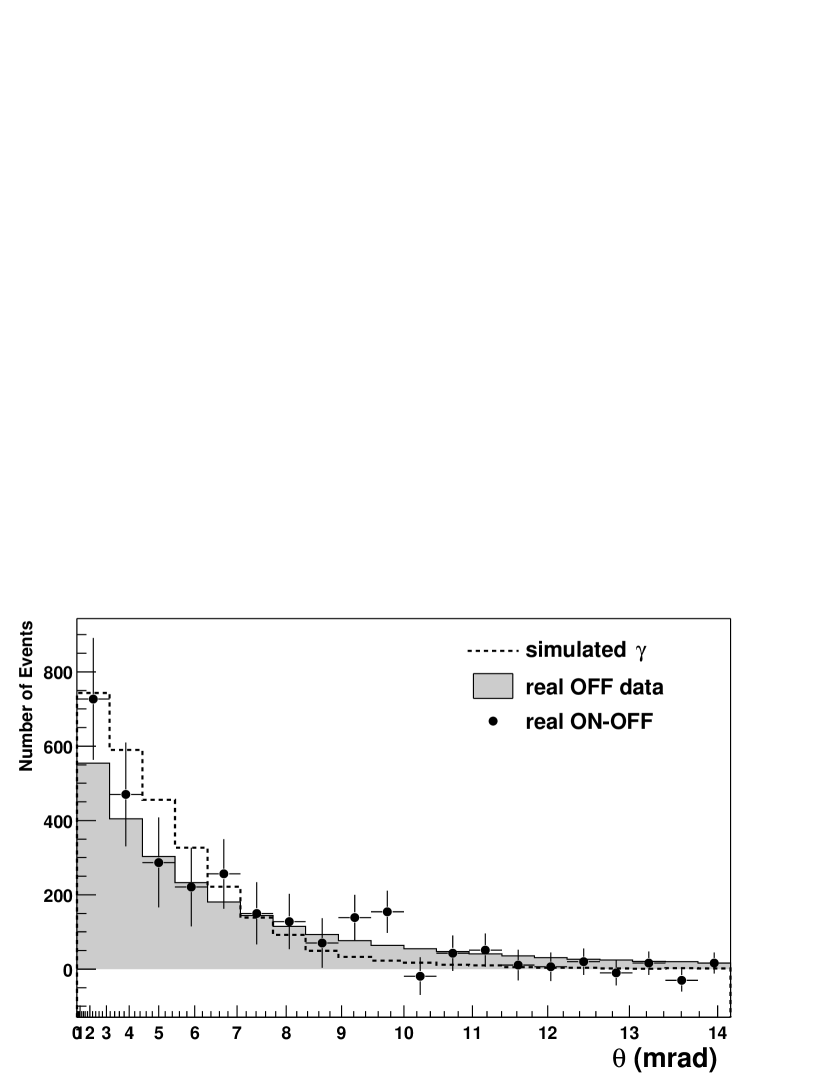
Figure 9: The distribution of $\theta$, the shower axis angle relative to the source direction, for simulated gamma rays, OFF source data and for the difference between the ON and OFF source data after the software trigger, with $N_{\mathrm{peaks}}\geq 10$ and $\sigma_{\mathrm{grp}}<0.25$. The distributions are normalized to this measured excess. The scale is quadratic.

The distribution of $\theta$ for simulated gammas and for real OFF source data after the software trigger, requiring a minimum of 10 Čerenkov peaks and $\sigma_{grp}<0.25$ is shown in Fig. 9. As expected, the simulated gamma rays concentrate at small values of $\theta$, with an angular resolution of $3.5\mathrm{\ mrad}$. Unfortunately the hadronic background showers, although simulations suggest that they can trigger the experiment from as far away as $15\mathrm{\ mrad}$ from the pointing axis, are reconstructed with an angular spread of only $\sim 4\mathrm{\ mrad}$. A cut on $\theta$ alone at $7\mathrm{\ mrad}$ predicts a quality factor of only 1.1 after the other cuts have been applied.

In addition to the Crab nebula, CELESTE has recently been used to detect gamma ray emission from the TeV blazar Markarian 421 (de Naurois, 2000; Holder et al., 2000). Observations made at the same time by the CAT experiment allowed us to know the status of this highly variable source. The source was observed in December 1999 in a quiescent state and in January and February 2000 in an active state, with flares reaching a level of $5.5\mathrm{\ Crab}$ according to CAT. The results from the CELESTE analysis show a non-detection for the December period (a significance of $-0.3\sigma$ for $1\mathrm{\ hr}~{}31\mathrm{\ min}$ of ON source data) and a very significant ($8.1\sigma$ for $5\mathrm{\ hr}~{}10\mathrm{\ min}$) detection for the January-Febuary observations. These results are noted here as they provide further convincing evidence for the stability of the CELESTE analysis. The ON source star field for the region of Mkn 421 contains a star of magnitude 6.1 in the center of the field. This causes the measured average PMT anode currents for the ON source fields to be typically 13% higher than for the OFF field. The sky noise differences in the case of the Crab vary by as much as $\pm 8\%$ but for all data pairs the dispersion is about $\pm 2\%$, and the mean difference is smaller than our measurement error. The non-detection of Mkn 421 in December 1999 implies that the CELESTE analysis has correctly dealt with the systematic effects in the data due to sky noise differences for this problematic source. We can therefore be confident that the smaller sky noise differences in the case of the Crab observations do not pose a problem, and that our result presented in this paper is not significantly biased by systematic effects.

5 Results

Our flux determination uses the results of the analysis of the larger of the two data sets listed in Table 1: the $12.1\mathrm{\ hours}$ of observations with all heliostats pointing at $11\mathrm{\ km}/\cos{\Theta}$. The filled circles in figs. 7 and 9 show the distribution of the excess events in the ON source data for $\sigma_{grp}$ and $\theta$ respectively. As predicted for a gamma ray signal, the ON source excess concentrates at low values of $\sigma_{grp}$.

Table 2 shows the number of events which remain from the ON and OFF source observations after the pre-analysis and analysis cuts. As discussed in the previous section, the first two cuts (the software trigger and $N_{\mathrm{peaks}}\geq 10$) serve only to correct for night sky background differences and to ensure that there is enough information to reconstruct the shower reasonably well. The remaining cuts have been optimized on the simulations in order to reduce the hadronic background and improve the signal to noise ratio. As expected from the simulations, the most effective cut parameter is $\sigma_{\mathrm{grp}}$, with an observed quality factor of 1.4, lower than the predicted 1.6 (quality factors calculated after the software trigger and $N_{\mathrm{peaks}}$ cuts). We note that at each stage of the analysis, after the initial pre-analysis cuts, the ratio of excess to background increases, from an initial value of 0.6%, to 5.0% when all cuts are applied. However, we determine the Crab flux without using the cut on $\theta$, as the Monte Carlo predicts only a small improvement in the significance of the result yet adds another source of error into the flux estimation. After the $\sigma_{\mathrm{grp}}$ cut we find an excess of 2727 events, implying a rate of $3.8\pm 0.5\mathrm{\ \gamma}\mathrm{\ min^{-1}}$ and a final statistical significance of $7.5\mathrm{\ \sigma}$.

Table 3 shows the cut efficiencies at each stage of the analysis procedure for the OFF source data, for the real Crab ON-OFF source excess, and for the simulated gamma rays. The agreement between the measured excess and the gamma simulations is reasonable, given the large errors on the excess fraction.

We have also analysed the other set of Crab observations taken in a “double pointing” mode, with half the heliostats pointing at $11\mathrm{\ km}/\cos{\Theta}$ and the other half at $25\mathrm{\ km}/cos{\Theta}$. The results are shown in Table 4. A statistically significant signal is apparent in this smaller data set, the gamma ray rate being $4.0\pm 0.8\mathrm{\ \gamma}\mathrm{\ min^{-1}}$ after all cuts, and $5.0\pm 1.0\mathrm{\ \gamma}\mathrm{\ min^{-1}}$ without the $\theta$ cut. The Monte Carlo predicted an improvement in sensitivity with this pointing strategy due to its less-biased sampling of the Čerenkov light distribution at ground level, particularly for those showers with large impact parameters. In consequence, the cut on the homogeneity of the light distribution, $\sigma_{\mathrm{grp}}$, becomes more effective at rejecting the hadronic background. More data is needed to confirm the double pointing Crab sensitivity of $3.4\sigma/\sqrt{hour}$, compared to $2.0\sigma/\sqrt{hour}$ for single pointing. Double pointing is now the preferred method of operation for CELESTE. Further work is under way in order to determine the optimum pointing altitudes, trigger configurations and analysis methods.

5.1 Detector Sensitivity

Atmospheric Čerenkov telescopes, unlike satellite experiments, cannot be calibrated with a test beam. Monte Carlo simulations of the detector response to air showers are therefore the most important tool for calculating both the detector sensitivity and determining the best analysis strategies. The work presented here has made use of the KASKADE shower simulation package (Kertzmann & Sembroski, 1994). Tests using version 4.5 of the CORSIKA package (Heck et al., 1998) indicate an effective surface area for gamma rays $\sim$25% higher than that of the KASKADE simulations, regardless of the initial photon energy. The reason for the discrepancy is not yet clear, and an additional systematic error has been included in the flux estimation to reflect this.

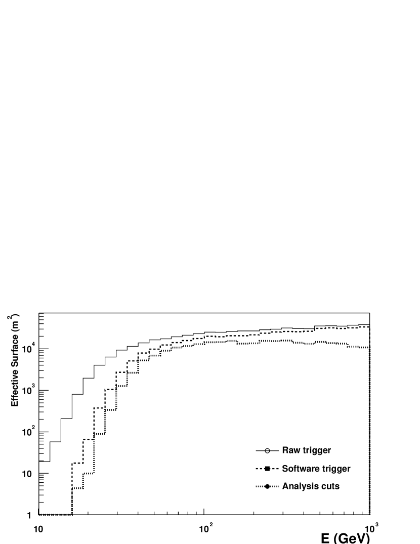
Figure 10: The effective surface area for gamma rays of CELESTE for a trigger threshold of $4.5\mathrm{\ PE}$ per heliostat, in the direction of the Crab at transit. The analysis cuts are $N_{\mathrm{peaks}}\geq 10$ and $\sigma_{\mathrm{grp}}<0.25$.

Fig. 10 shows the effective surface area of CELESTE for gamma rays as a function of the initial photon energy at the raw trigger level, after the software trigger, and after the analysis cuts ($N_{\mathrm{peaks}}\geq 10$ and $\sigma_{\mathrm{grp}}<0.25$), using the KASKADE Monte Carlo. The detector simulation was for 11 km single pointing towards the Crab at transit, with a trigger threshold of $4.5\mathrm{\ PE}$ per heliostat. The curve after cuts can be parametrized as $A(E)=14324(1-e^{(15-E)/8.7})^{5.19}(1-e^{(15-E)/23.9})^{2.38}$ $m^{2}$, with $E$ in GeV. The area is an order of magnitude smaller than for an imaging telescope because convergent viewing restricts the impact parameter at which a gamma shower will be seen by enough heliostats to trigger the experiment.

A valuable partial test of our effective area calculations can be made by using those showers which trigger both CAT and CELESTE. Approximately 20% of the CELESTE events, corresponding to around 30% of CAT events are common and can be identified as such, with a probability better than 99.9%, by their arrival time measured with GPS clocks by the two experiments. During this observing season we have collected 13 hours of common data on the Crab. The standard CAT analysis (le Bohec et al., 1998) when applied to the full data set results in an excess of 1268 gamma events over a background of 3131 hadrons. The same analysis applied only to the common events produces an excess of 418 gammas over a background of 526 hadrons. From these numbers we see that imposing a CELESTE trigger increases the signal to noise ratio in the CAT data sample by a factor of two, although it does not improve the significance of the result as the data sample is smaller.

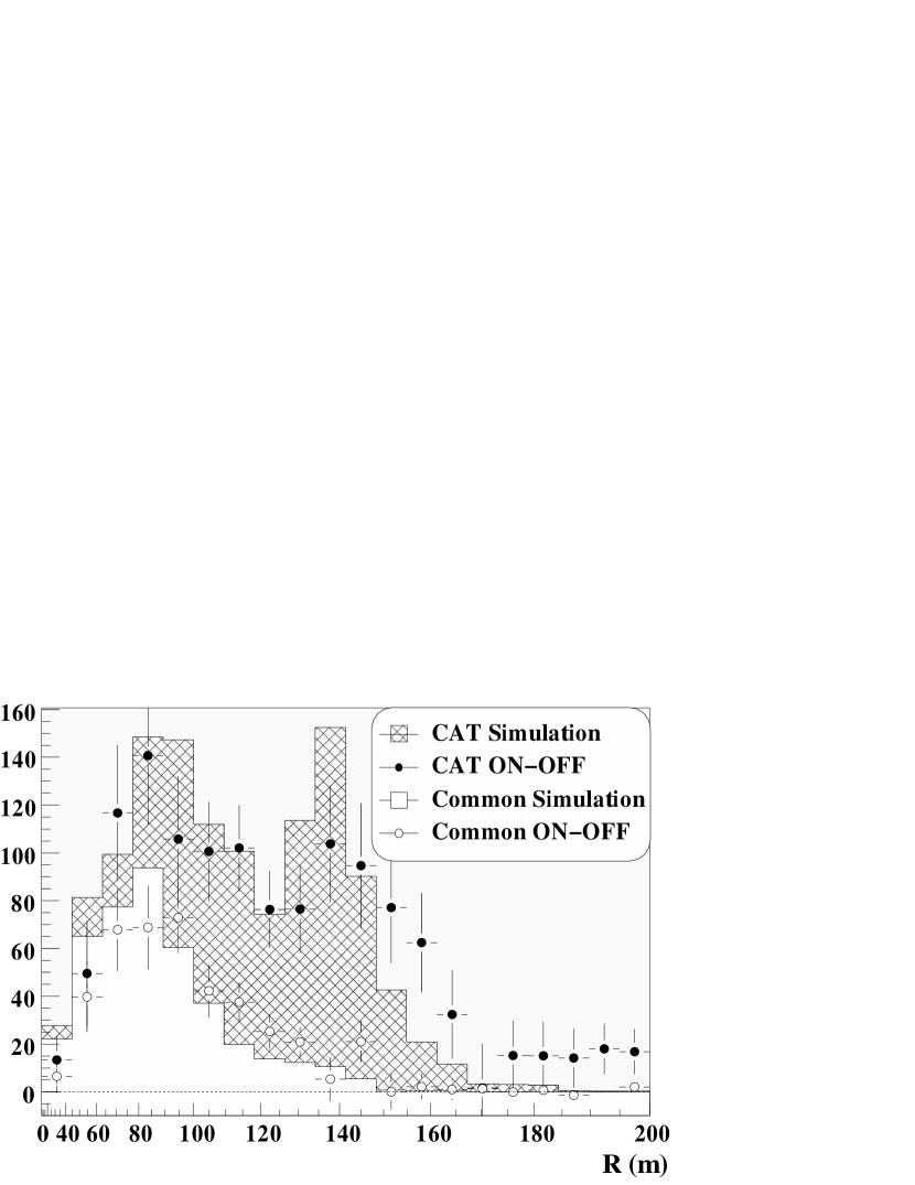
Figure 11: The impact parameter (R) distribution as measured by the CAT experiment for real and simulated gamma rays. The hatched histogram (and filled circles) includes all the CAT events, the clear histogram (and open circles) includes only those events seen by both CAT and CELESTE.

CAT measures the shower impact parameter with better resolution than CELESTE (le Bohec et al., 1998). Fig. 11 shows this reconstructed impact parameter for simulated data, and for the excess events from the common Crab data set. The data are well reproduced by the simulations in terms of both the shape of the distributions and in the predicted fraction of common events. This gives us confidence that the effective surface area for CELESTE, at least in the energy region of the common CAT-CELESTE events, is understood.

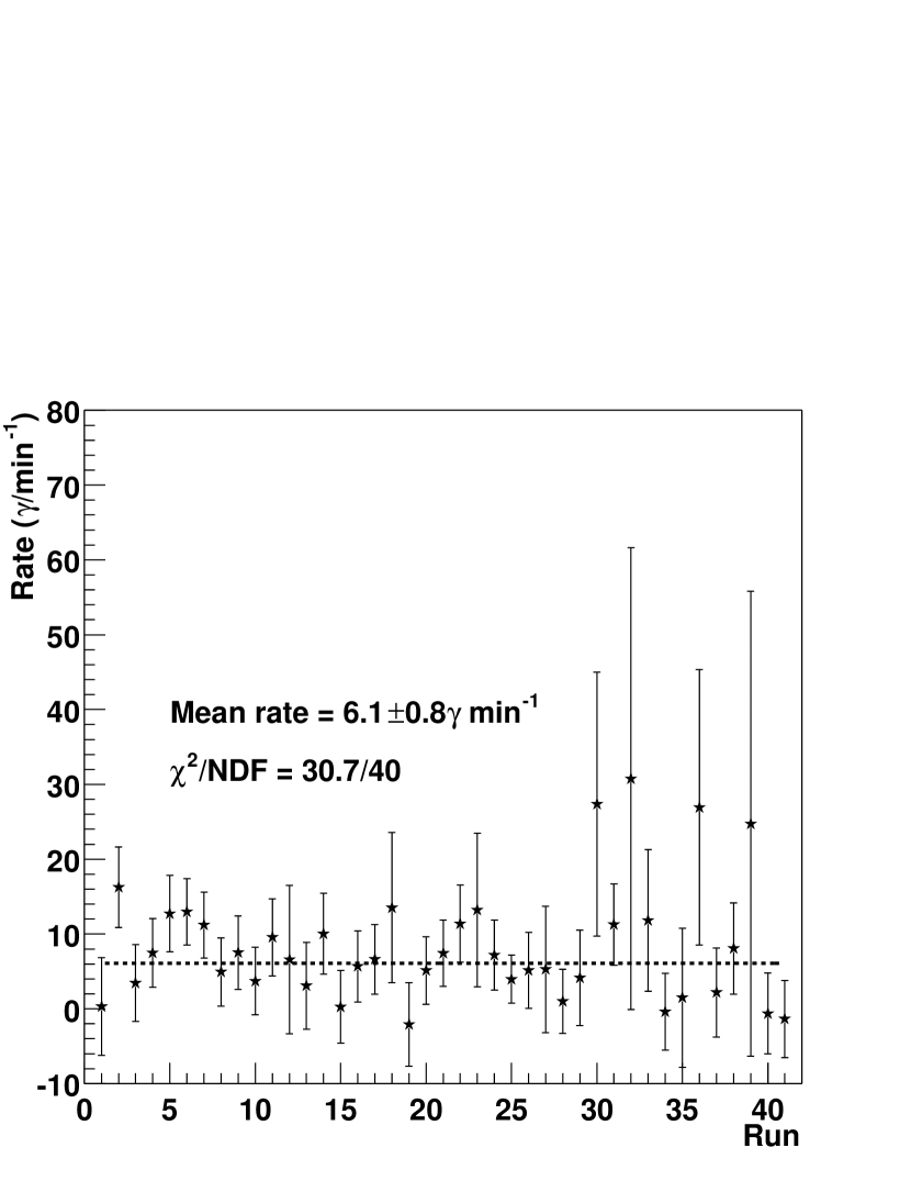
Figure 13: The measured flux for each ON-OFF pair for the 41 Crab runs. The points on the right of the plot have large errors bars as these runs were taken towards the end of the season with the source often far from transit.

The effective area varies with the source position in the sky, as indicated in Fig. 12. Knowing the azimuth angles under which the Crab was observed, we have used the polynomial fit in Fig. 12 to correct our measured gamma ray rate. In addition, for each run we correct for our acquisition dead time of $\sim 20\%$ which is measured during the observations. There is no evidence for time variability in the measured flux of high energy emission from the Crab nebula for gamma ray energies above and below the energy range of CELESTE (de Jager et al., 1996; Vacanti et al., 1991). Fig. 13 shows the rate calculated for each of the 41 ON-OFF pairs, after accounting for the varying gamma ray detection efficiency. A constant fit to these points has a positive mean and a $\chi^{2}$ value of 30.7 for 40 degrees of freedom, as would be expected for a steady signal, which gives us further confidence in the stability of the CELESTE analysis. We obtain the corrected measurement of $6.1\pm 0.8\mathrm{\ \gamma}\mathrm{\ min^{-1}}$ (statistical uncertainty only).

Knowing the effective surface area as a function of energy we can calculate the expected response of CELESTE to a typical spectrum of gamma rays. Fig. 14 shows the energy distributions of simulated events for an input $E^{-2}$ differential gamma ray spectrum, close to the spectral shape for high energy emission from the Crab in the CELESTE energy range (Hillas et al., 1998). A useful definition of the energy threshold for atmospheric Čerenkov detectors is the energy at which the differential gamma ray rate is maximum for a typical source. According to this definition, the energy threshold for CELESTE at the raw trigger level for a source at the position of the Crab at transit is $\sim 30\mathrm{\ GeV}$ . The gamma rays have been simulated with the same distribution of azimuth and zenith angles as the 11 km Crab observations, increasing the energy threshold to $\sim 40\mathrm{\ GeV}$ at the raw trigger stage. As mentioned in the previous section, a software trigger is applied during the analysis to correct for night sky background effects in the data. This increases the energy threshold to a level of $\sim 60\mathrm{\ GeV}$. Further analysis cuts ($N_{\mathrm{peaks}}\geq 10$ and $\sigma_{\mathrm{grp}}<0.25$) reduce the number of gamma rays observed, but do not increase the energy threshold.

The systematic errors on our measurement have two different origins. The uncertainty on the energy scale is due principally to errors in the conversion of the measured signal to a flux of Čerenkov photons, which is a combination of many factors (photon losses through the optical system, PMT quantum efficiencies, electronic calibration errors). We bracket the overall uncertainty arising from the combination of these elements as follows. First, during the CELESTE prototype studies we measured the night sky background in our wavelength range at Themis to be $(2.3\pm 0.4)\times 10^{12}\mathrm{\ photons}\mathrm{\ m}^{-2}\mathrm{\ sr}^{-1}\mathrm{\ s}^{-1}$ (Giebels et al., 1998), in the direction of the Crab at transit (20 degrees south of zenith, towards the populated valley below the site). From this we expect 1 photoelectron per nanosecond per phototube, corresponding to anode currents of $8\mu$A, close to the observed range around $10\mu$A. Studying the FADC pedestal widths used in the padding software also yields values of $\sim 1$ photoelectron per nanosecond per phototube. We further compare currents measured while aligning the heliostats using star scans with predictions from the optical simulation: the measured values are typically 20 % less than expected. Results of studies of the atmospheric extinction using CCD photometry and a LIDAR will be reported in future work but are not included in the present study. Finally, the observed cosmic ray trigger rate is 30% higher than predicted by the Monte Carlo. From these considerations we believe the energy scale uncertainty to be less than $\pm 30$%. The corresponding acceptance curves are $A((1\pm 0.3)E)$, leading to an uncertainty on our threshold. The input spectrum assumed in determining the absolute flux (see discussion below) has little effect on the threshold. For this analysis then, we quote an energy threshold of $60\pm 20\mathrm{\ GeV}$.

The other principal source of systematic error is the uncertainty on our efficiency for detecting gamma rays. As mentioned earlier, there is an energy independent discrepancy of 25% in the effective surface area as calculated using two different shower generation Monte Carlos. Both Monte Carlo’s use the U.S. standard atmosphere. Bernlöhr (2000) recently explored the effects of different atmospheric profiles on the Cherenkov light yield, finding a $\pm 10\%$ variation for 100 GeV gamma rays for midlatitude summer and winter atmospheres, neglecting aerosol variations. We conclude that the uncertainty in the Cherenkov light yield for gamma rays in our energy range is 25%. We also assign a systematic error of 10% to the cut efficiencies deduced from the simulations (Table 3).

5.2 Flux Estimation

At present the event-by-event energy determination in CELESTE is poor. To compare our rate measurement with models and with results from other experiments requires convoluting our detector acceptance, $A(E)$ (see Fig. 10), with an assumed source spectrum. The simplest hypothesis is that of a power law differential flux, $1/E^{\gamma}$. In a $\nu F_{\nu}$ representation (or, equivalently, $E^{2}{dN\over dE}$) the CELESTE energy range corresponds to the top of the parabola-like spectral shape attributed to inverse Compton production of gamma rays in the nebula (Hillas et al., 1998), and $\gamma=2$ is a good approximation. It yields an integral result for CELESTE of $I(E>60\mathrm{\ GeV})=5.5\times 10^{-6}\mathrm{\ photons}\mathrm{\ m^{-2}}\mathrm{\ s^{-1}}$. STACEE used this approach, with $\gamma=2.4$ (Oser et al., 2001).

A more realistic hypothesis recognizes that the spectrum deviates from a pure power law. We use a parabola-like spectral shape of the form

$$E^{2}{dN\over dE}=kE^{\alpha+\beta\log_{10}E}.$$

Above $500\mathrm{\ GeV}$ we use the values of $k,\alpha$, and $\beta$ taken from CAT (Masterson et al., 2001). Below $500\mathrm{\ GeV}$ we let $\beta$ be a free parameter, but require continuity at 500 GeV. We determine $\beta_{C}$ such that the convolution with $A(E)$ yields our measured rate and thus obtain an integral flux of $I(E>60\mathrm{\ GeV})=6.2\times 10^{-6}\mathrm{\ photons}\mathrm{\ m^{-2}}\mathrm{\ s^{-1}}$. We further vary $\beta$ and determine that the range of ($3.9$ to $11.5)\times 10^{-6}\mathrm{\ photons}\mathrm{\ m^{-2}}\mathrm{\ s^{-1}}$ is consistent with the rate and acceptance uncertainties, including that of the energy scale. Repeating the process using the Whipple (Hillas et al., 1998), or HEGRA (Aharonian et al., 2000) spectra gives very nearly the same results. We thus determine our flux to be

$$I(E>60\mathrm{\ GeV})=6.2^{+5.3}_{-2.3}\times 10^{-6}\mathrm{\ photons}\mathrm{\ m^{-2}}\mathrm{\ s^{-1}}.$$

We applied this procedure above 190 GeV to compare with STACEE and obtain $I(E>190\mathrm{\ GeV})=1.8\times 10^{-6}\mathrm{\ photons}\mathrm{\ m^{-2}}\mathrm{\ s^{-1}}$ in agreement with their result of $I(E>190\mathrm{\ GeV})=2.2\pm 0.6\pm 0.2\times 10^{-6}\mathrm{\ photons}\mathrm{\ m^{-2}}\mathrm{\ s^{-1}}$.

To represent this integral measurement on a differential plot, we use $\beta_{C}$ to calculate $E^{2}{dN\over dE}$ at our energy threshold. This is shown as a triangle in Fig. 15. As above, the error bar is obtained by finding the range of $\beta$ that accomodates the uncertainties on our measurement. The value shown is $3.1^{+6.3}_{-1.8}\times 10^{-4}\mathrm{\ GeV}\mathrm{\ m}^{-2}\mathrm{\ s}^{-1}$. Fig. 15 also shows the imager measurements, as well as the envelope defined by varying the imager fit parameters $k,\alpha$, and $\beta$ by one standard deviation around their central values. Our measurement favors the lower part of the range allowed by the imagers and is compatible with the results from EGRET.

6 Periodicity Search

One of the primary goals of the CELESTE experiment is to investigate the periodic emission from gamma ray pulsars in the cutoff region below 100$\mathrm{\ GeV}$. The CELESTE data include the arrival time of each event measured to a precision of $<1\mu$s using a time-frequency processor slaved to a Global Positioning System (GPS) clock which provides synchronisation every second. This timing information has been used to search for evidence of periodicity in our Crab data.

In order to verify our periodic analysis procedure we have made observations of the optical emission from the Crab pulsar using the CELESTE heliostats. Given the optical flux from the Crab pulsar (Percival et al., 1993), we expect a flux of $\sim 1\times 10^{4}\mathrm{\ PE}\mathrm{\ s^{-1}}\mathrm{\ heliostat^{-1}}$ over a night sky background of typically $\sim 1\times 10^{9}\mathrm{\ PE}\mathrm{\ s^{-1}}\mathrm{\ heliostat^{-1}}$.

In standard operation, the PMT anode currents for all forty heliostats are converted to a buffered voltage which is digitized and stored with the data stream. The current-to-voltage conversion integrates the signal over $<1~{}\mathrm{\ ms}$. For the optical pulsar study, three of these current outputs were AC-coupled, in order to subtract the steady component due to the night sky background and the nebula, and sent to a 16-bit ADC card readout by a PC at a frequency of $2000\mathrm{\ Hz}$. A GPS time reference was obtained for the optical data by sending the same pulse every $10\mathrm{\ s}$ as a trigger to CELESTE and as data to the ADC card. We then tracked the Crab pulsar and recorded the current fluctuations during 30 minutes. The synchronised times were converted to the solar system barycenter frame using the JPL DE200 ephemeris (Standish, 1982). Fig. 16 shows the phase histogram using the frequency ephemerides obtained by (Lyne et al., 2000). The double-peaked signal from the pulsar is clearly visible. We use the same code to calculate the phase of the air shower events.

From the EGRET pulsar detections, the TeV upper limits, and the model predictions it is clear that the search for pulsed gamma ray emission requires as low an energy threshold as possible. To date we have no evidence of a pulsed signal. We present the pulsar search using the same analysis as used to measure the steady emission flux, that is, applying the software trigger, $N_{\mathrm{peaks}}\geq 10$ and $\sigma_{\mathrm{grp}}<0.25$. Although this raises our energy threshold, we take this cautious approach because the efficiency is better understood.

The light curves of both the ON source data and the OFF source data remaining after cuts for the $12.1\mathrm{\ hour}$ Crab data set of Table 1 are shown in Fig. 17. Table 5 summarises the contents of the plots as well as the results of the H-test (de Jager, 1994). The distributions are statistically flat. In order to calculate upper limits for the pulsed emission we assume that the pulse profile is the same as that seen by EGRET at lower energies with emission concentrated in a main pulse in the phase range 0.94-0.04 and a secondary pulse in the range 0.32-0.43 (Fierro et al., 1998). We use the method of Helene to determine an upper limit of $<N_{p}=332$ pulsed events at the 99% confidence level (Helene et al., 1998). This corresponds to 12% of the observed steady signal.

We include the detector acceptance as follows. We take the double power law fit of the total spectrum measured by EGRET (Fierro et al., 1998), and attenuate the sum with an exponential cutoff,

$${dN\over dE}|_{att}=[0.7(E/100)^{-4.89}+2.3(E/100)^{-2.05}]e^{-E/E_{0}},$$

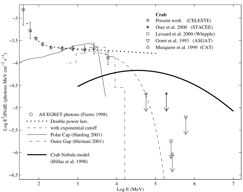
Figure 18: Pulsed photon spectrum of the Crab pulsar (after Lessard et al. (2000)). The EGRET data points are for all phase values, with the double power-law fit from Fierro et al. (1998). The fit is attenuated by an exponential with cutoff energy $E_{0}=26\mathrm{\ GeV}$ derived from the CELESTE upper limit (dashed curve). The CELESTE mean energy is shown by the open star on the curve. The thin solid line is the polar cap model applied to the Crab (A.K. Harding 2001, private communication). The dotted line is the outer gap model corresponding to the dashed line in Figure 4 of Hirotani & Shibata (2001) (for the case $\mathrm{j}_{gap}=0.01,~{}\mathrm{j}_{1}=0.25,~{}\mathrm{j}_{2}=0$: see paper for details). The thick solid line shows the model of unpulsed GeV-TeV emission from the Crab Nebula (Hillas et al., 1998)

in units of $10^{-8}$ photons cm^-2s^-1MeV^-1. We convolute this spectrum with the acceptance after cuts shown in Fig. 14, and find that for $E_{0}=20$ GeV we would expect $N_{p}$ events. Including the 30% uncertainty in the energy determination degrades this value to $E_{0}=26$ GeV. Fig. 18 shows ${dN\over dE}|_{att}$, where we have placed a point at the energy threshold obtained for our steady signal to guide the eye. We note that our limit is not directly comparable to that obtained by the STACEE (Oser et al., 2001) group since they used the larger acceptance corresponding to their measured steady spectrum for comparison with the prediction of TeV pulsed emission. Our hypothesis of an attenuated EGRET spectrum restricts our acceptance to the low energy range of Fig.14, yet our upper limit still provides the most constraining measurement so far on the position of the cutoff point. In the future, improved trigger electronics and observing and analysis strategies optimized for pulsar observations should allow us to increase our acceptance at low energy.

7 Discussion

The radiation from the Crab nebula is dominated by non-thermal emission which is believed to be generated by synchrotron radiation from highly relativistic electrons with energies up to $\sim 10^{15}\mathrm{\ eV}$.

The electrons are accelerated at the shock front where a relativistic wind of charged particles emerging from the pulsar meets the surrounding nebula (Rees & Gunn, 1974; Kennel & Coroniti, 1984). Recent high resolution X-ray observations by the Chandra observatory have shown an inner ring of X-ray emission which may correspond to the position of this shock (Weisskopf, et al., 1999). Aharonian & Atoyan (1995) and Atoyan & Aharonian (1996) have described the electrons in terms of two populations of different energies. The first, generated over the whole lifetime of the nebula and covering energies up to $\sim 100\mathrm{\ GeV}$, produces synchrotron radiation from radio wavelengths to the far infra-red while the second, more recently accelerated population, with energies $>10^{12}\mathrm{\ eV}$ produces synchrotron emission from the infra-red up to $\sim$1 GeV.

It was first suggested by Gould (1965) (also Rieke & Weekes (1969) and Grindlay & Hoffman (1971)) that the synchrotron self-Compton mechanism could give rise to radiation from the Crab above $1\mathrm{\ GeV}$. This process, in which inverse Compton scattering of the synchrotron photons by the relativistic electrons boosts the photons up to much higher energies, has been modelled by various workers, most recently de Jager & Harding (1992), Atoyan & Aharonian (1996) and Hillas et al. (1998). While the synchrotron photons are the most important component, photons due to infra-red emission from dust and to the microwave background will also be upscattered and contribute significantly to the high energy emission.

Fig. 15 shows the result of this work along with the measurements from EGRET and three atmospheric Cherenkov imaging telescopes. The shape of the inverse Compton spectrum is relatively insensitive to the model parameters, but the absolute flux depends strongly upon the magnetic field strength in the emitting region, which in turn depends upon $\sigma$, the ratio of the magnetic field strength to particle energy density in the pulsar wind. Atoyan & Aharonian (1996) have proposed that an additional component due to Bremsstrahlung radiation from the relativistic electrons in dense filaments of nebular gas may provide an increased flux in the $1-100\mathrm{\ GeV}$ range, which could account for a possible discrepancy between the models and the EGRET points around $1\mathrm{\ GeV}$. The uncertainties are still large but the CELESTE measurement does not seem to point towards such an effect. The calibration of such a complex instrument as CELESTE is a large project in itself. Our measurement errors are currently dominated by systematic effects which should decrease as this work proceeds, the most important being to improve our determination of the energy scale.

The Crab pulsar is a source of 33$\mathrm{\ ms}$ pulsed radiation from radio wavelengths to GeV gamma ray energies. Periodic emission is observed by EGRET up to energies of $10\mathrm{\ GeV}$ (Ramanamurthy et al., 1995). Despite early claims (Gibson et al., 1982; Bhat et al., 1986; Dowthwaite et al., 1984), no pulsed emission has been detected by the present generation of ground based atmospheric Čerenkov experiments. The previous best upper limits are at $250\mathrm{\ GeV}$, from the Whipple (Lessard et al., 2000) and CAT (Musquere et al., 1999) groups, and the limit at $190\mathrm{\ GeV}$ by STACEE (Oser et al., 2001).

Two general classes of models have been proposed to describe the pulsed gamma ray emission from the high energy pulsars observed by EGRET. In the polar cap models (Daugherty & Harding, 1982, 1996; Sturner et al., 1995) electrons accelerated from the neutron star surface at the magnetic pole emit by curvature radiation or magnetic inverse Compton scattering, triggering photon-pair cascades in the pulsar magnetosphere from which the observed radiation emerges. Outer gap (Cheng, Ho & Ruderman, 1986; Romani & Yadigaroglu, 1995) models place the emission region in the outer magnetosphere where electrons are accelerated across charge depleted regions near the light cylinder. Both models predict a cutoff in the pulsed emission below $100\mathrm{\ GeV}$, and the exact position for the cutoff can be used to discriminate between them.

Hirotani & Shibata (2001) treat the electrodynamics of the outer gap from first principles. The free parameter in their model is the current density at the gap boundaries, which in turn depends on the distance of the gap from the light cylinder. Our upper limit excludes the hypothesis that the current density vanishes at the gap surface, since the model predicts a gamma ray flux extending to 60 GeV in that case. Fig. 18 includes the prediction of their model for the case of a small current density at the inner boundary, and a null current at the outer boundary. Fig. 18 also shows the predictions of a polar cap model, along with the EGRET measurements and higher energy upper limits. The CELESTE upper limit constrains the high energy emission more strongly than the previous Whipple measurement, but increased sensitivity at lower energy is still needed to favor a particular model for the emission processes.

8 Conclusions

We have presented the first detection by the atmospheric Čerenkov technique of a gamma ray source, the Crab nebula, at energies below 100$\mathrm{\ GeV}$ using the CELESTE experiment. The measured flux is compatible with most emission models. No periodic signal has been detected but our upper limit allows us to constrain further the cutoff point for emission from the pulsar. As our uncertainties decrease we will be able to determine the energy range in which the nebula and pulsar contributions are comparable.

The data reported on in this paper were collected during the first observation season with a fully operational 40 heliostat array. In single pointing mode we now have a sensitivity to the Crab of $2.1\sigma/\sqrt{hour}$. A smaller dataset obtained with heliostat double pointing appears to confirm Monte Carlo predictions of improved sensitivity, yielding $3.4\sigma/\sqrt{hour}$, although more data is required for confirmation. It seems likely that a posteriori optimization of our hadron rejection cuts, along with the development of new analysis techniques, will enable us to improve our sensitivity in the future. CELESTE is currently being upgraded by the addition of another 13 heliostats, bringing the total to 53, allowing greater flexibility in pointing strategies.

Figure 5: Test of the software trigger. The Crab data set is divided into two halves as described in the text. The upper plots show the ON-OFF distribution of total charge for the raw data after software padding. The lower plots show the same after application of the software trigger.

Figure 12: The simulated gamma ray detection efficiency for CELESTE Crab observations as a function of time of the observation relative to Crab transit. The efficiency is normalized to the raw trigger simulated gamma ray rate at the Crab transit. The simulations were made only for azimuth directions before Crab transit - we rely on the symmetry of the heliostat field to extrapolate to after transit. The errors are statistical only. The analysis cuts are after the software trigger, with $N_{\mathrm{peaks}}\geq 10$ and $\sigma_{\mathrm{grp}}<0.25$.

Figure 15: The very high energy spectrum of the Crab. The spectra measured by three Cherenkov imaging telescopes are shown by the thin curves (Hillas et al., 1998; Aharonian et al., 2000; Masterson et al., 2001). Varying the imager fit parameters by one standard deviation gives the range bound by the solid thick curves. The thick dashed curves extend the envelope to lower energies. The flux shown for CELESTE (triangle) corresponds to the spectral shape which, when convoluted with the detector acceptance, yields the observed gamma ray rate (see text). The point is placed at the nominal energy threshold, with the energy scale uncertainties included in the error in the flux determination. Also shown is the spectrum of all photons detected by EGRET (open dots) (Fierro et al., 1998), and the EGRET data attributed to the nebula (black dots) (de Jager et al., 1996).

Figure 16: Phase histogram for the optical Crab data.

Figure 17: Phase Histograms for the ON source and OFF source CELESTE 11km Crab observations. Both are statistically flat.

Table 1: Crab observations for the 1999/2000 observing season.

Pointing Altitude	Number	Number	ON Source Duration	Dates
(km)	of Pairs	Used	(hours)
11	75	41	12.1	11/99 - 03/00
11-25	12	9	2.2	01/00 - 02/00

Table 2: The number of events remaining at each stage of the analysis for the 11km single pointing Crab data set.

Cut	Number	Number	Difference	Significance	Signal/	$\gamma$ rate
	ON	OFF		($\sigma$)	Background	($\mathrm{\ min^{-1}}$)
Raw Trig.	$894\,494$	$888\,725$	$5\,769$	$4.3$	$0.6\%$	$\cdots$
Software Trig.	$474\,823$	$469\,312$	$5\,511$	$5.7$	$1.2\%$	$7.6$
$N_{\mathrm{peaks}}\geq 10$	$434\,368$	$429\,242$	$5\,126$	$5.5$	$1.2\%$	$7.1$
$\sigma_{\mathrm{grp}}<0.25$	$67\,022$	$64\,295$	$2\,727$	$7.5$	$4.2\%$	$3.8$
$\theta\leq 7\mathrm{\ mrad}$	$41\,442$	$39\,481$	$1\,961$	$6.9$	$5.0\%$	$2.7$

Table 3: Cut efficiencies calculated from the real Crab data and from simulated gamma rays (statistical errors only). Shown are the incremental effects of each successive cut (top section), as well as the cumulative efficiencies (bottom section). The last line shows the cuts used in the flux determination.

		Real Data		Simulation
Cut		OFF	ON-OFF	$\gamma$
Software Trigger (S.T.)		$52.8\pm 0.1\%$	$\cdots$	$59.4\pm 0.3\%$
$N_{\mathrm{peaks}}\geq 10$		$91.5\pm 0.2\%$	$93\pm 24\%$	$90.2\pm 0.6\%$
$\sigma_{\mathrm{grp}}<0.25$		$15.0\pm 0.1\%$	$53\pm 12\%$	$61.2\pm 0.5\%$
$\theta\leq 7\mathrm{\ mrad}$		$61.4\pm 0.4\%$	$72\pm 14\%$	$85.2\pm 0.7\%$
All cuts		$4.44\pm 0.02\%$	$\cdots$	$28.0\pm 0.2\%$
All cuts, after S.T.		$8.41\pm 0.04\%$	$36\pm 8\%$	$47.1\pm 0.4\%$
$N_{\mathrm{peaks}}\geq 10$, $\sigma_{\mathrm{grp}}<0.25$, after S.T.		$13.7\pm 0.1\%$	$49\pm 17\%$	$55.2\pm 0.6\%$

Table 4: The number of events remaining at each stage of the analysis for the $11\mathrm{\ km}$ and $25\mathrm{\ km}$ double pointing Crab data set.

Cut	Number	Number	Difference	Significance	Signal/	$\gamma$ rate
	ON	OFF		($\sigma$)	Background	($\mathrm{\ min^{-1}}$)
Raw Trig.	$157\,129$	$155\,365$	$1\,764$	$3.2$	$1.1\%$	$\cdots$
Software Trig.	$79\,685$	$78\,381$	$1\,304$	$3.3$	$1.7\%$	$10.0$
$N_{\mathrm{peaks}}\geq 10$	$75\,193$	$73\,900$	$1\,293$	$3.3$	$1.7\%$	$9.9$
$\sigma_{\mathrm{grp}}<0.25$	$9\,174$	$8\,523$	$651$	$4.9$	$7.6\%$	$5.0$
$\theta\leq 7\mathrm{\ mrad}$	$5\,733$	$5\,209$	$524$	$5.0$	$10.1\%$	$4.0$

Table 5: .

Total number of ON events	67022
Total number of OFF events	64295
Pulsed phase fraction	0.21
Number of ON events in expected phase windows	14062
Number of ON events outside expected phase windows	52960
Significance for the pulsed phase domain	$-0.1\sigma$
Value of the H-test for ON source events	2.60
Value of the H-test for OFF source events	1.17
Upper limit at the 99% confidence level for H-test	$<31\%$
Upper limit at the 99% confidence level using Helene method	$<12\%$

References

- Aharonian & Atoyan (1995) Aharonian, F.A. & Atoyan, A.M., 1995, Astropart Phys, 3, 275
- Aharonian et al. (1999) Aharonian, F., et al., 1999, A&A, 346, 913
- Aharonian et al. (2000) Aharonian, F.A., et al., 2000, ApJ, 539, 317
- Arqueros et al. (2001) Arqueros, F., et al., 2001, Astropart. Phys. submitted
- Atoyan & Aharonian (1996) Atoyan, A.M. & Aharonian, F.A., 1996, MNRAS, 278, 525
- Baillon et al. (1993) Baillon, P., et al., 1993, Astropart. Phys., 1, 341
- Barrau et al. (1998) Barrau, A., et al., 1998, Nucl. Instrum. Meth., A416, 278
- Bernlöhr (2000) Bernlöhr, K. 2000, Astropart. Phys. 12, 255.
- Bhat et al. (1986) Bhat, P.N., et al., 1986, Nature, 319, 127
- le Bohec et al. (1998) le Bohec, S., et al., 1998, Nucl. Instrum. Methods A, 416, 425
- Bradbury et al. (1999) Bradbury, S.M., et al., 1999, in The 26th International Cosmic Ray Conference, ed. D. Kieda, M. Salomon, B. Dingus (Salt Lake City), 5, 280
- Cawley (1993) Cawley, M.F., 1993, in Towards a Major Atmospheric Čerenkov Detector - II, ed. R.C. Lamb (Calgary), p176
- Cheng, Ho & Ruderman (1986) Cheng, K.S., Ho, C. & Ruderman, M., 1986, ApJ, 300, 500
- Covault et al. (2001) Covault, C. et al. in The 27th International Cosmic Ray Conference, (Hamburg, 2001) in press.
- Daugherty & Harding (1982) Daugherty, J.K. & Harding, A.K., 1982, ApJ, 252, 357
- Daugherty & Harding (1996) Daugherty, J.K. & Harding, A.K., 1996, ApJ, 458, 278
- Dermer & Schlickeiser (1993) Dermer, C. D. & Schlickeiser, R., 1993, ApJ, 416, 458
- Dowthwaite et al. (1984) Dowthwaite, J.C., et al., 1984, ApJ, 286, L35
- Fierro et al. (1998) Fierro, J.M.. et al., 1998, ApJ, 494, 734
- Ghisellini & Maraschi (1996) Ghisellini, G. & Maraschi, L., 1996, in ASP Conf. Ser. 110, Blazar Continuum Variability, ed. H. R. Miller, J. R. Webb, & J. C. Noble (San Francisco: ASP), 436
- Gibson et al. (1982) Gibson, A.I., et al., 1982, Nature, 296, 833
- Giebels et al. (1998) Giebels, B., et al., 1998, Nucl. Instr. Meth. A 412, 329, with additional details in the doctoral thesis available at http://infodan.in2p3.fr/themis/CELESTE/PUB/giebels.ps.gz
- Goret et al. (1993) Goret, P., et al., 1993, A&A, 270, 401
- Gould (1965) Gould, R.J., 1965, Phys.Rev.Lett., 15, 577
- Grindlay & Hoffman (1971) Grindlay, J.E. & Hoffman, J.A., 1971, Ap. Letters, 8, L209
- Heck et al. (1998) Heck, D., et al., 1998, Report FZKAS 6019, Forschungszentrum Karlsruhe
- Helene et al. (1998) Helene, O., 1983, Nucl. Instrum. Methods, 212, 319
- Herault (2000) Herault, N., 2000, Reconstruction des paramètres des gerbes de gamma et contribution à l’analyse des données dans l’expérience CELESTE, Thèse de Doctorat, Université Louis Pasteur de Strasbourg, http://www.lal.in2p3.fr/presentation/bibliotheque/publications/Theses00.html
- Hillas et al. (1998) Hillas, A.M. et al., 1998, ApJ, 503, 744
- Hirotani & Shibata (2000) Hirotani, K. & Shibata, S., 2000, preprint (astro-ph/0011488)
- Hirotani & Shibata (2001) Hirotani, K. & Shibata, S., 2001, preprint (astro-ph/0101498)
- Holder et al. (2000) Holder, J., et al., 2000 in Heidelberg Gamma Ray Symposium, ed. F.A. Aharonian & H. Voelk, 635
- de Jager & Harding (1992) de Jager, O.C. & Harding, A.K., 1992, ApJ, 396, 161
- de Jager (1994) de Jager, O.C., 1994, ApJ, 436, 239
- de Jager et al. (1996) de Jager, O.C., et al., 1996, ApJ, 457, 253
- Kennel & Coroniti (1984) Kennel, C.F. & Coroniti, F.V., 1984, ApJ, 283, 694 and 710
- Kertzmann & Sembroski (1994) Kertzmann, M.P. & Sembroski, 1994, Nucl. Instrum. Methods A, 343, 629
- Kohnle et al. (1999) Kohnle, A., et al., 1999, in The 26th International Cosmic Ray Conference, ed. D. Kieda, M. Salomon & B. Dingus (Salt Lake City), 5, 239
- Lessard et al. (2000) Lessard, R.W., et al., 2000, ApJ, 531, 942
- Lyne et al. (2000) Lyne, A.G., Pritchard, R.S. & Roberts, M. at http://www.jb.man/ac.uk/ pulsar/crab.html
- Marcowith et al. (1995) Marcowith, A., Henri, G. & Pelletier, G. 1995, MNRAS, 277, 681
- Masterson et al. (2001) Masterson, C., et al., in proc. Gamma-2001 conference (Baltimore), (in press)
- Martinez et al. (1999) Martinez, M., et al., 1999, in The 26th International Cosmic Ray Conference, ed. D. Kieda, M. Salomon, B. Dingus (Salt Lake City), 5, 219
- Musquere et al. (1999) Musquere, A., et al., 1999, in The 26th International Cosmic Ray Conference, ed. D. Kieda, M. Salomon, B. Dingus (Salt Lake City), 3, 460
- de Naurois (2000) de Naurois, M., 2000, Reconversion d’une centrale solaire pour l’astronomie . Première observation de la Nébuleuse du Crabe et du Blazar Markarian 421 entre et , Thèse de Doctorat, Université Paris VI, http://polywww.in2p3.fr/celeste/these/These.html
- Oser et al. (2001) Oser, S., et al., 2001, ApJ, 547, 949
- Punch et al. (1991) Punch, M., et al., 1992, Nature 358, 477.
- Percival et al. (1993) Percival, J.W. et al., 1993, ApJ, 407, 276
- Piron et al. (2000) Piron, F., 2000, Etude des propriétés spectrales et de la variabilité de l’émission Gamma supérieure à 250 GeV des noyaux actifs de galaxies de type blazar observés dans le cadre de l’expérience CAT, Thèse de Doctorat, Université Paris XI, http://lpnp90.in2p3.fr/ cat/Papers/these_piron.ps.gz
- Ramanamurthy et al. (1995) Ramanamurthy, P.V., et al., 1995, ApJ, 450, 791
- Rees & Gunn (1974) Rees, M.J. & Gunn, J.E., 1974, MNRAS, 167, 1
- Reposeur et al. (2001) Reposeur, T. et al., to be submitted to Nucl. Instr. Meth. (2001)
- Rieke & Weekes (1969) Rieke, G.H. & Weekes, T.C., 1969, ApJ, 155, 429
- Romani & Yadigaroglu (1995) Romani, R.W. & Yadigaroglu, I-A., 1995, ApJ, 438, 314
- Romani (1996) Romani, R.W., 1996, ApJ, 470, 469
-
Smith et al. (1996)
Smith, D.A., et al., CELESTE
experimental proposal,
http://polywww.in2p3.fr/celeste/public/cxp.ps.gz - Standish (1982) Standish, E.M., Jr., 1982, A&A, 114, 297
- Sturner et al. (1995) Sturner, S.J., Dermer, C. D. & Michel, F.C., 1995, ApJ, 445, 736
- Vacanti et al. (1991) Vacanti, G. et al., 1991, ApJ, 377, 467
- Weekes et al. (1989) Weekes, T. C. et al., 1989, ApJ, 342, 379
- Weisskopf, et al. (1999) Weisskopf, M.C., et al., 2000, ApJ 536, L81.