Discrete Dynamical Classes For Galaxy Discs
and the implication of a second generation of
Tully-Fisher Methods

In Roscoe 1999a , it was described how the modelling of a small sample of optical rotation curves (ORCs) given by Rubin et al Rubin (1980) with the power-law $V_{rot}=AR^{\alpha}$, where where the parameters $(A,\alpha)$ vary between galaxies, raised the hypothesis that the parameter $A$ (considered in the form $\ln A$) had a preference for certain discrete values. This specific hypothesis was tested in that paper against a sample of 900 spiral galaxy rotation curves measured by Mathewson et al Mathewson1992 (1992), but folded by Persic & Salucci Persic1995 (1995), and was confirmed on this large sample with a conservatively estimated upper bound probability of $10^{-7}$ against it being a chance effect. In this paper, we begin by reviewing the earlier work, and then describe the analyses of three additional samples; the first of these, of 1200+ Southern sky ORCs, was published by Mathewson & Ford Mathewson1996 (1996), the second, of 497 Northern sky ORCs, is a composite sample provided by kind permission of Giovanelli & Haynes published in the sequence of papers Dale et al Dale1997 (1997), Dale1998 (1998), Dale1999 (1999) and Dale & Uson Dale2000 (2000), whilst the third, of 305 Northern sky ORCs, was published by Courteau Courteau (1997). These analyses provide overwhelmingly compelling confirmation of what was already a powerful result. Apart from other considerations, the results lead directly to what can be described as a ‘second generation of Tully-Fisher methods.’ We give a brief discussion of the further implications of the result.

1 Introduction

This paper describes the analyses of four large optical rotation curve samples to show how the hypothesis that ‘spiral galaxies are constrained to occupy discrete dynamical classes’ is supported by the data as a statistical certainty. At a practical level, the result has considerable immediate implications for the absolute determination of zero points for classical Tully-Fisher methods and, in the wider context of the overall analysis, provides a class of second generation Tully-Fisher methods in which absolute Tully-Fisher calibrations and linewidth determinations can, in principle, be simultaneously determined on any given sample of ORCs. At a deeper level, the basic result appears to have implications for our understanding of galaxy evolution. The result is so unexpected, that a short review of already published material (Roscoe 1999a ) is likely to be useful to the present reader.

Arguments based on certain symmetry considerations - the nature of which are not immediately relevant here - led us to consider the possibility that the segments of optical rotation curves which occupy disc regions (given an operational definition later in this text) might be reasonably described - in an overall statistical sense - by power laws in the form $V_{rot}\,=\,AR^{\alpha}$, with the parameters $A$ and $\alpha$ being determined empirically for each galaxy in turn. As a means of gaining familiarity with this idea, we considered the small sample of 21 ORCs published by Rubin et al Rubin (1980) from this point of view. Of this sample of 21 ORCs, only twelve manifested reasonably monotonic behaviour and so were selected on these grounds alone as reasonable candidates for a power law analysis. Subsequently, a linear regression of the model $\ln V_{rot}\,=\,\ln A\,+\,\alpha\ln R$ onto each of the twelve ORCs provided twelve sets of parameter-pairs $(\alpha,\,\ln A)$. The first clear result of this mini-analysis was that $\alpha$ and $\ln A$ appeared to be very strongly correlated - and this particular aspect has now been analysed in detail using Persic & Salucci’s Persic1995 (1995) folding solution for 900 ORCs from the Mathewson et al Mathewson1992 (1992) sample (Roscoe 1999b ).

However, as reference to table 1 shows (the entries of which have been rounded to the nearest decimal), a curious numerical coincidence arose - specifically, that every one of the twelve $\ln A$ values lay between $\pm 0.15$ of an integer or half-integer value - a coincidence that has odds around 1:500 of being a chance occurrence ( a-posteriori probabilities !). Of course, the integer/half-integer values themselves can be of no possible significance since, if Rubin et al Rubin (1980) had estimated distance scales using a value of $H$ significantly different from the $50$km/sec/Mpc they actually used, then a completely different set of $\ln A$ values would have resulted. So, the coincidence was simply that of regularity in spacing which would probably have not been noticed with, say, $H\,=\,70$km/sec/Mpc. Anyway, curiosity provided a sufficient motivation to consider the matter further, using the Persic & Salucci Persic1995 (1995) sample of 900 folded ORCs.

Table 1: Twelve Rubin, Ford & Thonnard Rubin (1980) spirals

Galaxy	$\ln A$	Galaxy	$\ln A$
N3672	3.6	U3691	3.6
N3495	4.0	N4605	4.0
I0467	4.1	N0701	4.1
N1035	4.1	N4062	4.5
N2742	4.5	N4682	4.5
N7541	4.6	N4321	4.9

Table 2: $\ln A$ data

RFT	Pred value	Actual value
scale	with MFB	MFB
	scale	scale
3.5	3.81	3.85
4.0	4.22	4.24
4.5	4.63	4.72
5.0	5.04	5.06

This sample had its distance-scaling determined by a Tully-Fisher relationship calibrated by Mathewson et al Mathewson1992 (1992) against Fornax using $H\,=\,85$km/sec/Mpc, so that the integer/half-integer hypothesis for $\ln A$ is not appropriate. However, a simple analysis (described in Appendix B of Roscoe 1999a , and relying on the investigation of the $(\alpha,\,\ln A)$ correlation given in Roscoe 1999b ) reveals the relation

$$\ln A_{MFB}\,\approx\,0.82\,\ln A_{RFT}\,+\,0.94$$

where $A_{MFB}$ denotes the value of $A$ determined using the Mathewson et al Mathewson1992 (1992) scaling, whilst $A_{RFT}$ denotes its value determined using the Rubin et al Rubin (1980) scaling. Using this latter relation, the integer/half-integer values of $\ln A$ in the Rubin et al Rubin (1980) scaling transform into their corresponding value in the Mathewson et al Mathewson1992 (1992) scaling according to the first two columns of table 2.

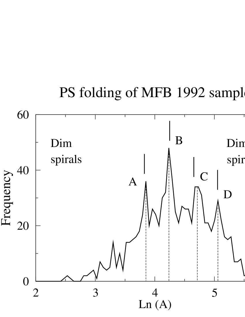
Figure 1: $\ln A$ distribution for the Mathewson et al Mathewson1992 (1992) sample with Persic & Salucci folding. Vertical dotted lines indicate actual peak centres. Vertical solid bars indicate predicted peak centres from the Rubin et al Rubin (1980) sample. Bin width = 0.055.

The actual $\ln A$ distribution of the 900 ORCs of the Mathewson et al Mathewson1992 (1992) sample folded by Persic & Salucci Persic1995 (1995) is given in figure 1. The vertical solid bars indicate the predicted positions of the peaks, based on our analysis of the Rubin data, as in the second column of table 2, whilst the vertical dotted lines indicate actual peak centres, as in the third column of table 2. The correspondence between the peak positions, predicted on the basis of the twelve Rubin et al Rubin (1980) galaxies of table 1, and the actual peak positions is clearly remarkable. A crude, but extremely conservative, upper bound estimate of the probability of the peaks in the distribution of figure 1 occurring by chance, given the original hypothesis defined on the small Rubin et al Rubin (1980) sample, was given in Roscoe 1999a as $10^{-7}$.

The implications of this result are so potentially significant, that it has become essential to test the specific hypothesis against new samples. This is done using three additional samples in the following sections, and the results are overwhelmingly in favour of the hypothesis. That is, it very much appears as though we are seeing evidence for discrete dynamical classes in spiral galaxy discs.

1.1 Organization of paper

The details of the samples used are described in §2, whilst essential computational details are described in §3. Sections §4, §6, §5 and §7 describe the core analyses of the four samples, whilst the statistical analysis of the results of these analyses is described in §8. We discuss the implications of the analysis for Tully-Fisher methods in §9. Major stability issues are discussed in §10 whilst a brief discussion of possible theoretical implications is given in §11. The whole is summarized in §12. Various secondary issues are covered in the appendices, and referred to as necessary.

2 The Samples

The basic relevant characteristics of the four samples analysed are given in Table 3, listed in order of probable quality as judged by either mean apparent magnitude, or by % of late-type spirals (which have a higher hydrogen content than early-type spirals, and are therefore likely to be associated with more accurate $H_{\alpha}$ Doppler shift measurements). We discuss, and analyse, the samples in order of likely quality.

There is an additional potential problem pointed out by Bosma Bosma (1992) in the particular context of the sample of Mathewson et al Mathewson1992 (1992). Specifically, he points out that about 17% of the Mathewson et al galaxies are seen edge-on and that, for these galaxies, internal absorption effects mean that ORC measurements are subject to relatively large errors. Table 3 lists the % of edge-on galaxies in each of the samples. We discuss the effects of excluding these edge on galaxies when the detailed analyses of the samples are given.

2.1 The Original Sample, Mathewson et al Mathewson1992 (1992)

In the period 1988-90, Mathewson et al Mathewson1992 (1992) measured $H_{\alpha}$ and $N_{II}$ rotation curves for 965 Southern sky spirals on the $2.3m$ telescope at Siding Spring Observatory, whilst the corresponding $I$-band photometry was obtained using the $1m$ and $3.9m$ telescopes. The $N_{II}$ observations were used to provide an estimate of the internal measurement accuracy of the $H_{\alpha}$ observations, and these estimates, in the form of a parameter varying on the range $(0,\,1)$, were provided for each velocity measurement on every ORC. So far as we are aware, the $N_{II}$ observations have not been made available.

Persic & Salucci took this sample of 965 ORCs and subsequently produced a sample of 900 good-to-excellent quality folded ORCs (Persic & Salucci Persic1995 (1995)), suitable for their purpose of modelling the internal dynamics of spiral galaxies. It was on this sample that the ‘discrete dynamical classes’ hypothesis was originally tested (Roscoe 1999a ), and which is represented in figure 1. We note that about 17% of the sample consists of edge-on galaxies.

Table 3: Comparison of the four samples

		Mean	Mean	% Late	% Edge
Sample	Sample	distance	apparent	type	on	Telescope
	size	km/sec	magnitude	spirals	discs	diameter
MFB 1992	900	3651	12.3 ($I$-band)	43%	17%	$2.3m$
DGHU 1997	497	13747	15.0 ($I$-band)	57%	11%	$4m$, $5m$
MF 1996	1200	6311	13.4 ($I$-band)	18%	6%	$2.3m$
SC 1997	305	5854	13.5 ($R$-band)	45%	$<$ 1%	$2.5m$, $3m$

2.2 The Second Sample, Dale, Uson, Giovanelli & Haynes Dale1997 (1997) et seq

The second sample of 497 ORCs was provided by the kind permission Riccardo Giovanelli and Martha Haynes specifically for the present analysis, and is a composite of samples published by Dale, Giovanelli & Haynes Dale1997 (1997), Dale1998 (1998), Dale1999 (1999) and Dale & Uson Dale2000 (2000), and was originally selected for studies of peculiar velocity distributions. As occasion demands we shall refer to the sample as either that of Dale et al, or that of DGHU. The rotation curve measurements were done on the Mt Palomar $5m$ telescope and the CTIO $4m$ telescope, whilst the $I$-band photometry was done on the KPNO and CTIO $0.9m$ telescopes.

Although this sample is, typically, three to four times more distant that the objects of the first sample the ORC determinations were made with much larger telescopes, and the sample has a very high proportion of late-type objects. We can therefore expect that the quality of the sample will bear comparison with both of the Mathewson et al samples. We note that about 11% of this sample consists of edge on galaxies.

2.3 The Third Sample, Mathewson & Ford Mathewson1996 (1996)

The third sample of 1200+ ORCs was obtained by Mathewson & Ford Mathewson1996 (1996) in the period 1991-93 as part of the same observing programme that gave the original 965 ORCs of Mathewson et al Mathewson1992 (1992). The main differences between the Mathewson & Ford Mathewson1996 (1996) and Mathewson et al Mathewson1992 (1992) samples are given in table 3: It is clear that the Mathewson & Ford Mathewson1996 (1996) sample is, on average, $73\%$ more distant than the Mathewson et al Mathewson1992 (1992) sample, meaning that, on average, we only receive 1/3 as much light (all other things being equal) from each of the objects; this is consistent with the fact that there is an average of a 1.1 apparent magnitude difference between the samples. This large difference in ‘light received’ indicates that we can expect ORC measurements on the Mathewson & Ford Mathewson1996 (1996) sample to be significantly less accurate than those on the Mathewson et al Mathewson1992 (1992).

Furthermore, the Mathewson & Ford Mathewson1996 (1996) sample consists of only 18% late-type spirals compared to 43%, 57% and 45% respectively for the other three samples. Since late-type spirals are significantly richer in hydrogen than are early-type spirals, and since ORCs are measured primarily in $H_{\alpha}$, then we can expect the quality of velocity measurements in the Mathewson & Ford Mathewson1996 (1996) sample to rank behind that of the other samples for this reason also. We note that only about 6% of this sample consists of edge on galaxies.

2.4 The Fourth Sample, Courteau Courteau (1997)

The fourth sample, of 305 ORCs, was selected by Courteau from a sample of $Sb,\,Sc$ field galaxy ORCs (Courteau Courteau (1997)) for a linewidth/Tully-Fisher study, and differs from the first three samples in being the only sample with $R$-band photometry. The original observations were made using the Shane $3m$ telescope at Lick Observatories and the du Pont $2.5m$ telescope at Las Palmas.

As reference to table 3 shows, the Courteau Courteau (1997) sample is almost as distant as is the Mathewson & Ford Mathewson1996 (1996) sample, but it contains a similar proportion of late-type spirals to that contained in Mathewson et al Mathewson1992 (1992). Also, the telescopes used were a little larger and so, all other things being equal, we would expect the quality of these ORCs to be midway between that of Mathewson et al Mathewson1992 (1992) and Mathewson & Ford Mathewson1996 (1996) and similar overall to the Dale et al sample. However, the sample is considerably smaller than the others so that statistics performed upon it will be correspondingly less significant. We note that less than 1% of this sample consists of edge on galaxies.

3 Miscelleneous computational details

3.1 Pre-folding data filter

Persic & Salucci Persic1995 (1995) found that an ORC could only be folded with sufficient accuracy for their purpose if individual velocity measurements not satisfying a pre-determined accuracy condition were rejected. This is also our experience with the auto-folder method described in Roscoe 1999c . Accordingly, an individual velocity measurement on any given ORC is retained only if it has an estimated absolute error $\leq 5\%$. For the Mathewson et al Mathewson1992 (1992), Mathewson & Ford Mathewson1996 (1996), Dale et al Dale1997 (1997) et seq and Courteau Courteau (1997) samples this process leads to losses of $35\%,\,25\%,\,46\%$ and $46\%$ respectively of all individual velocity measurements. The folding process for each ORC is performed once this data-filtering process is completed. But the data-filtering itself inevitably means that some ORCs are left with insufficient velocity points to permit subsequent accurate folding. The attrition rates for ORCs lost to the overall analysis via this process are given by $3\%,\,4\%,\,8\%$ and $7\%$ for each of the four samples respectively.

3.2 The computation of $\ln A$

The ‘discrete dynamical classes’ hypothesis is a statement which specifically concerns the values assumed by the set of $\ln A$ parameters, computed for each folded ORC in turn. It is therefore necessary to state clearly how this parameter is computed. The following discussion assumes that each ORC is folded and corrected for inclination as a matter of course.

In the original mini-analysis of the 21 ORCs of Rubin et al (1980), we rejected nine on the grounds that they were strongly non-monotonic, and therefore not amenable to a power-law analysis. However, the application of any such subjective culling procedure to the present large-scale analysis would seriously compromise its objectivity, and so some algorithmically defined ‘black-box’ technique is required to perform the equivalent task.

Rather than trying to identify complete ORCs which are unsuitable in some way for our analysis, we note that most non-monotonic behaviour is on the interior parts of ORCs and, accordingly, develop an algorithmic statistical technique to identify ‘bad’ interior sections, say $0\,\leq\,R\,<\,R_{min}$, where they exist. The whole of these ‘bad’ regions are then rejected and the whole remaining ORC is used in our analysis without further processing. Apart from the ORC attrition arising from the pre-folding data-filter, the four ORC samples are used in their entirety.

3.3 The algorithm

The process to be described uses the techniques of linear regression and, following conventional definitions, an observation is reckoned to be unusual if the predictor is unusual, or if the response is unusual. For a $p$-parameter model, a predictor is commonly defined to be unusual if its leverage $>3p/N$, when there are $N$ observations. In the present case, we have a two-parameter model so that $p=2$. Similarly, the response is commonly defined to be unusual if its standardized residual $>2$. The computation of $(\alpha,\ln A)$, for any given folded and inclination-corrected rotation curve, can now be described as follows:

1. Form an estimate of the parameter-pair $(\alpha,\ln A)$ by regressing the $\ln V_{rot}$ data on the $\ln R$ data for the folded ORC;

2. Determine if the innermost observation only is an unusual observation in the sense defined above;

3. If the innermost observation is unusual, then exclude it from the computation and repeat the process from (1) above on the reduced data-set;

4. If the innermost observation is not unusual, then no further computation is required - the current values of $(\alpha,\ln A)$ are considered as final.

This algorithm has the result that, on average, $(\alpha,\ln A)$ is computed on the exterior 88% of the data points in each ORC of the Mathewson et al Mathewson1992 (1992) sample, the exterior 87% of data points in each ORC of the Mathewson & Ford Mathewson1996 (1996) sample, the exterior 91% of data points in each ORC of the Dale et al Dale1997 (1997) et seq sample and the exterior 91% of the data points in each ORC of the Courteau Courteau (1997) sample.

Whilst this process has an obvious statistical objectivity, it is not clear that it has any basis in physics. However, using $R_{min}$ to denote the radial position of the innermost remaining point of any given ORC after the application of this process, it turns out that $R_{min}$ is a very strong, but noisy, tracer of the optical radius, $R_{opt}$, as defined, for example, by Persic & Salucci Persic1995 (1995). The implication of these correlations, given their strength, is that the computed $R_{min}$ has some physical significance - possibly as a transition boundary between bulge-dominated and disc-dominated dynamics. The details of these correlations, for all the samples analysed, are given in Appendix C.

3.4 The representation of $\ln A$

All the $\ln A$ frequency diagrams shown in this paper are obtained using the same bin-width ($\Delta\ln A\,=\,0.055$) and initial point ($\ln A\,=\,2.2$) that were used in the original paper, Roscoe 1999a , on this topic. There are therefore no hidden degrees of freedom available to enhance the signals being discussed.

3.5 The absolute determination of TF zero points

Tully-Fisher methods are central to our analysis and, as is well understood, whilst TF calibrations provide an absolute determination of the gradient term, the value of the zero point is considered to depend on the value of $H$ assumed for the general calibration procedure.

In accordance with this, each sample is analysed by constraining our TF gradients to lie within the quoted error bars of the absolute TF gradient determinations made by the astronomers who compiled each of the various samples. We then consider if, for each sample, a zero point can be determined which gives rise to the significant peak structure of the hypothesis. If the answer to this question is positive then, in practice, a method for the absolute determination of the zero points will have been demonstrated.

3.6 A simple diagnostic guide for TF calibrations

For ideal data, for which no systematic bias of any kind exists, we should find a statistical equality between Hubble magnitudes and Tully-Fisher magnitudes; that is, we should find $M_{TF}\approx M_{Hubble}$ over the magnitude range of the sample whenever a sample is quiet in the Hubble sense. On the basis of this latter assumption, we apply the following simple diagnostic guide as a means of making quick - and usually reliable - judgements in our various analyses:

1. Compute the regression model $M_{TF}=AM_{Hubble}+B$ on the sample for some assumed value of $H$;

2. Adopt some standard reference range on Hubble magnitudes. For example, we use $(-23.3,-18.2)$ which contains about 95% of the Mathewson et al Mathewson1992 (1992) Hubble magnitudes with $H=85\,$km/sec/Mpc.

3. Use the regression model to compute the magnitude mapping

   $$(-23.3,-18.2)_{Hubble}\leavevmode\nobreak\ \rightarrow\leavevmode\nobreak\ (M_{min},M_{max})_{TF},$$

   after rejecting outliers, and use this mapping to make qualified judgements about the TF calibration relative to the assumed value of $H$.

3.7 Other Essential Routine Issues

There are two other essential, but routine, issues that are dealt with in the appendices. These are:

• Tully-Fisher methods are fundamental to this analysis and so it is necessary to certain that Tully-Fisher scatter cannot wash out the signals being claimed. This is dealt with in appendix §A.

• There is always the possibility that the hypothesised effect is an artifact. The various possibilities include the original process of measuring ORCs, the methods of linewidth estimation and methods of folding. These possibilities are discussed in §B.

4 The Analysis of the Mathewson et al Mathewson1992 (1992) Sample

The Mathewson et al Mathewson1992 (1992) sample, like the Mathewson & Ford Mathewson1996 (1996) sample, is drawn from an area of the sky which Lynden-Bell et al Lynden-Bell (1989) believe contain the Great Attractor (GA) and approximately one half of the Mathewson et al Mathewson1992 (1992) and Mathewson & Ford Mathewson1996 (1996) samples lie within (Mathewson et al Mathewson1992 (1992) definition of) the GA region, $260^{o}<l<360^{o},-40^{o}<b<45^{o}$. In their figure 12, Mathewson et al Mathewson1992 (1992) use their Tully-Fisher calibration to show that inside the GA region, the data exhibits a clear bias consistent with some form of large-scale flow whilst, outside of the GA region, there is no such bias. For this reason, we restrict applications of the magnitude mapping diagnostic on this sample to the non-GA regions.

4.1 The Mathewson et al calibration for MFB data

Mathewson et al Mathewson1992 (1992) calibrated their Tully-Fisher relation against the Fornax cluster (for which there is a very narrow redshift dispersion) on the basis of the assumption that Fornax is at $1340$km/sec (using $H=85$km/sec/Mpc). Uniquely amongst the samples analysed here, their linewidth determinations were made using an intuitive case-by-case ‘eye-ball’ method (private communication). They obtained

$$M=-8.18\,(\pm 0.12)\,\log V_{rot}-2.86,$$ (1)

as their Malmquist bias corrected TF form. In fact, Mathewson et al do not report error bars on their TF gradient, but do report error bars of $\pm 0.26\,$mags for magnitude determinations in Fornax. Our estimate of $\pm 0.12$ as the error bar for their gradient determinations is derived from this. Using their mean value gradient of $-8.18$ and the same zero point, with Mathewson’s assumed $H=85\,$km/sec/Mpc, we find that, for the subsample exterior to the GA region, the diagnostic magnitude mapping gives

$$(-23.3,-18.2)_{H85}\leavevmode\nobreak\ \rightarrow\leavevmode\nobreak\ (-23.0,-18.1)_{TF}$$ (2)

which indicates a possible discrepancy at the bright end between Hubble and Tully-Fisher magnitudes in the non-GA region.

The $\ln A$ frequency distribution for the Mathewson et al sample with the calibration (1) (with Mathewson’s quoted $-8.18$) generated by our own folding technique is shown in figure 2.

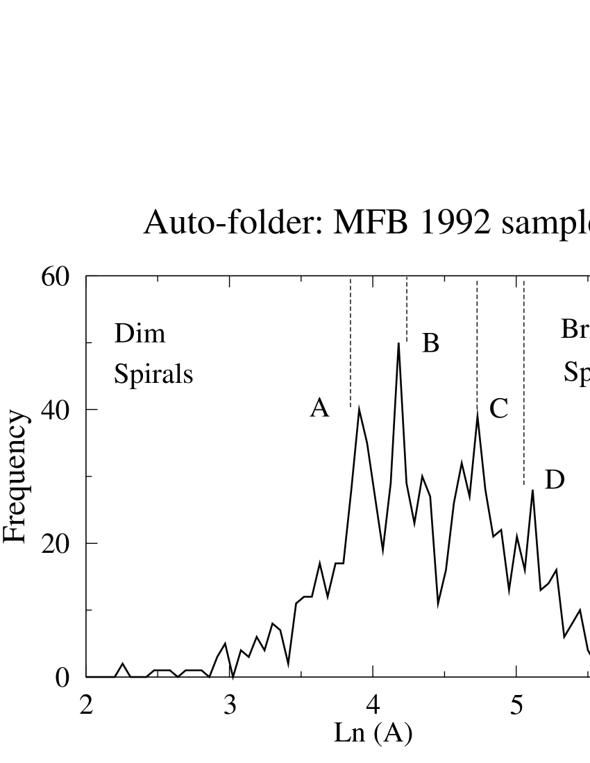
Figure 2: $\ln A$ distribution for the Mathewson et al Mathewson1992 (1992) sample with auto-folding and original Mathewson et al TF scaling; Vertical dotted lines indicate peak centres of Persic & Salucci solution. Bin width = 0.055

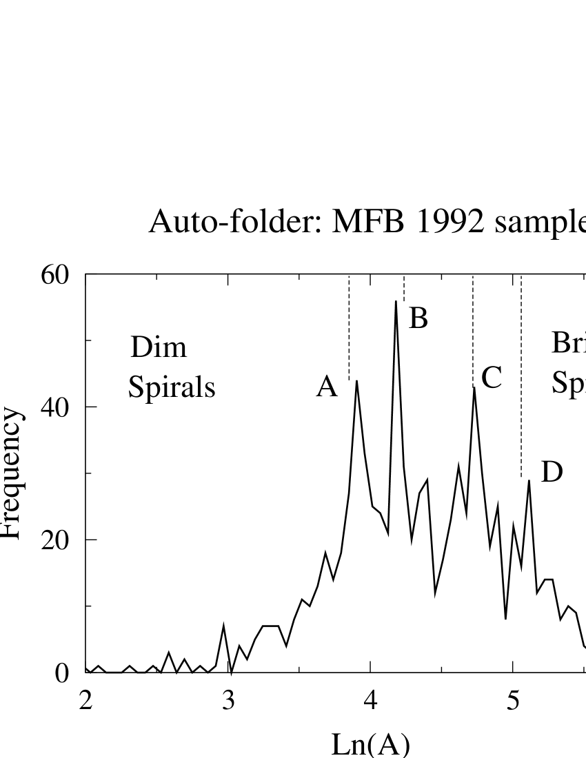
Figure 3: $\ln A$ distribution for the Mathewson et al Mathewson1992 (1992) sample with auto-folding and rescaled TF; Vertical dotted lines indicate peak centres of Persic & Salucci solution. Bin width = 0.055

The vertical dotted lines in this latter figure mark the positions of the peaks $A,\,B,\,C,\,D$ of the Persic & Salucci Persic1995 (1995) solution, in figure 1. It can therefore be seen that the peak structure revealed by the Persic & Salucci Persic1995 (1995) folding method is not an artifact of their method, but is an objective feature on the Mathewson et al Mathewson1992 (1992) sample.

4.2 The effect of rescaling the TF relation within the error bars

According to the diagnostic magnitude mapping, (2), the reference range of TF magnitudes generated by the scaling (1) is compressed and shifted to the dim end relative to the Hubble magnitudes. This suggests that a possible rescaling designed to expand the reference range of TF magnitudes could be considered. Such an expansion, consistent with Mathewson et al’s original calibration, is obtained by steepening the TF gradient within the quoted error bars. We find that, if the peak structure is to be optimized, then a steepening of the gradient (in the negative sense) must be accompanied by a reduction in the zero point. The overall process is completed by an ‘eye-ball’ iteration which can be described as follows:

1. Guess a new gradient value within the quoted error bar;

2. Adjust the zero point to maximise the peak structure for this gradient;

3. Perform the diagnostic magnitude mapping, adjusting $H$ as necessary to get the best match at any given iteration;

4. Repeat until a satisfactory magnitude mapping is obtained.

We find

$$M=-8.30\,\log V_{rot}-2.56,$$ (3)

gives the magnitude mapping

$$(-23.3,-18.2)_{H95}\leavevmode\nobreak\ \rightarrow\leavevmode\nobreak\ (-23.2,-18.2)_{TF}\,$$ (4)

computed with $H=95\,$km/sec/Mpc. There is now no significant magnitude bias or shifting. The corresponding $\ln A$ frequency map is given in figure 3, and we see a small increase in signal strength on all four peaks. In summary, the combined effects of the improved magnitude mapping, together with the increase in the strength of the $\ln A$ peak structure suggest that the recalibration (3) is justified.

4.3 The effect of excluding the edge-on galaxies

In practice, we find that excluding the edge-on galaxies, which are about 17% of the sample, has the effect of producing only a pro-rata reduction in the heights of the peaks in figure 2. In other words, the inclusion of the edge-on galaxies in the present analysis has a neutral effect upon it. The reason for this result is almost certainly that the effects of internal absorption are considerably greater on the interior parts of ORCs than they are on the exterior parts, and it is precisely these parts which are discarded in the data reduction process described in §3 for the computation of $(\alpha,\,\ln A)$.

5 The analysis of the Dale, Giovanelli, Haynes & Uson sample

From our point of view, the value of the work of Dale et al Dale1997 (1997) et seq lies in its provision of a rotation curve sample which is completely independent in all of its aspects of the Mathewson et al samples.

As a general comment, it is to be noted that part of the explicit general programme of Giovanelli, Haynes et al has been to develop a highly accurate Tully-Fisher $I$-band ‘template’ relation for the purpose of establishing a cluster inertial frame out to $z\approx 0.06$. Thus, Giovanelli et al Giovanelli (1997) are able to quote the very tight error bars of $\pm 0.02$ for their TF gradient determinations. To ensure such accuracy, much effort has been put into establishing a reliable linewidth estimation technique. This technique, which is described by Dale et al Dale1998 (1998), is an algorithmic approach based on the estimate $V_{90\%}-V_{10\%}$ first introduced by Dressler & Faber Dressler (1990). However, it should be noted that this definition is most reliable when ORCs extend out to at least $R_{83}$, the optical radius as defined by Persic & Salucci Persic1995 (1995). The reason is that, as Dale et al Dale1998 (1998) point out, the definition then recovers $V_{opt}$ in a reliable way and, as Persic & Salucci Persic1991 (1991, 1995) have shown, $V_{opt}$ provides a reasonable basis for linewidth definitions. To deal with those ORCs which were insufficiently extensive, Dale et al Dale1998 (1998) introduced an elaborate procedure which involved the use of $N_{II}$ measurements to calculate a parameter, called a ‘shape factor’, for each ORC. This shape factor was subsequently used to extrapolate ORCs out to $R_{83}$ and to correct raw $V_{90\%}-V_{10\%}$ linewidths as necessary.

5.1 The Dale et al calibration of Tully-Fisher

The Dale et al Dale1998 (1998) calibration of the Tully-Fisher relation is given by

$$M_{TF}=-7.68\,(\pm 0.02)\,\log V_{rot}-4.12+5\,\log h$$ (5)

where $H=100h\,$km/sec/Mpc is undetermined. The error bars on the gradient are so tight that, effectively, there is no freedom to vary the estimated TF gradient. However, the analysis of the Mathewson et al sample in §4 strongly suggest a value $H=95\,$km/sec/Mpc so that $h=0.95$ in (5). Thus the suggested calibration is given by

$$M_{TF}=-7.68\log V_{rot}-4.23,$$ (6)

and the corresponding $\ln A$ frequency diagram is given in figure 4. We see that the predicted peak structure is strongly reproduced. Similarly, the diagnostic magnitude mapping is given by

$$(-23.3,-18.2)_{H95}\rightarrow(-23.2,-18.1)_{TF}$$

which, apart from a very slight uniform shift to the dim, indicates the complete absence of any systematic magnitude bias.

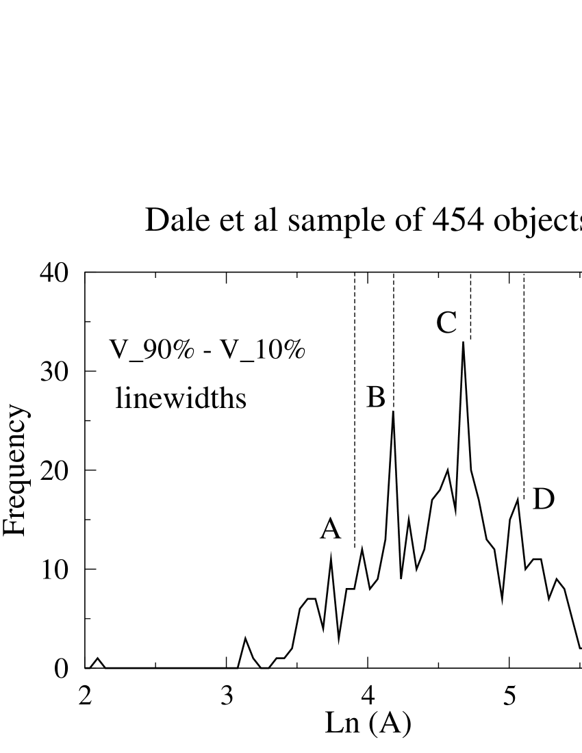
Figure 4: The $\ln A$ distributions for the Dale et al sample, with auto-folder and using the Dale et al TF calibration for $H=95\,km/sec/Mpc$. Vertical dotted lines indicate peak centres of figure 2. Bin width = 0.055

5.2 The effect of excluding the edge-on galaxies

About 11% of the Dale et al sample consists of edge-on galaxies, and the effect of excluding these galaxies is the same as for the previous two samples - that is, there is merely a pro-rata reduction in the peak heights.

6 The Analysis of the Mathewson & Ford Mathewson1996 (1996) sample

The Mathewson & Ford Mathewson1996 (1996) sample, like the Mathewson et al Mathewson1992 (1992) sample, is also drawn from an area of the sky which contains the, so-called, GA and approximately one half of the Mathewson & Ford Mathewson1996 (1996) sample lies within the GA region, $260^{o}<l<360^{o},-40^{o}<b<45^{o}$ but, as reference to table 3 shows, is an average of 70% more distant than the Mathewson et al Mathewson1992 (1992) sample and is therefore considerably less bright.

6.1 The Mathewson et al calibration for MF data

A direct application of the Mathewson et al Mathewson1992 (1992) TF calibration, given at (1), to the Mathewson & Ford Mathewson1996 (1996) sample gives the $\ln A$ frequency diagram of figure 5.

Figure 5: The $\ln A$ distributions for the Mathewson & Ford Mathewson1996 (1996) sample with auto-folding using Mathewson linewidth estimates and original TF calibration. Vertical dotted lines indicate peak centres of figure 2. Bin width = 0.055

This figure shows that, whilst the $B$, $C$ and $D$ peaks are reproduced, the distribution is extremely noisy and must be considered poor. Given the quality of the results obtained from the Mathewson et al Mathewson1992 (1992) sample, and shown in figures 2 and 3, we can suppose that some kind of problem exists.

As a possible means of understanding what the problem might be, we consider the subsample of Mathewson & Ford Mathewson1996 (1996) data which is exterior to the GA region (discussed in §4) and calculate how the reference range of Hubble magnitudes maps into Tully-Fisher magnitudes for this data. Using the original Mathewson TF calibration (for which $H=85\,$km/sec/Mpc), we find the diagnostic magnitude mapping for non-GA objects

$$(-23.3,-18.2)_{H85}\leavevmode\nobreak\ \rightarrow\leavevmode\nobreak\ (-23.0,-17.4)_{TF}$$ (7)

which implies the existence of a very strong systematic bias which shifts the whole Mathewson & Ford Mathewson1996 (1996) sample to lower luminosities. This is improved at the bright end when our modified Mathewson TF calibration (3) is used, but the dim-end bias remains essentially unchanged.. Given that the non-GA objects are not believed to be participating in any large-scale flow, there are two basic possibilities for explaining the mapping (7) which can be listed as

• The MF Hubble luminosities are very much overestimated at the dim end;

• The MF Tully-Fisher luminosities are very much underestimated at the dim end.

The first possibility seems unlikely since Mathewson & Ford Mathewson1996 (1996) photometry is in the $I$ band for which the internal and external extinction mechanisms are well understood, and for which well-tested correction techniques exist and have been applied by Mathewson & Ford Mathewson1996 (1996). The second possibility would necessarily have its source in the systematic underestimation of dim-end optical linewidths for this relatively distant sample. Since Mathewson & Ford Mathewson1996 (1996) (and Mathewson et al Mathewson1992 (1992)) used an intuitive ‘eyeball’ technique for linewidth estimation, this latter possibility seems the most likely explanation. On the basis of the working hypothesis that Mathewson & Ford’s linewdith estimates are subject to a systematic bias relative to the Mathewson et al Mathewson1992 (1992) linewidths, there are now two possible ways to proceed:

1. We can either derive our own linewidth estimates directly from the sample using some algorithmic technique;

2. Or we can take advantage of the idea that, where systematic linewidth bias exists, it can accounted for by a compensating recalibration of the Tully-Fisher relation.

We consider both of these approaches in the following sections.

6.2 TF based on $V_{opt}$ linewidths

The first approach is based on the idea of generating our own linewidth estimates. The most simple algorithmic technique for linewidth estimation is that based on $V_{90\%}-V_{10\%}$. However, as discussed in §5, linewidths based on this definition can only reliably be used when ORCs extend out to at least to the optical radius, and Dale et al used an elaborate procedure to negotiate this problem for those ORCs which did not. This approach is not possible in the present case because the required $N_{II}$ measurements are not available for Mathewson data. But Dale et al Dale1998 (1998) also report that their definition of linewidth recovers Persic & Salucci’s $V_{opt}$ whenever ORCs are sufficiently extensive. This implies that using $V_{opt}$ as a tentative linewidth definition for Mathewson & Ford data should allow a TF calibration very similar to that of Dale et al’s given at (6).

However, although $R_{83}$ (angular measure) estimates are provided with the Mathewson & Ford Mathewson1996 (1996) sample, the corresponding $V_{opt}$ are not. We circumvent this problem by using the power-law $V=A\,R^{\alpha}$ fitted to the folded, but as yet unscaled, ORC to estimate $V_{opt}$ at $R_{83}$ (angular measure). This process is possible prior to scaling simply because $\alpha$ values are independent of scaling. With these linewidths, we find that the exact Dale et al calibration (5) with a zero point of $-4.08$,

$$M=-7.68\log V_{rot}-4.08,$$

gives the $\ln A$ frequency diagram of figure 6. By contrast with figure 5, we see that the whole $A,B,C,D$ peak structure is now very well reproduced. Interestingly, and as judged by the absence of any bias in magnitude mapping

$$(-23.3,-18.2)_{H85}\leavevmode\nobreak\ \rightarrow\leavevmode\nobreak\ (-23.2,-18.3)_{TF},$$

this latter TF calibration corresponds more closely to $H=85\,$km/sec/Mpc for the non-GA Mathewson & Ford Mathewson1996 (1996) subsample than the higher value of $H=95\,$km/sec/Mpc.

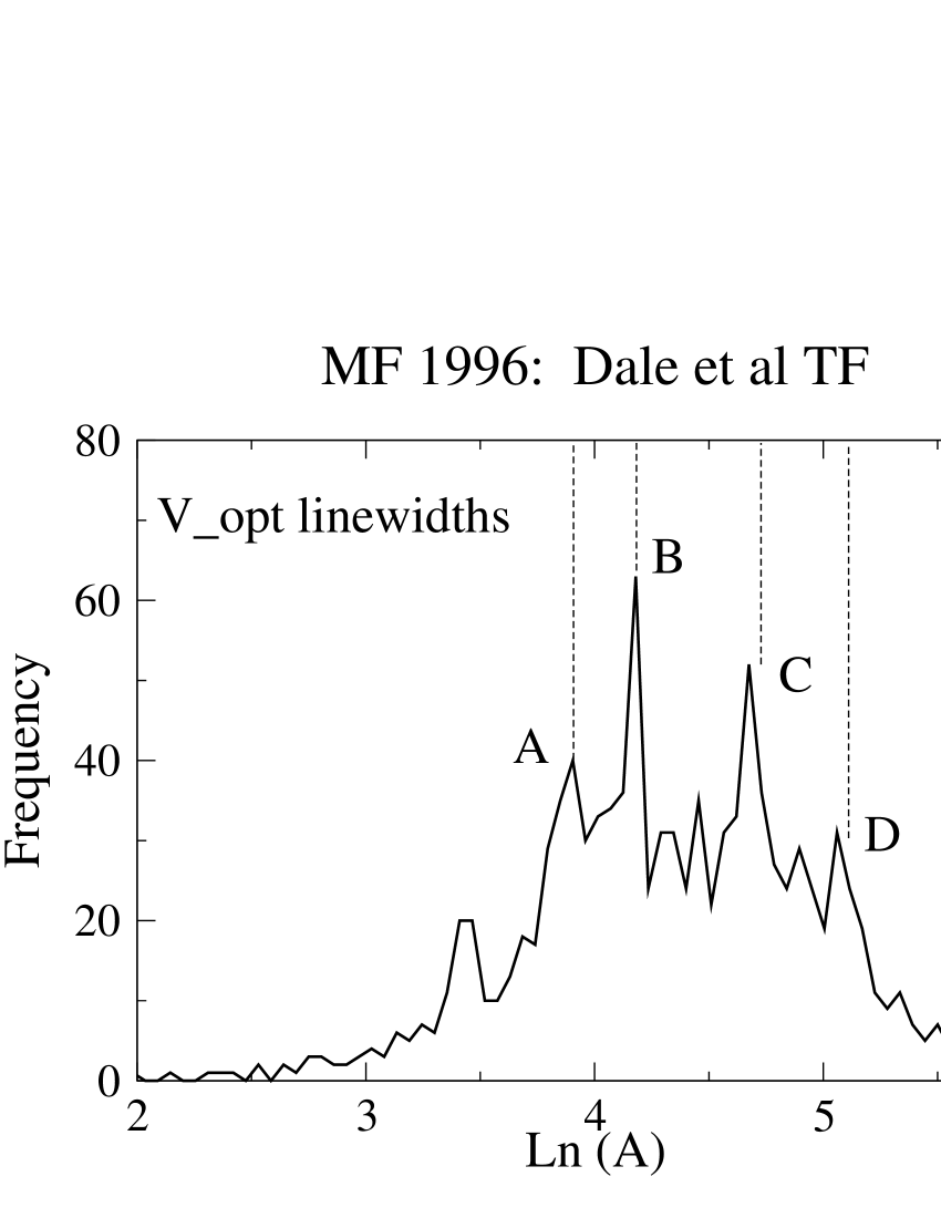
Figure 6: The $\ln A$ distributions for the Mathewson & Ford Mathewson1996 (1996) sample with auto-folding using $V_{opt}$ linewidths and Dale et al TF calibration with shifted zero point. Vertical dotted lines indicate peak centres of figure 2. Bin width = 0.055

6.3 Linear rescaling of TF for linewidth bias-correction

The relative success of the $V_{opt}$ linewidth estimate provides further circumstantial evidence for the working hypothesis that the Mathewson & Ford linewidths are, in fact, systematically biased. We make the simplest possible assumption that such a bias can be accounted for by a linear recalibration of the TF relation designed to ensure that the diagnostic magnitude mapping is bias-free. We find that the rescaled TF relation

$$M_{TF}=-7.46\log V_{rot}-4.85,$$ (8)

gives the $H=88\,$km/sec/Mpc diagnostic magnitude mapping

$$(-23.3,-18.2)_{H88}\leavevmode\nobreak\ \rightarrow\leavevmode\nobreak\ (-23.3,-18.2)_{TF},$$ (9)

for non-GA ORCs, which is perfect. Corresponding to this improvement, we find that the recalibration (8) gives the $\ln A$ frequency diagram of figure 7 which is likewise a considerable qualitative improvement over figure 5. In particular, the $A$ and $B$ peaks are now perfectly and strongly reproduced, whilst the $C$ peak is clearly present, but noisy. The $D$ peak is virtually non-existent.

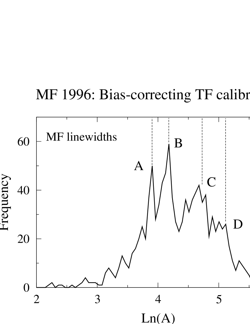
Figure 7: The $\ln A$ distributions for the Mathewson & Ford Mathewson1996 (1996) sample with auto-folding using the TF recalibration with linear rescaling. Vertical dotted lines indicate peak centres of figure 2. Bin width = 0.055

6.4 The effect of excluding the edge-on galaxies

Only about 6% of the Mathewson & Ford (1995) sample consists of edge-on galaxies, and the effect of excluding these galaxies is the same as for the Mathewson et al Mathewson1992 (1992) sample - that is, there is merely a pro-rata reduction in the peak heights.

7 The analysis of the Courteau Courteau (1997) sample

As with the Dale et al sample, the value of the Courteau sample lies in its complete independence in all of its aspects of the Mathewson et al samples.

The Courteau Courteau (1997) analysis was primarily designed to address the problem of linewidth definitions, with a view to obtaining a standardized objectively defined algorithmic definition. Courteau considered several possibilities for linewidth definitions, and we present results using his $V_{max}$ and $V_{2.2}$ definitions (his estimated ‘worst’ and ‘best’ respectively). Because his explicit concern was to make a comparative investigation of several linewidth estimation techniques, less effort was expended in establishing particularly accurate TF calibrations for each of the linewidth estimates considered. For example, unlike Mathewson et at Mathewson1992 (1992) or Dale et al Dale1998 (1998), Courteau did not calibrate his Tully-Fisher relations on specially chosen low-redshift dispersion clusters, but on his whole sample, which has a redshift dispersion in excess of $10000\,$km/sec. It follows that his calibrations are not likely to be as accurate as those of Mathewson et al Mathewson1992 (1992) and Giovanelli et al Giovanelli (1997). Thus, Courteau’s quoted error bars on gradient determinations for each of the linewidth estimators considered are, typically, $\pm 0.2$, which is to be compared with Giovanelli et al’s Giovanelli (1997) quoted error bar of $\pm 0.02$.

7.1 The Courteau calibrations of Tully-Fisher for two linewidths

7.1.1 The $V_{max}$ linewidth TF calibration

The Courteau Courteau (1997) calibration of the Tully-Fisher relation for his $V_{max}$ linewidths, using his $H=70\,$km/sec/Mpc, is given by

$$M_{TF}=-6.09\,(\pm 0.26)\,\log V_{max}-7.22$$

where the gradient error bar is as given by Courteau. We subsequently find that the recalibration

$$M_{TF}=-6.19\log V_{max}-7.50$$

gives the $\ln A$ frequency diagram of figure 8. Except for the $A$ peak which is non-existent because of lack of data at the dim end of the Courteau sample, we see that the peak structure of the hypothesis is very well reproduced - although it is much noisier than the peak structures of Mathewson et al and Dale et al shown in figures 3 and 4 respectively. Note that the recalibrated gradient is comfortably within Courteau’s quoted error bar.

It is also of interest to note that the net effect of the recalibration is to increase the luminosity of the average galaxy by about $0.48$ magnitudes. This is well within Courteau’s quoted error bar for $V_{max}$ calibrations of $0.55$ magnitudes and so there is no evidence to suggest that the recalibration is significantly different from Courteau’s original $V_{max}$ calibration which assumed $H=70\,$km/sec/Mpc.

7.1.2 The $V_{2.2}$ linewidth TF calibration

The Courteau Courteau (1997) calibration of the Tully-Fisher relation for his $V_{2.2}$ linewidths, using his $H=70\,$km/sec/Mpc, is given by

$$M_{TF}=-6.36\,(\pm 0.22)\,\log V_{2.2}-6.78\,.$$

We find that the recalibration

$$M_{TF}=-6.55\log V_{2.2}-7.15$$

gives the $\ln A$ frequency diagram of figure 9. Except for the $A$ peak which is non-existent because of lack of data at the dim end of the Coruteau sample, we see that the peak structure of the hypothesis is, again, reasonably well reproduced. Note that the recalibrated gradient is within Courteau’s quoted error bar.

This time, the net effect of the recalibration is to increase the luminosity of the average galaxy by about $0.77$ magnitudes. This is well outside Courteau’s quoted error bar for $V_{2.2}$ calibrations of $0.46$ magnitudes. Since the recalibrated gradient has not changed significantly, this result is consistent with the idea that the recalibrated zero point is significantly different from Courteau’s original value for the $V_{2.2}$ calibration.

7.2 An oddness in the Courteau sample

As a consistency check on the $V_{max}$ calibration, we note that the application of this calibration to the Courteau sample with $H=70\,$km/sec/Mpc gives the magnitude mapping

$$(-23.3,-18.2)_{H70}\rightarrow(-23.0,-19.7)_{TF}.$$

Thus, we see that Courteau’s $V_{max}$ calibration compresses the magnitude range by about 35%, with the dim end being too luminous by $1.5$ whole magnitudes. It is easy to see that varying the Tully-Fisher zero point will simply have the effect of shifting the given TF range $(-23.0,-19.7)_{TF}$ either up or down - but it cannot expand the range to match the Hubble range.

Similarly, a consistency check on the $V_{2.2}$ calibration, with $H=70\,$km/sec/Mpc gives the magnitude mapping

$$(-23.3,-18.2)_{Hubble}\rightarrow(-23.6,-19.6)_{TF}.$$

The only way to get a match in either case is to vary both the gradient and the zero point in the Tully-Fisher relation. We find that a good mapping can only be had with TF calibrations similar to

$$M=-9\log_{10}V_{rot}-1.$$

But the gradient here, $-9$, is well outside of the envelope of typical $R$-band TF gradients and can only be considered as extreme. Given that Courteau’s Courteau (1997) study was primarily designed to investigate algorithmic definitions of linewidths, and that he judged his $V_{2.2}$ linewidths to be on a par with $H_{I}$ linewidths, it would seem that the only likely explanation for the problem lies in the possibility that the sample of chosen galaxies is not quiet in the Hubble sense.

7.3 The effect of excluding the edge-on galaxies

Less that 1% of the Courteau sample consists of edge-on galaxies, and so there is no discernible effect arising from their exclusion.

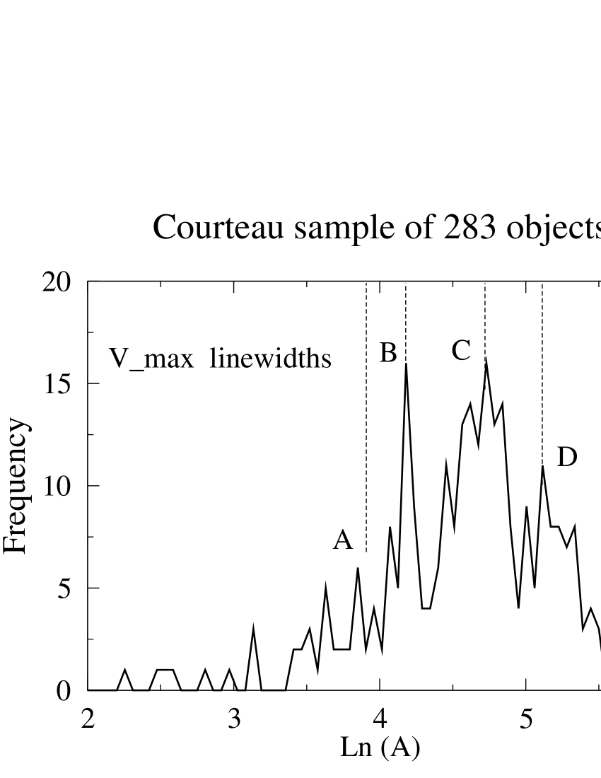
Figure 8: The $\ln A$ distributions for the Courteau Courteau (1997) sample using his $V_{max}$ linewidth definition and $H=70\,$km/sec/Mpc. Vertical dotted lines indicate peak centres of figure 2. Bin width = 0.055

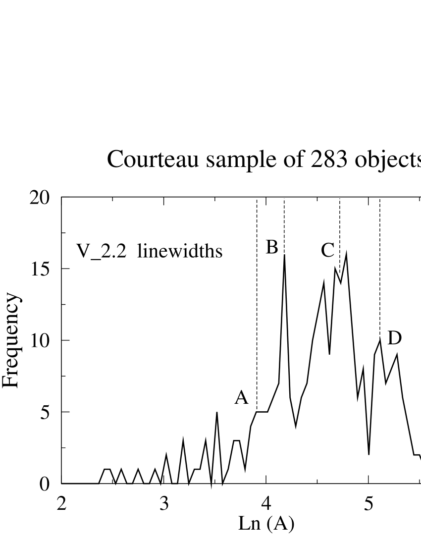
Figure 9: The $\ln A$ distributions for the Courteau Courteau (1997) sample using his $V_{2.2}$ linewidth definition and $H=70\,$km/sec/Mpc. Vertical dotted lines indicate peak centres of figure 2. Bin width = 0.055

8 The statistical significance of the various analyses

We begin with a broad overview of the various analyses: the results of the foregoing analyses, already encapsulated in figures 2, 3, 7, 4, 9 and 8, are collected together for convenient comparison in table 4. The refined specific hypothesis to be defined and tested states, briefly, that strong peaks in $\ln A$ frequency diagrams of rotation curve data processed in the way described, should occur coincidently with the peaks $A,\,B,\,C$ and $D$ in figure 2, which has been derived from our autofolder analysis of Mathewson et al (1992) data. The exact bin-centre positions in which these latter peaks lie are given in the first row of table 4, whilst remaining five rows give the peak centres for the remaining figures. The table makes it clear that the peak positions are essentially identical across the four samples. In the following, we provide a standardized quantitative estimate of the statistical significance of these results.

Table 4: Comparison of peak positions in $\ln A$ frequency diagrams for MFB, MF, DGHU & SC data

Sample	A	B	C	D
MFB	3.91	4.18	4.73	5.12
${\rm MF}_{Vopt}$	3.91	4.18	4.68	$5.06$
${\rm MF}_{Vorig}$	3.91	4.18	4.68	$-$
DGHU	$-$	4.18	4.68	5.06
${\rm SC}_{Vmax}$	$-$	4.18	4.73	5.12
${\rm SC}_{V2.2}$	$-$	4.18	$4.73^{*}$	$5.12$
$\leavevmode\nobreak\ {}^{*}$ indicates average over three points
$-$ indicates no significant peak

8.1 A standardized methodology

We noted, in §1, that an extremely conservative upper-bound estimate of the probability of the peaks in figure 1 occurring by chance alone, given the prior hypothesis raised on the Rubin et al Rubin (1980) data, was given in Roscoe 1999a to be less than $10^{-7}$. However, this estimate was derived using a crude ad-hoc methodology, and applied specifically to the Persic & Salucci folding solution of the Mathewson et al (1992) data. For the purpose of enabling statistical comparison across our whole analysis, we introduce a standardized methodology - which is already partly implemented - and apply it where possible to each sample. Specifically:

• require that all samples to be tested are processed (folding etc), as far as is possible, in an identical fashion;

• define the null hypothesis that all samples are drawn from the same background distribution, and that this latter distribution is smooth - that is, has no peak structure;

• set up the specific hypothesis to be tested, and test it via a Monte-Carlo simulation which randomly selects a very large number of samples from the hypothetical smooth distribution.

The first of these points is, of course, already implemented. For the second point, experimentation shows that the final outcomes are insensitive to any reasonable choice of ‘smooth distribution’ for the null hypothesis; we define it as the cubic spline envelope of the figure 2 distribution shown in figure 10. For the third point, the Mathewson et al Mathewson1992 (1992) sample must be tested against the original hypothesis raised on our analysis of the Rubin et al Rubin (1980) sample, whilst our additional samples will be tested against a refined hypothesis raised on the analysis of the Mathewson et al Mathewson1992 (1992) sample.

8.2 Significance of the Mathewson et al Mathewson1992 (1992) results: Figure 2

In essence, we shall revise the original crude ad-hoc estimates of the significance of the peaks arising from the Persic & Salucci folding of Mathewson et al Mathewson1992 (1992) data, shown in figure 1, given the original hypothesis raised on the Rubin et al Rubin (1980) data described in §1. Briefly, this original hypothesis stated that, using Rubin scaling, then $\ln A$ would lie within $\pm 0.15$ of integer or half-integer values - specifically, the values 3.5, 4.0, 4.5 and 5.0. The transformation of these Rubin-scaled intervals to the scaling used by Mathewson et al Mathewson1992 (1992) is given in table 5.

Figure 10: Hypothetical smooth $\ln A$ distribution, defined as a cubic spline envelope of actual MFB 1992 distribution. Bin width = 0.055

Table 5: $\ln A$ interval transformation

Interval with	Interval with	Associated
RFT scale	MFB scale	peak
$(\,3.35,\,3.65\,)$	$(\,3.69,\,3.93\,)$	$A$
$(\,3.85,\,4.15\,)$	$(\,4.10,\,4.34\,)$	$B$
$(\,4.35,\,4.65\,)$	$(\,4.51,\,4.75\,)$	$C$
$(\,4.85,\,5.15\,)$	$(\,4.92,\,5.16\,)$	$D$

Table 6: Test of peak-structure in figure 2

Peak frequencies in $10^{6}$ trials
Interval with	Frequency at	Peak
MFB scale	required	label
	strength
$(\,3.69,\,3.93\,)$	$3513$	$A$
$(\,4.10,\,4.34\,)$	$758$	$B$
$(\,4.51,\,4.75\,)$	$18881$	$C$
$(\,4.92,\,5.16\,)$	$66303$	$D$
Probability of four sufficiently strong peaks
appearing in the same trial $\approx\,3\times 10^{-9}$

The required probability estimate for the peaks of figure 2 was obtained by generating $10^{6}$ randomly selected samples of 866 measurements each (the number of auto-foldable ORCs in the Mathewson et al Mathewson1992 (1992) sample) from the hypothetical smooth distribution of figure 10, and counting how many times peaks of the observed (or greater) sizes actually occur in the intervals specified in table 5. The frequency at which peaks of the required size actually appeared is given in table 6. On no occasion did more than two peaks at the required strengths appear in the same trial; however, assuming independent probabilities, the observed frequencies allow us to estimate that the probability of four peaks of the required strengths appearing simultaneously to be estimated at $3\times 10^{-9}$.

8.3 A refined hypothesis for the new samples

The considerations of §8.2 allow us to refine the hypothesis tested there (which arose from a consideration of just 12 Rubin et al Rubin (1980) objects) as follows: The distribution of $\ln A$, computed for folded ORCs according to the prescription of §3, will show significant peak structure with peaks centred on the $\ln A$ values $(3.91,4.18,4.73,5.12)$, where 90% confidence limits on the positions of these peaks, calculated in detail in Appendix D, are given approximately by $(3.87,3.98)$, $(4.15,4.21)$, $(4.70,4.76)$ and $(5.09,5.14)$ respectively.

Table 7: Test of peak-structure probabilities using the refined hypothesis of §8.3

	Peaks at observed strength in $10^{6}$ simulations				Single trial
	A	B	C	D	probability
Fig4 (Dale)	$-$	11797	3	23010	$8\times 10^{-10}$
Fig6 (MF $V_{opt}$)	28106	131	1204	70559	$3\times 10^{-10}$
Fig7 (MF $V_{orig}$)	192	1024	93262	$-$	$2\times 10^{-8}$
Fig8 (SC $V_{max}$)	$-$	44889	8098	34653	$1\times 10^{-5}$
Fig9 (SC $V_{2.2}$)	$-$	44918	17452	71252	$6\times 10^{-5}$
$-$ indicates non-existent peak.

8.4 The significance of the Dale et al results: Figure 4

The error bars given by Giovanelli et al Giovanelli (1997) for their TF gradient estimate were so tight ($\pm 0.02$) that, effectively, there was no freedom to vary this parameter. Similarly, the $H=95\,$km/sec/Mpc value used to fix the TF zero point arose directly from optimizing the results of the Mathewson et al Mathewson1992 (1992) analysis given in §4. Effectively, therefore, the $\ln A$ frequency diagram of figure 4 arose from a single trial and, accordingly, the associated probabilities can be calculated directly from the figure on the basis of the modified hypothesis of §8.3.

The procedure is as before, except that each randomly selected sample now contains 454 measurements each - which is the number of auto-foldable ORCs in the Dale et al sample - and the results are shown in table 7. Assuming independent probabilities, the observed frequencies allow us to estimate that the probability of the three peaks listed appearing simultaneously at the observed magnitudes in figure 4 to be estimated at $8\times 10^{-10}$. However, it is obvious from table 7 that most of the power in this latter result arises from the extreme naure of peak $C$. But, even if the number of peak $C$ occurrences equalled the number of peak $D$ occurrences, the single-trial probablility for this case would still be insignificant at $6\times 10^{-6}$.

8.5 The significance of Mathewson & Ford Mathewson1996 (1996) results: Figure 6

We now calculate the significance of the peak structure arising from our analysis of Mathewson & Ford Mathewson1996 (1996) data - exhibited in figure 6 for the $V_{opt}$ linewidth results - given the modified hypothesis of §8.3. The procedure is as before, except that each randomly selected sample now contains 1085 measurements each - which is the number of auto-foldable ORCs in the Mathewson & Ford Mathewson1996 (1996) sample - and the results are shown in table 7.

Assuming independent probabilities, the observed frequencies allow us to estimate that the single-trial probability of four peaks of the required strengths appearing simultaneously to be estimated at $3\times 10^{-10}$. However, in this particular case:

• We allowed ourselves the freedom to use an alternative linewidth estimation method when the original linewidths of Mathewson & Ford Mathewson1996 (1996), which gave rise to figure 5, were inferred to be problematical;

• Whilst, for the alternative method we used the Giovanelli et al gradient value for the TF calibration, we allowed ourselves the freedom to search for a new zero point. Discounting the fact that we were guided by the magnitude mapping technique, it is a fair assessment to say that, typically, the search for a suitable zero point required about five further independent trials.

To make a round figure, suppose then that the figure 6 results required ten independent trials to obtain. On this basis, we can use the single-trial probability and binomial statistics to estimate the required probability at $3\times 10^{-9}$.

8.6 The significance of the Courteau results: Figures 9

The estimation of the probabilities attached to the Courteau results is a little more involved than the other two case. Briefly, we argue as follows:

• We chose at the outset to consider only the $V_{max}$ and $V_{2.2}$ Courteau linewidth estimates. So there are two degrees of freedom arising here;

• For each of the linewidth estimates, the error bars quoted by Courteau for the gradients are approximately $\pm 0.2$. Given that we allow ourselves the freedom to vary the gradient within the quoted error bars, this amounts to about three independent trials to optimize the gradient value per linewidth estimate;

• Finally, we allowed ourselves the freedom to determine the zero points for each of the TF calibrations. Typically, each zero point determination required five trials for a given gradient determination.

So, for each linewidth estimate, we can reasonably say that fifteen independent trials were required to determine the optimal TF calibration - making thirty independent trials in all. Given the single-trial probability of $1\times 10^{-5}$ from table 7 for the $V_{max}$ linewidth analysis, we can use binomial statistics to estimate the overall probability of obtaining the figure 8 results by chance alone at about $3\times 10^{-4}$.

8.7 Summary of statistics

A hypothesis was raised on the basis of a simple analysis of 12 Rubin et al Rubin (1980) galaxies; this hypothesis was tested against the results obtained from a sample of 866 Mathewson et al Mathewson1992 (1992) ORCs and it was confirmed with a probability of $\approx 3\times 10^{-9}$ against the obtained results arising purely by chance.

The analysis of this larger sample of 866 ORCs allowed a refinement of the hypothesis, which was subsequently tested against the results obtained from three new independent samples of 454 ORCs with $I$-band photometry from Dale et al Dale1997 (1997) et seq, 1085 ORCs with $I$-band photometry from Mathewson & Ford Mathewson1996 (1996) and 283 ORCs with $R$-band photometry from Courteau Courteau (1997). The probabilities of the results obtained from each of these samples arising by chance alone were estimated at $8\times 10^{-10}$, $3\times 10^{-9}$ and $3\times 10^{-4}$ respectively. On the basis of these results, it is reasonable to say that the ‘discrete dynamical classes’ hypothesis for spiral discs has been verified at the level of virtual certainty.

9 A second generation of Tully-Fisher methods.

At a practical level, the foregoing analysis has implications concerning the general nature of Tully-Fisher methods which we shall expand upon in this section. These can be summarized as:

1. The discrete dynamical states phenomonology provides an absolute standard whereby Tully-Fisher methods can be absolutely calibrated on a large enough sample;

2. The Tully-Fisher method is shown to have two equivalent formulations, one of which is the familar one;

3. The Tully-Fisher relation is shown to be augmented by a corresponding relation which defines where on an ORC a linewidth should be measured. Thus, a means is provided whereby Tully-Fisher calibrations and linewidth determinations can, in principle, be algorithmically, absolutely and simultaneously determined from any given large sample of ORCs;

4. The concept of ‘linewidth’ is shown to be not absolute - that is, linewidth can be defined with virtually unlimited freedom. But, once defined, the form of the corresponding Tully-Fisher calibration becomes fixed.

9.1 The essential background

The consequences listed above rest upon the assumption that the power-law analysis can be shown to provide a high-quality resolution of ORC data in that part of the disc where the discrete dynamical classes phenomonology manifests itself. To demonstrate this, the first thing of significance to be considered is the $(\alpha,\,\ln A)$ plot, given in figure 11 for the combined Mathewson et al Mathewson1992 (1992), Mathewson & Ford Mathewson1996 (1996), Dale et al Dale1997 (1997) et seq samples of 2405 objects having $I$-band photometry and reliably foldable ORCs.

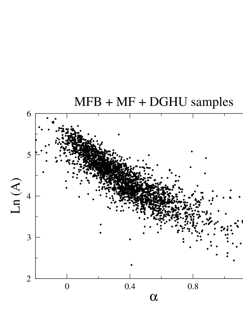
Figure 11: Plot of $(\ln A,\,\alpha)$ for 2405 galaxies

Table 8: $\ln A$ model

Variable	Coeff	t ratio
${\rm const}$	$-1.596$	$-11$
$M$	$-.316$	$-46$
$S$	$-0.0002$	$-2$
$\alpha$	7.614	28
$\alpha\,M$	0.474	34
$\alpha\,S$	0.0050	18
N=1951; $R^{2}=92\%$

We now make a detailed analysis of the 1951 $(\alpha,\,\ln A)$ points in figure 11 which are associated with the specific subset of the Mathewson et al 1992 + Mathewson & Ford 1995 ORCs. In the context of the model

$${V\over V_{0}}=\left({R\over R_{0}}\right)^{\alpha}\leavevmode\nobreak\ \leavevmode\nobreak\ \longrightarrow\leavevmode\nobreak\ \leavevmode\nobreak\ A={V_{0}\over R_{0}^{\,\alpha}}\,,$$ (10)

we find

$$\ln A = \ln\,V_{0}-\alpha\,\ln\,R_{0}$$ (11)

$$= -1.596-0.316\,M+7.614\,\alpha+0.474\,\alpha\,M$$

$$+0.0050\,\alpha\,S$$

for the two $I$-band Mathewson samples. Here $M$ is absolute magnitude, and $S$ is surface brightness defined as average solar luminosities per square parsec for the whole area inside the optical radius, $R_{83}$, as defined by, for example, Persic & Salucci Persic1995 (1995). This particular model was obtained by using the original Mathewson linewidths for the Mathewson et al Mathewson1992 (1992) sample, and the $V_{opt}$ linewidths for the Mathewson & Ford Mathewson1996 (1996) sample, and by rejecting all $3\,\sigma$ outliers (about 4% of the total), and it accounts for about 92% of the variation in figure 11. The detailed statistics are given in table 8 and it is clear that, except for surface brightness, $S$, all of the chosen predictors have an extremely powerful effect in the model.

9.2 Extraction of models for $\ln R_{0}$ and $\ln V_{0}$

Introducing the ‘discrete dynamical states’ phenomonology into the discussion, we now note that the model can be decomposed into separate expressions for $(\ln R_{0},\ln V_{0})$ according to

$$\ln A_{i} = \ln V_{0}-\alpha\,\ln R_{0},\leavevmode\nobreak\ \leavevmode\nobreak\ i=1,2,3,4$$

$$\ln V_{0} = -1.596-0.316\,M+\Gamma$$ (12)

$$\ln R_{0} = -7.614\,-0.474\,M-0.0050\,S+{\Gamma\over\alpha}$$

where $\ln A_{i}\,=\,3.91,\,4.18,\,4.73,\,5.12$ and denotes the positions of the $A,B,C,D$ peaks, and $\Gamma$ is an arbitrary function (or parameter) arising from the decomposition of $\ln A_{i}$. It is easily verified that (10) is invariant with respect to an arbitrary choice of this $\Gamma$.

An effective visual verification of the fit of model (12) is obtained by noting that if we use the definitions of (12) in the dimensionless form of (10), and then regress $\ln(V/V_{0})$ on $\ln(R/R_{0})$, then we should find a null zero point for each ORC - except for statistical scatter. Because of the invariance of (10) with respect to $\Gamma$, the results of this regression will be independent of any chosen $\Gamma$, and so we can set it to zero for this particular exercise. Figure 12 (left) gives the frequency diagram for the actual zero points computed for the combined Mathewson et al (1992, 1995) samples from which the model (11) was derived, whilst a wholly independent test of the model is given by figure 12 (right) which gives the frequency diagram for the zero points derived from the Dale et al Dale1997 (1997) et seq sample using the model (11). It is clear that there is absolutely no evidence to support the idea that these zero points are significantly different from the null position - so that (10) with (12) can be considered to give a very effective resolution of ORC data in the disc.

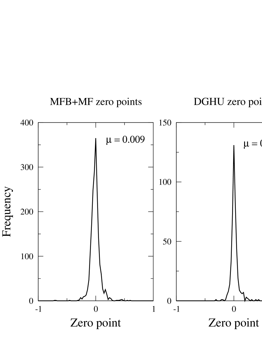
Figure 12: Plot of zero point for 1951 MFB+MF galaxies and 454 DGHU galaxies

9.3 Implications 1: The classical Tully-Fisher relation

9.3.1 Case $\Gamma=0$: Retrieval of the standard formulation

We begin by noting that a rearrangement of the second equation of (12), converting $\ln V_{0}$ to $\log\,V_{0}$, and setting $\Gamma=0$ gives

$$M\,=\,-7.29\,\log V_{0}\,-\,5.05.$$ (13)

Interpreting the characteristic scaling velocity $V_{0}$ as the disc ‘rotation velocity’, we can immediately recognize this relation as similar to a typical $I$-band Tully-Fisher calibration - but with a gradient on the low side. However, this latter relation was derived by combining two samples having different linewidth characteristics to make a specific point about the general analysis. Consequently, we might expect to find more typical gradients by analysing the four samples individually. In fact, we find:

$$M_{I}\, = \,-7.72\,\log V_{0}\,-\,3.79$$

$$M_{I}\, = \,-7.85\,\log V_{0}\,-\,3.54$$

$$M_{I}\, = \,-7.86\,\log V_{0}\,-\,3.71$$

$$M_{R}\, = \,-6.56\,\log V_{0}\,-\,6.48$$

respectively for the Mathewson et al Mathewson1992 (1992), Mathewson & Ford Mathewson1996 (1996), Dale et al Dale1997 (1997) and Courteau Courteau (1997) samples - the latter using Courteau’s $V_{max}$ linewidth definition as an example. We see that the three $I$-band gradients are now perfectly typical $I$-band TF gradients, whilst the single $R$-band gradient is now a perfectly typical $R$-band TF gradient. Similarly, for each case, the zero points are typical for $H\approx 85\,$km/sec/Mpc. We can therefore reasonably conclude that the second equation of (12) with $\Gamma=0$ recovers the standard formulation of the Tully-Fisher relation.

It now follows directly that the third equation of (12), for the characteristic scaling radius $R_{0}$, effectively defines the position on an ORC at which the rotation velocity, $V_{0}$, is to be measured. That is, for the example given, the $\Gamma=0$ case corresponds to measuring a characteristic rotation velocity $\ln V_{0}=-1.596-0.316\,M$ at a characteristic radial position $\ln R_{0}=-7.614\,-0.474\,M-0.0050\,S$.

9.3.2 Case $\Gamma\neq 0$: Arbitrariness in calibration procedures for TF

Given the $\Gamma=0$ case, it is now easy to see that the $\Gamma\neq 0$ case corresponds to measuring a characteristic rotation velocity, $V\equiv\exp(\Gamma)\,V_{0}$, at the radial position $R\equiv\exp(\Gamma/\alpha)\,R_{0}$. Thus, according to the present considerations, there is an arbitrariness in calibrating Tully-Fisher relations which consists in the freedom to choose which point on an ORC to use as the characteristic radius for the measurement of the characteristic rotation velocity. Also, since $\Gamma$ is an arbitrary function - and not just a constant - this freedom of choice can extend to, for example, a procedure whereby the place at which the rotation velocity is defined can be luminosity dependent.

This has significant consequences since, as mentioned in §B.2, there are several non-equivalent heuristically defined methods which authors use to estimate optical linewidths and there is, as yet, no concensus about which method is ‘best’. But, according to the above comments, it is clear that the ‘best’ such method is the one which most consistently selects the radial positions $R\equiv\exp(\Gamma/\alpha)\,R_{0}$ across the sample under consideration, for some $\Gamma$.

9.4 Implications 2: Non-classical Tully-Fisher formulations

The foregoing considerations give rise to distinct Tully-Fisher formulations neither of which is logically prior to the other. They are equivalent in the sense of being equally applicable to the problem of scaling.

9.4.1 The quasi-classical formulation

If we choose the $\Gamma=0$ calibration, then (12) can be expressed as:

$$\ln V_{0} = -1.596-0.316\,M$$

$$\ln R_{0} = -(1.596+0.316\,M+\ln A_{i})/\alpha\,$$ (14)

$$i = 1,2,3,4.$$

As we saw in §9.3.1, the first of these equations provides a typical $I$-band Tully-Fisher calibration whilst the second effectively says where on an ORC the linewidth, $V_{0}$, is to be measured. Note that, in this formulation, $\ln V_{0}$ varies only with $M$ as in any conventional Tully-Fisher calibration, but $R_{0}$ varies with $M$ and the dynamically measured quantities $(\alpha,\,\ln A)$.

9.4.2 The non-classical formulation

Equivalently, with the same $\Gamma=0$ calibration, (12) can be expressed as

$$\ln V_{0} = -\alpha\,(7.338\,+0.461\,M+0.00449\,S)+\ln A_{i}$$

$$i = 1,2,3,4$$

$$\ln R_{0} = -(7.338\,+0.461\,M+0.00449\,S).$$

In this formulation, we see that the classical situation is reversed. Now $\ln V_{0}$ varies with $M$ and the dynamically measured quantities $(\alpha,\,\ln A)$. Consequently, unlike in the classical formulation, both gradient and zero point will vary across the luminosity/dynamical range of a sample. By contrast, it is $R_{0}$ which varies with just luminosity properties, $M$ and $S$.

9.5 Comments on general calibration procedures

For the sake of explicitness, we shall use (14) to outline a suggested algorithmic approach to the calibration procedure for a sufficiently large sample. The approach is non-trivial and has yet to be developed into a fully working method:

1. Use the model (14), or something similar, as first guess at the final calibration;

2. Fold an unscaled ORC and determine its $\alpha$ - which is a scale-independent quantity;

3. Estimate which $\ln A_{i}$ is appropriate for the ORC using the $(\alpha:\ln A)$ correlations implicit in figure 11;

4. Iterate on the two equations of (14) and the power-law $V=A\,R^{\alpha}$ fitted to the ORC, to find $(R_{0},V_{0},M)$ for the galaxy concerned. The individual ORC can now be scaled;

5. Complete steps 2,3 and 4 for the whole sample and then:

   1. calculate the new $\ln A$ frequency diagram and compare with some template distribution such as that of figure 2;

   2. check if the calibration which comes out of the model (in the manner of (11)) is the same as the model which went in at step 1 - to within tolerance;

   If both these tests are satisfied, then accept the current calibration. If not, adjust the calibration, and repeat steps 2, 3, 4 and 5 until converged.

10 Major Stability issues

Apart from the importance of good Tully-Fisher calibrations and linewidth determinations, the successful extraction of the discrete dynamical states phenomonology from ORC data is also critically dependent on the quality of the folding process and the algorithmic computation of $\ln A$. We consider these in turn.

10.1 The quality of folding

In the literature, the folding of ORCs is most commonly described in the context of estimating linewidths for TF applications and, in such circumstances, the folding process generally amounts to determining an estimate of $V_{sys}$, the velocity equivalent of the systematic redshift. So far as we are aware, Persic & Salucci Persic1995 (1995) were the first to address the idea that ORCs folded for TF purposes were not necessarily folded with sufficient accuracy for the purpose of studying the interior dynamics of galaxy discs. It was for this reason that they provided their own folding solutions for the Mathewson et al Mathewson1992 (1992) sample. Possibly their main innovations to the folding process were, firstly relaxing the assumption that the dynamic centre of a spiral coincided with its optical centre. Hence, their folding process became a two-parameter problem - to determine $V_{sys}$ and the angular offset between the dynamical and optical centres, $\Delta\Phi$ say. Secondly, they introduced the pre-folding data filtering technique described in §3.1 which has the effect of discarding, typically, the least accurate 40% of velocity determinations on an given ORC. They then applied a labour-intensive ‘by-eye’ approach to the folding problem. The folding algorithm developed for the present study (Roscoe 1999c ) followed Persic & Salucci in utilizing both of these refinements.

To illustrate the effect of folding without these refinements, figure 13 shows the $\ln A$ frequency diagram computed for the Mathewson et al sample Mathewson1992 (1992), but using Mathewson et al’s own folding solution. This is to be compared directly with figures 1 and 2. It is quite clear that the discrete states phenomonology is heavily obscured in figure 13.

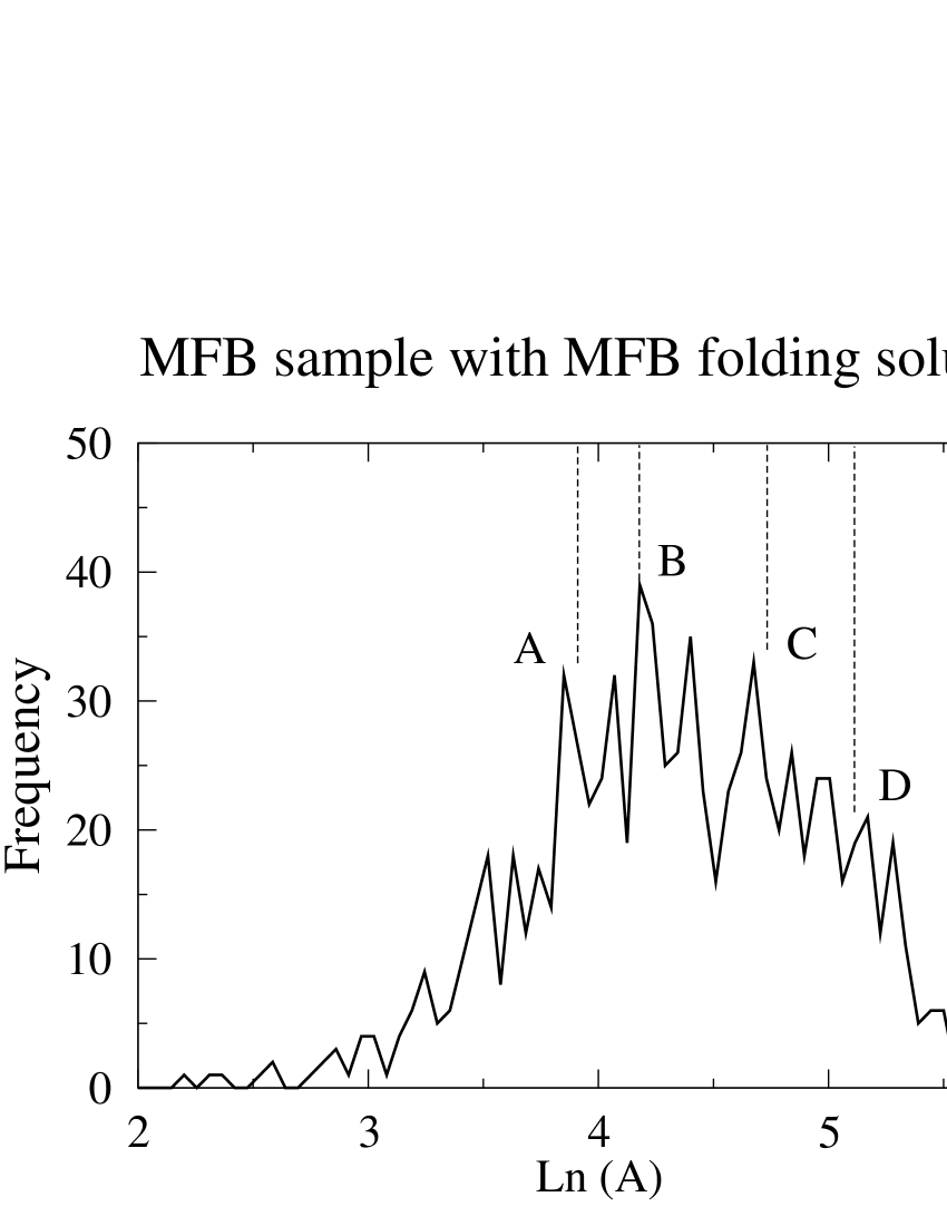
Figure 13: $\ln A$ distribution for the Mathewson et al Mathewson1992 (1992) sample with MFB folding and original Mathewson et al TF scaling; Vertical dotted lines indicate peak centres of Persic & Salucci solution. Bin width = 0.055

10.2 The quality of $\ln A$ determinations

The quality of $\ln A$ determinations is equally critical to the extraction of the discrete states phenomonology. Specifically, $\ln A$ is computed according to the ‘black-box’ algorithm of §3.3 which has the effect of, on average, discarding approximately the inner 10% of any given ORC. The value of $\ln A$ is then computed directly on the remaining outer segment of the ORC.

The typical consequences of not using this algorithm, and computing $\ln A$ on the whole ORC, are shown in figure 14 which gives the $\ln A$ frequency diagram arising from the Mathewson et al Mathewson1992 (1992) sample after it has been folded using our autofolder technique but without using the computational method of §3.3. Again, we see that the discrete states phenomonology is completely obscured.

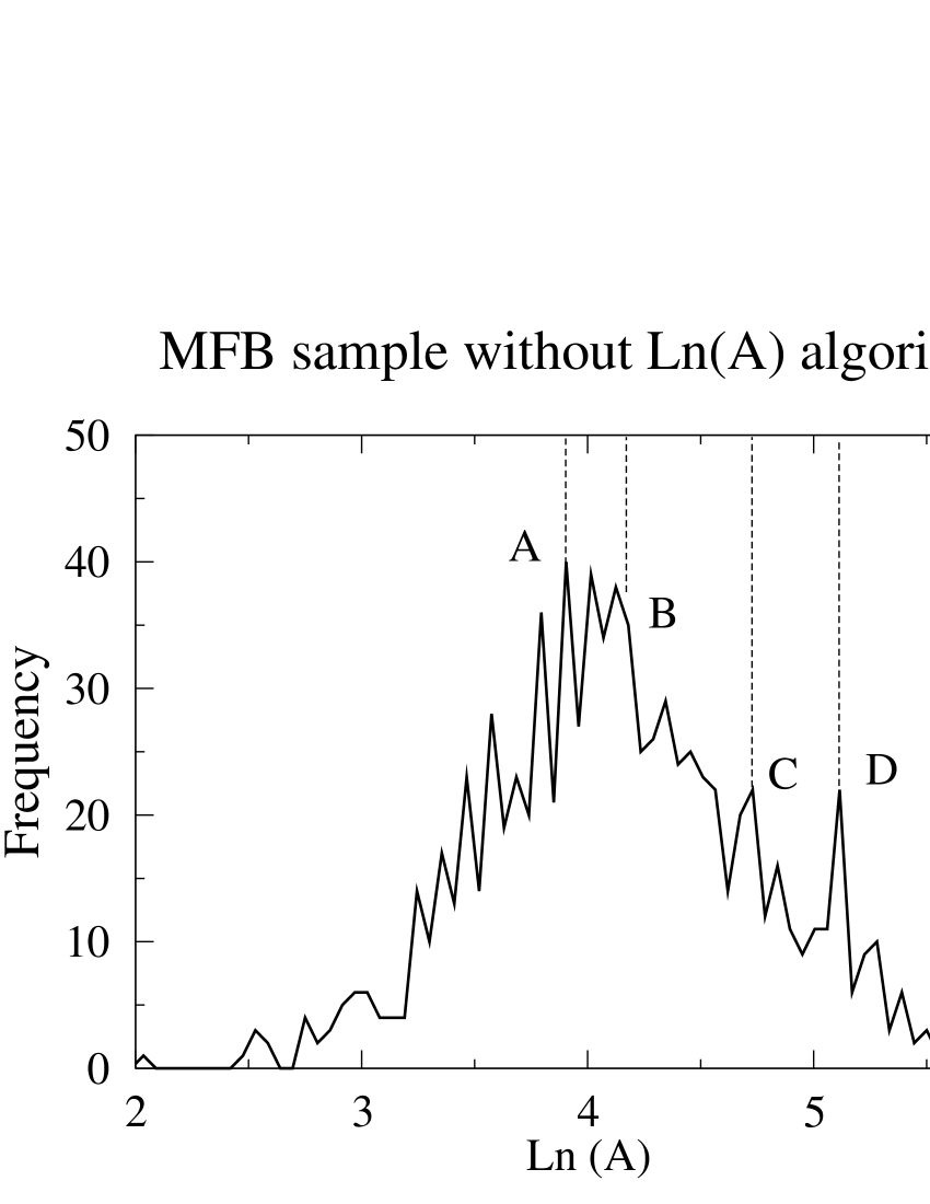
Figure 14: $\ln A$ distribution for the Mathewson et al Mathewson1992 (1992) sample with auto-folding and original Mathewson et al TF scaling, but without using the $\ln A$ algorithm; Vertical dotted lines indicate peak centres of Persic & Salucci solution. Bin width = 0.055

10.3 Effect of folding refinements on zero-point determinations for scaled ORCs

It is of interest to consider the zero-point distribution arising from regressing the scaled velocities, $\ln(V/V_{0})$ on the scaled radial coordinates, $\ln(R/R_{0})$, when the $(R_{0},\,V_{0})$ model is obtained from ORCs folded using simply $V_{sys}$ determinations and without applying the $\ln A$ algorithm of §3.3. To illustrate the point, the right panel of figure 15 show the distribution arising from the combined Mathewson et al Mathewson1992 (1992) and Mathewson & Ford Mathewson1996 (1996) samples using their original folding solutions, and without using the $\ln A$ algorithm. The left panel, included for comparison, arises from the same combined sample, but with our various folding refinements included.

It is obvious from the figure that the effect of using the original folding solutions and omitting our refinements is simply to add unbiased noise to the zero-point solutions. However, it is interesting to note that, even when the original folding solutions are used and our various refinements are omitted, the zero-point frequency distribution still provides strong support for the power-law description of ORCs.

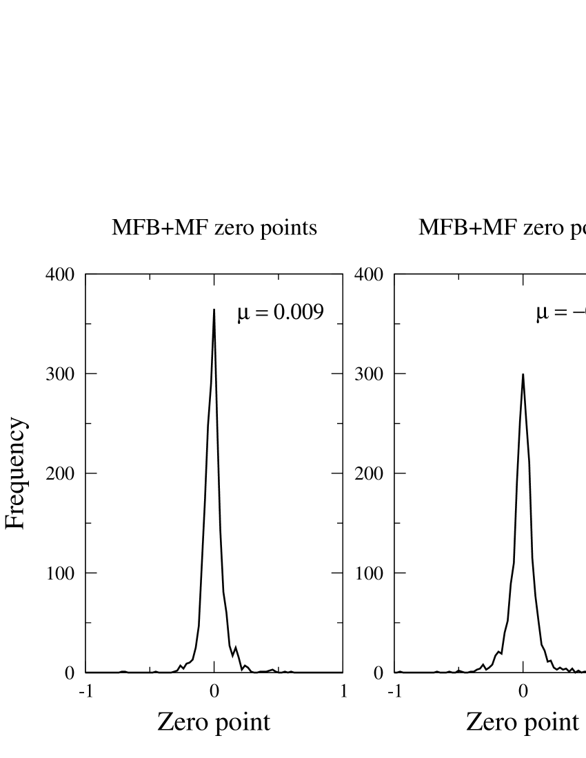
Figure 15: Left panel: zero-point distribution arising from mfb+mf combined sample of scaled ORCs with auto-folder and $\ln A$ algorithm. Right panel: similar to left panel, but with Mathewson’s original folding solution and no $\ln A$ algorithm. Bin width = 0.055

11 General dynamical implications

The present analysis has allowed us to established to a very high degree of statistical certainty that the parameter $\ln A$ appears constrained to take on discrete values $k_{1},k_{2},...$. Combining this with, say, (11) which showed $\ln A\approx F(M,\,S,\,\alpha)$, then we must have $F(M,\,S,\,\alpha)=k_{1},k_{2},...$. Thus it appears that spiral galaxies are constrained to exist on one of a set of discrete class planes in the three-dimensional $(M,S,\alpha)$ space. This then gives rise to one of two broad possibilities: at some stage in its evolution a spiral galaxy somehow moves onto one of these discrete class planes and then:

• is either necessarily constrained to remain on this plane over the whole of its evolution;

• or has the possibility of transiting to other planes in very short periods of time, so that the planes themselves represent an evolutionary sequence.

In either case, the primary difficulty is identifying mechanisms which might generate such discrete sets of possible dynamical class planes and, in the following, we make three conjectures.

11.1 First conjecture

In the wider world on non-linear dynamical systems, it is not difficult to find (or to construct) systems for which consistent solutions can only be found when certain algebraic conditions are satisfied - not eigenvalue problems, but analogous to them. If, in such a system, the algebraic condition had the form of a quartic defined in the system’s parameter space then, immediately, one would have a situation in which the solutions fell into four discrete dynamical classes. Our first conjecture is, therefore, that disc dynamics are governed by just such a non-linear system so that the discrete dynamical class phenomonology is merely a manifestation of an unknown algebraic consistency condition.

11.2 Second conjecture

Within the context of inflationary cosmologies, scalar fields play a critical role in the early universe. Since it is not difficult to induce oscillatory behaviour in these scalar fields, it becomes natural to consider the possibility that the four dynamical classes of our analysis are the frozen imprint of four distinct galaxy-formation epochs in the early universe, each associated with a distinct oscillation of the scalar field. If this is the case, then the phenomonology provides a very strong constraint on these early galaxy formation processes.

11.3 Third conjecture

Until recently, the most popular candidate for constituting the dark matter that is required to produce the generality of observed rotation curve shapes (especially for the dimmer galaxies, and beyond optical limits in general) has been the neutralino. However, this conjecture is now in serious difficulties since simulations show that these massive particles would tend to accumulate in large agglomerations which would cause serious disruption of galactic structure which is not observed. In response to this state of affairs, Arbey et al Arbey (2001) have proposed the existence of a massive non-self interacting charged scalar field as an alternative source of ‘dark-matter’ action. They provide a fairly comprehensive analysis to show how their conjecture provides extremely good fits to the six brightest of Persic et al’s Persic1996 (1996) eleven classes of universal rotation curves.

More particularly, from our point of view, the conjectured dark halo of Arbey et al Arbey (2001) is based on a primitive ‘boson star’ model, and this model is constrained so that it gives rise to a sequence of discrete energy eigenstates, each of which is associated with distinct measures of rotation for the ‘boson star’. Whilst it is true that these discrete rotation states do not correspond in any direct way to the discrete dynamical classes discussed in this paper, it must be considered remarkable that such a prediction arises at all in a paper which was primarily directed towards attempting to model the universal ORCs of Persic et al Persic1996 (1996). It seems, therefore, that the phenomonology discussed here may potentially be understood in terms of the quitessential galactic haloe.

12 Summary and Conclusions

We have analysed four separate large ORC samples to show that the discrete dynamical classes hypothesis for galaxy discs is supported by the data at the level of virtual certainty. The immediate significance of the phenomonology is that any given spiral galaxy appears to be constrained to evolve over one of a discretely defined set of dynamical class planes, existing in a three-dimensional $(M,S,\alpha)$ space where $M$ is absolute magnitude, $S$ is surface brightness and $\alpha$ is a parameter computed for each galaxy from its rotation curve.

We have shown how the broader analysis implies the existence of a second generation of Tully-Fisher methods which augment the classical Tully-Fisher relationship with a second, similar, relationship which defines where on an ORC the linewidth is to be measured. An algorithm for the absolute calibration of this extended Tully-Fisher method was then proposed.

We have conjectured three possible mechanism for this phenomonology, one based on the idea that the phenomonology is the manifestation of an algebraic consistency condition in some (unkown) non-linear dynamical system theory which describes disc dynamics, a second based on the notion of a sequence of distinct galaxy-formation epochs in an oscillating early universe, and a third based on the dynamical effects of quintessential halos acting as the source of dark matter around spirals.

Whatever the truth of the matter, it seems certain that the existence of the distinct dynamical classes poses very difficult questions for the standard galaxy formation theories, and will have a a potentially profound affect on our developing understanding of galactic dynamics and evolution in particular, and the cosmos in general.

Acknowledgements

I am grateful to M. Persic and P. Salucci, of SISSA Italy, D. Mathewson (now retired) and V. Ford of Mt Stromlo Observatory ANU, D. Dale of the California Institute of Technology, R. Giovanelli & M. Haynes of Cornell University and S. Courteau of the Herzberg Institute of Astrophysics Canada, for making available their data, and for patiently answering all queries, and to Bill Napier of Armagh Observatory, UK, for many fruitful discussions during the course of this work.

Appendix A The Effects of Tully-Fisher Scatter on $\ln A$ Profiles

All the distance scaling in this analysis is performed using Tully-Fisher methods, which possess well-understood inherent sources of error. Consequently, we need to understand the extent to which these errors can affect the phenomenon which is the subject of the present analysis.

Mathewson et al Mathewson1992 (1992) report a magnitude scatter of about 0.32 for their sample (our best) which compares favourably with that of 0.35 reported by Courteau for his sample. These correspond to a scatter of less than 20% for distance measurements and, in the following, we analyse the effects of such uncertainties on our proposed analysis to demonstrate that they cannot wash out any potential peak structures of the type seen in figure 1.

Suppose that each galaxy in the sample has had its distance exactly determined, and that $R$ denotes the corresponding exact radial scale. Then $V=AR^{\alpha}$ implies

$$\ln V=\ln A+\alpha\ln R.$$

The existence of uncertainties in the Tully-Fisher distance scale with a typical scatter of 20% can be accounted for by the replacement $R\rightarrow kR$ where $0.8\leq k\leq 1.2$, so that

$$\ln V=\ln A+\alpha\ln k+\alpha\ln R\equiv\ln A^{\prime}+\alpha\ln R,$$

where $\ln A^{\prime}\equiv\ln A+\alpha\ln k$. We immediately see that uncertainties in the distance scale affect the zero point in the $(\ln R,\ln V)$ relationship, but leave the gradient $\alpha$ unaffected.

Since $0.8\leq k\leq 1.2$ then, as an approximation, $-0.2<\ln k<0.2$ so that $\ln A^{\prime}\equiv\ln A\pm 0.2\alpha$. The peak structures of figure 1 lie in the approximate range $3.9<\ln A<5.1$ (that is, $1.7<\log A<2.2$) and reference to Roscoe 1999b (figure 8) shows that this corresponds to the approximate range $0.18<\alpha<0.55$, where low $\alpha$ corresponds to the brightest galaxies and vice versa. Therefore, for the brightest galaxies, we have $\ln A^{\prime}\equiv\ln A\pm 0.04$ whilst, for the dimmest galaxies, we have $\ln A^{\prime}\equiv\ln A\pm 0.1$. That is, uncertainties of 20% in the Tully-Fisher distance scale create uncertainties in $\ln A$ of $\pm 0.04$ at the bright end, and of $\pm 0.1$ at the dim end.

It follows that, since the mean separation of the $\ln A$ peaks in figure 1 is about 0.4, these uncertainties in the Tully-Fisher distance scale are incapable of washing out the discrete peak structure observed in the $\ln A$ distribution. This analysis provides the confidence required to analysise further samples on the same basis.

Appendix B The elimination of artifact as a mechanism

It is necessary to be as certain as is possible that the phenomonology being claimed is not created as an artifact of any particular procedure or data sample. There are three independent routes by which such an artifact (no matter how remote the possibility) could infiltrate the process, and these can be listed as:

• the original process of measuring ORCs;

• the method of linewidth estimation;

• the folding process.

B.1 The original measuring process

The possibility that an artifact can enter via the ORC measurement process is minimized by the fact that we analyse four different samples originating with three distinct groups of astronomers using three different telescopes in different hemispheres. A detailed discussion of the samples is given in §2.

B.2 Linewidth determinations

The possibility that an artifact can enter via the linewidth estimation process is minimized by the fact that five different methods of linewidth determination are employed over our four samples:

• The Mathewson et al Mathewson1992 (1992) sample has linewidths determined using a non-algorithmic and intuitive ‘eye-ball’ method (private communication);

• the Mathewson & Ford Mathewson1996 (1996) sample is considered using (a) Mathewson’s own ‘eye-ball’ linewidth determinations and (b) algortihmically determined linewidths based on $V_{opt}$, the velocity at the optical radius as defined by Persic & Salucci Persic1995 (1995);

• the Dale et al Dale1997 (1997) sample has linewidths determined by an elaborate process based on the $V_{90\%}-V_{10\%}$ linewidth estimator, which is similar to the technique first introduced by Dressler & Faber Dressler (1990);

• the Courteau sample was taken from the study of Courteau Courteau (1997) which was explicitly designed as a study of objective black-box methods of optical linewidth estimation. He tests a variety of methods, and we present results using those two which he judges to be the best, $V_{2.2}$, and the worst, $V_{max}$, respectively.

B.3 The folding process

Finally, the possibility that an artifact can enter via the folding process is minimized by the fact that the phenomenon is observed when either of two quite distinct folding methods is used. These two methods, described below, share the features introduced by Persic & Salucci Persic1995 (1995) that (a) the folding process requires the determination of two parameters, the primary one being $V_{sys}$ the systematic velocity (which is usually the only one considered), and the secondary one being $\Delta\Phi$ which measures the angular offset between the optical and the kinematic centres and (b) the pre-folding data filter described in §3.1. These features are considered necessary for the purpose of maximising folding accuracy.

B.3.1 The method of Persic and Salucci

Persic & Salucci Persic1995 (1995) were primarily interested in using rotation curves for studies of the interior dynamics of spiral galaxies and so, by their own criteria, had a requirement for a large sample of particularly accurately folded ORCs. They took the 965 ORCs of Mathewson et al Mathewson1992 (1992) and used an eye-ball method of folding to produce a sample of 900 good-to-excellent quality folded ORCs; as a qualitative measure of the effort expended to produce this sample, we can note that it took these two authors about a year to process it (private communication). Every velocity measurement in the Mathewson et al Mathewson1992 (1992) sample came provided with a parameter (varying on the range $(0,\,1)$) which estimated the relative internal accuracy associated with the measurement. Persic & Salucci Persic1995 (1995) found that the accurate folding of any given ORC required the rejection of any individual velocity measurement for which the associated accuracy parameter was $\leq\,0.35$. In the present context, only the Mathewson et al Mathewson1992 (1992) sample has been folded with this method.

B.3.2 The auto-folder method of Roscoe 1999c

This method was developed in anticipation of the need accurately to fold the Mathewson & Ford Mathewson1996 (1996) sample of 1200+ ORCs on a reasonable time-scale. The details of this method are described in Roscoe 1999c but, briefly, it is based on the formal minimization of the symmetric components in Fourier representations of ORCs with respect to variations in the two folding parameters.

The folding method was developed on that subset of the Mathewson et al Mathewson1992 (1992) sample used by Persic & Salucci Persic1995 (1995) and, corresponding to the experience of these latter authors, we found that the optimal trade-off point between the quality of individual velocity measurements, and the volume of good-quality data available for the automatic folding method, required the prior rejection of any individual velocity measurement which had an associated relative accuracy parameter $\leq\,0.4$. This is roughly equivalent to the requirement that the absolute error of any given velocity measurement should be $\leq\,5\%$.

This folding method has been used here on the samples of Mathewson et al Mathewson1992 (1992), Mathewson & Ford Mathewson1996 (1996), Dale et al Dale1997 (1997) et seq and Courteau Courteau (1997).

Appendix C Overview of the ORC dynamical partitioning process

We discuss two methods of assessing the efficiency and effectiveness of the process described in §3.3 for the computation of $\ln A$ and establish, with virtual certainty, the truth of the statements that:

• the innermost parts of ORCs exhibit behaviour which is qualitatively sharply distinguished from that exhibited by the outermost parts of ORCs;

• the size of such innermost sections can be quantified in terms of a radial measure, $R_{min}$ say, which can be shown to be extremely powerfully correlated with the independently defined optical radius, $R_{opt}$ (here, as given by Persic & Salucci Persic1995 (1995) of the disc. Since $R_{opt}$ carries physical information about the system, then we must conclude that the algorithmically estimated $R_{min}$ likewise carries physical information about the system. Given the quality of the statistics involved, these two points are entirely sufficient to establish that $R_{min}$ does, in fact, define a real boundary between distinct dynamical regimes which, in turn, gives a concrete justification to the technique by which it is estimated. We suggest that $R_{min}$ could act as a tracer for the gravitational radius of the core on the basis of the circumstance that there appears to be no other possible interpretation.

h

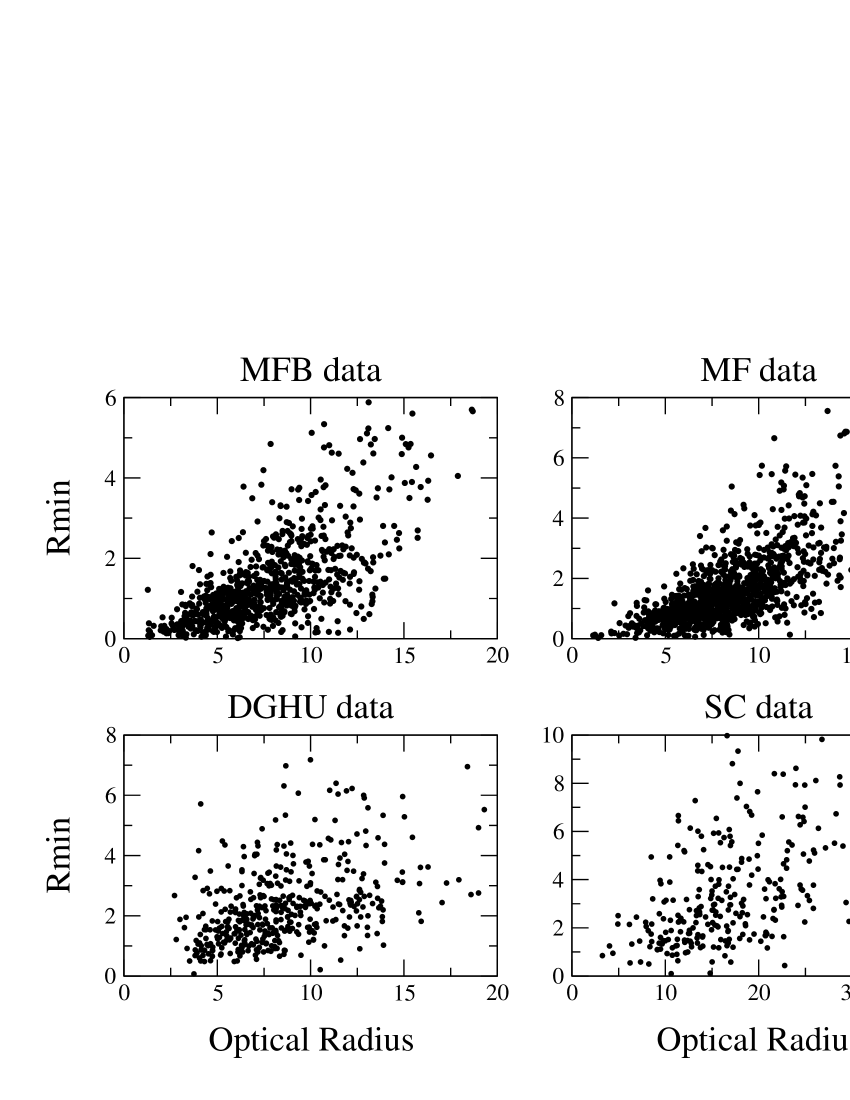
Figure 16: Scatter plot of $R_{opt}:R_{min}$ for MFB, MF, DGHU and SC data with dynamical partitioning

C.1 The first test of dynamical partitioning

We argued in Roscoe 1999b that, if $R_{min}$ really was a tracer for the gravitational radius of the core, then we might expect to find a positive correlation between $R_{min}$ and $R_{opt}$ - on the grounds that galaxies with large cores might be expected to have large optical radii etc.

The top-left panel of figure 16 shows the ($R_{opt}:R_{min}$) scatter plot for Mathewson et al data Mathewson1992 (1992), and we note the existence of an extremely strong positive ($R_{opt}:R_{min}$) correlation. The top-right panel shows an equally strong effect for Mathewson & Ford Mathewson1996 (1996) data, whilst the bottom-left panel shows a similarly strong effect for the Dale et al Dale1997 (1997) et seq sample, and and the bottom-right panel shows the same effect for the much smaller Courteau sample. The statistics underlying these diagrams are given in the various columns of table 9 and these confirm in quantitative terms what is obvious in the diagrams. We can therefore conclude with certainty that, since $R_{opt}$ is an objectively defined physical boundary, the $R_{min}$ is similarly an objectively defined physical boundary. We speculate that, in fact, it is a noisy tracer of the boundary between core-dominated and disc-dominated dynamics in the disc.

Table 9: $R_{opt}=b_{0}+b_{1}\,R_{min}$

	MFB		MF		DGHU		SC
Predictor	Coeff	t-ratio	Coeff	t-ratio	Coeff	t-ratio	Coeff	t-ratio
$Const.$	5.26	44	5.95	55	5.97	23	12.45	25
$R_{min}$	1.74	28	1.54	30	1.06	11	1.21	12
	$R^{2}$  =  48.9%		$R^{2}$  =  45.7%		$R^{2}$  =  22.2%		$R^{2}$ =  35.5%

The foregoing considerations lead to the following conclusions:

• The application of the dynamical partitioning process produces a very powerful, although noisy, $R_{min}:R_{opt}$ correlation confirming that $R_{min}$ (as computed by dynamical partitioning) is a strong tracer for $R_{opt}$;

• The computed value of $R_{min}$ defines a physical transition boundary between core-dominated dynamics and disc-dominated dynamics.

Taking these items together, and noting the absence of any other obvious interpretation, we conclude that $R_{min}$ almost certainly represents a dynamically derived tracer of the gravitational radius of the core.

Table 10: Effect of dynamical partitioning technique on power-law fits

Dynamical	MFB	MF	DGHU	SC
partitioning	Mean rms	Mean rms	Mean rms	Mean rms
Before	$10.8\times 10^{-2}$	$12.0\times 10^{-2}$	$1.1\times 10^{-2}$	$1.8\times 10^{-2}$
After	$\leavevmode\nobreak\ 2.4\times 10^{-2}$	$\leavevmode\nobreak\ 3.4\times 10^{-2}$	$0.6\times 10^{-2}$	$1.4\times 10^{-2}$
Statistics calculated on the 866 ORCs of MFB, the 1085 ORCs of MF
the 454 ORCs of DGHU and the 283 ORCs of SC.

C.2 The second test of dynamical partitioning

The second definitive formal measure of the statistical efficiency of dynamical partitioning is given in table 10. The first row of this table gives the averaged root mean square (rms) error calculated from fitting power-laws to each of the 866 foldable ORCs of the Mathewson et al Mathewson1992 (1992) sample, the 1085 foldable ORCs of the Mathewson & Ford Mathewson1996 (1996) sample, the 454 foldable ORCs of the Dale et al Dale1997 (1997) et seq sample and the 283 foldable ORCs of the Courteau Courteau (1997) sample before the dynamical partitioning process. The second row gives the corresponding averaged rms values after the dynamical partitioning process. Column 2 refers to Mathewson et al Mathewson1992 (1992) data, column 3 refers to Mathewson & Ford Mathewson1996 (1996) data, coulumn 4 refers to Dale et al Dale1997 (1997) et seq data and column 5 refers to Courteau Courteau (1997) data. The Mathewson et al Mathewson1992 (1992) data shows an almost 80% reduction in its mean rms, the Mathewson & Ford Mathewson1996 (1996) data shows a 72% reduction in its mean rms, the Dale et al Dale1997 (1997) et seq data shows a 45% reduction in its mean rms and the Courteau Courteau (1997) data shows a 29% reduction in its mean rms.

Since the dynamical partitioning process leads to the discarding of only 12% of the Mathewson et al Mathewson1992 (1992) and the Mathewson & Ford Mathewson1996 (1996) data (out of a total of about 37000 individual measurements over the two samples), of only 9% of the Dale et al Dale1997 (1997) et seq data (out of a total of 15000 individual measurements) and of only 10% of the Courteau Courteau (1997) data (out of a total of about 17000 individual measurements), then we can categorically state that the table provides conclusive evidence for the statement that the deviation from the power-law fit is strongly concentrated on the inner 10% or so of ORCs. From this we can conclude that the behaviour of the inner 10% or so of ORCs is qualitatively sharply distinguished from the outer 90% or so, as we would expect on purely dynamical grounds.

Appendix D Confidence limits on peak positions

We use bootstrap techniques to show that the uncertainties in the positions of the $A,\,B,\,C,\,D$ peaks of figure 2, are small. The process adopted is described as follows:

• Partition the range of $\ln A$ into the sub-ranges $(2.200,4.070)$ containing peak $A$, $(4.070,4.455)$ containing peak $B$, $(4.455,4.950)$ containing peak $C$ and $(4.950,6.000)$ containing peak $D$;

• Use the actual $\ln A$ data-set of $N$ distinct $\ln A$ values to generate 1000 bootstrapped simulated data-sets, each consisting of $N$ values generated by random selection from the real data-set with replacement;

• Form the frequency diagram for each of the 1000 simulated data-sets, and record the position of the largest signal only in each of the four sub-ranges defined above;

• Form the frequency diagram for this ‘largest signal’ data set - this is plotted in figure 17.

We now discuss the peaks in figure 17 in turn: Peak $A$: $\ln A=3.91$ This peak coincides exactly with peak $A$ of figure 2. Since $\ln A$ correlates in a strong positive sense with absolute luminosity (Roscoe 1999b , then this peak corresponds to the dimmest end of the sample, so that greater measurement uncertainties probably account for the relative broadness of this peak; even so, this peak is still very tightly defined and the 90% confidence interval this peak is (3.87,3.98). Peak $B$: $\ln A=4.18$ This peak coincides exactly with peak $B$ of figure 2 and is the most straightforward case, being very tightly defined with no subsidiary peaklets; in fact, more than 97% of the sampled $B$ peaks fall in a single bin, so that we can assert that an extremely conservative 90% confidence interval for this peak is given by the bin boundaries as (4.15,4.21). Peak $C$: $\ln A=4.73$ This peak exhibits a bi-modal structure with the major mode coinciding exactly with the peak $C$ of figure 2; the minor peak contains about 10% of the sampled $C$ peaks, with the remainder being in the major peak. The boundaries of the major peak, given by (4.70,4.76), therefore give an estimate of a 90% confidence interval for the $C$ peak. Peak $D$: $\ln A=5.12$ Again there is a bi-model structure, but this time the minor mode is very much more prominent than it is for the $C$ peak. We find that the minor peak contains approximately 20% of the sampled $D$ peaks, with the remainder being in the major peak. To simplify the complexities presented by this bi-modal structure, we simply choose the boundaries of the major peak as estimates of the required 90% confidence interval for the $D$ peak.

Figure 17: Frequency diagram for the positions of the largest signals near the original $A,B,C,D$ peaks, bootstrapped from the MFB sample over 1000 trials

References

- (1) Arbey, A., Lesgourgues, J., Salati, P., 2001, Astro-ph/0105564 V2,
- (2) Bosma et al. 1992, ApJ 400, L21-24
- (3) Courteau S., 1997, AJ, 114, 6, 2402-2427
- (4) Dale DA, Giovanelli R, Haynes M, 1997 AJ 114 (2): 455-473
- (5) Dale DA, Giovanelli R, Haynes MP, Scodeggio M, Hardy E, Campusano LE, 1998 AJ 115 (2), 418-435
- (6) Dale D.A., Giovanelli R, Haynes M.P., 1999, AJ 118 (4), 1468-1488
- (7) Dale D.A., Uson JM, 2000, AJ 120 (2), 552-561
- (8) Dale D.A., Giovanelli R, Haynes M.P., Hardy E, Campusano LE, 2001, AJ 121, 1886-1892
- (9) Dressler A., Faber S.M., 1990, ApJ, 345, 45
- (10) Giovanelli R., Haynes M.P., Herter T., Vogt N.P., da Costa L.N., Freudling W., Salzer J.J., Wegner G. 1997 AJ 113 (1), 53
- (11) Lynden-Bell D., Lahav, O., Burstein, D., 1989, MNRAS, 241, 325
- (12) Mathewson D.S., Ford V.L., Buchhorn M. 1992, ApJS 81 413
- (13) Mathewson D.S., Ford V.L. 1996, ApJS 107 97
- (14) Persic M., Salucci P., Stel F., 1996, MNRAS 281 27
- (15) Persic M., Salucci P., 1991, ApJ 368 60
- (16) Persic M., Salucci P., 1995, ApJS 99 501
- (17) Roscoe D.F., 1999a, A&A,343, 697-704
- (18) Roscoe D.F., 1999b, A&A,343, 788-800
- (19) Roscoe D.F., 1999c, A&AS,140, 247-260
- (20) Rubin V.C., Ford W.K., Thonnard N. 1980, ApJ 238 471