A possible use for polarizers in Imaging Atmospheric Cherenkov Telescopes

Abstract

Cherenkov radiation produced in Extensive Air Showers shows a net polarization. This article discusses its properties and physical origin, and proposes an arrangement of polarizers potentially useful for Imaging Atmospheric Cherenkov Telescopes.

, , ,

1 Introduction

The purpose of this work is twofold. For one, it studies a widely neglected aspect of Very High Energy (VHE) Extensive Atmospheric Air Showers (EAS), namely the polarization of the Cherenkov light. For another, it proposes an experimental setup that could be used to take advantage of the net polarization in EAS in the field of Imaging Atmospheric Cherenkov Telescopes (IACTs).

We shall proceed as follows. To begin with, the basic physical ideas that explain why a net polarization of the Cherenkov light is expected in an EAS will be outlined and some features of this polarization will be discussed. Section 3 will propose an experimental setup which exploits the net intrinsic polarization of showers initiated by $\gamma$-rays and in a lesser degree of those initiated by charged cosmic rays. A detailed study of the setup has been carried out using a Monte Carlo (MC) simulation that will be described in section 4. The result of this study is presented in section 5. A short discussion relevant to some related situations not considered in the paper has been left for section 6.

2 Physical basis

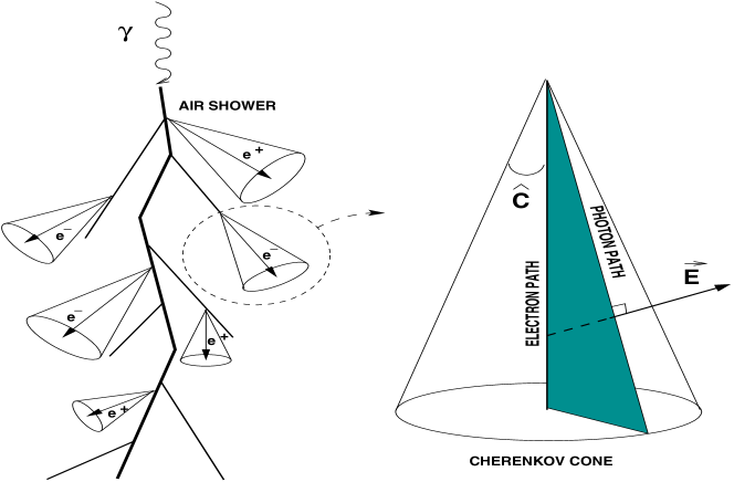
Figure 1: Top left: a schematic representation of an air shower illustrating single particle cherenkov cones. Top right: the polarization vector is contained in the plane defined by the electron path and the photon path and is perpendicular to the photon path. Bottom left, the coordinate system and polarization parameters as referred in the text are illustrated. Bottom right, polarization vector distribution on ground for a 1 TeV $\gamma$-induced MC event at three core distances. Each circle represents all the Cherenkov photons falling at that particular core distance.

The Cherenkov radiation emitted by a relativistic charged particle moving in a dense medium is distributed along a cone whose apex moves with the particle and whose axis is the particle path. The opening angle of the Cherenkov cone in the air is of the order of one degree. It is well known that Cherenkov radiation exhibits an intrinsic polarization [12, J. V. Jelley 1958]. The electric field vector of the emitted light is contained in the plane defined by the particle and photon paths (see Fig. 1 upper right).

The existence of a net linear polarization in the light produced by an EAS can be readily understood within a simple limiting case. Suppose a normally incident shower with respect to the ground, whose particles travel along the shower axis. The light pattern left on the ground by the shower particles would be a superposition of circles centered in the shower core, defined as the point where the shower axis touches ground. The polarization of the photons hitting the ground would always lie in the line passing through their point of impact on ground and the shower core.

To describe the depicted situation it is convenient to define a system of cylindrical coordinates, centered at the core, with the $Z$ axis directed upwards along the shower axis. In this frame the polarization of the Cherenkov photons lie in the $XY$ plane, in lines pointing to the core. The expression radial direction will often be used to mean the direction of these lines. While the polarization of the Cherenkov photons in a real shower does not always follow the radial direction, it falls to a good approximation on the $XY$ plane. Therefore the angle which they form with the radial direction is a good measure of their deviation from the limiting case described before. Hereafter it will be named $\theta_{pol}$.

A real shower is not expected to behave in a manner substantially different to the limit case described before. A net polarization in the radial direction can be expected when the distance of the incident point to the core is much larger than the distance of the emitting particle to the shower axis (i.e. when the shower is observed with less transverse angular spread) and the direction of the emitting particle is similar to the shower axis. Both conditions are satisfied in a wide range of situations, since the density of particles in an EAS is maximal at small angles and distances with respect to the shower core. Factors like the Coulomb scattering and the hadronic interactions are determinant to disperse the shower particles in angle and core distance and thus are expected to influence the degree of net polarization along the radial direction.

As an illustration Fig. 1, at the right bottom, shows the distribution of polarization vectors at three different core distances for a MC-generated shower initiated by a $\gamma$-ray.

Besides the above-discussed general considerations, the polarization of the Cherenkov light carries additional information about the EAS. This will be discussed in more detail in the following sections. The accompanying plots have been generated using a MC simulation whose setup is described in section 4. Throughout all the sections it will be assumed that incident $\gamma-ray$ showers are normal to the ground, i.e. the zenith angle is equal zero. This assumption is not as restrictive as it may seem, since the reflector of an IACT is always practically perpendicular to the shower axis, a situation in many ways equivalent to normal incidence.

In our simulation we have not considered the correlation between the degree of polarization and the wavelength of the incoming Cherenkov photons. Its study calls for a detailed model of the atmosphere and the polarizing filter. Nevertheless the different light attenuation in the atmosphere at different wavelengths must lead to a noticeable correlation between these two quantities. For instance, the observed ultraviolet light is mostly produced in the final stages of shower development since it is strongly attenuated in the atmosphere. It must therefore present a lower degree of polarization than light at other wavelengths. This could prove interesting for experiments operating at these wavelengths such as CLUE  [2, B. Bartoli 1998].

2.1 Dependence on the distance to the core and particle type

Showers initiated by $\gamma$s are closer to the aforementioned ideal shower than hadron-initiated showers.

The reason lies in the relatively large transverse momentum of the hadronic interactions compared with the purely electromagnetic interactions in gamma-ray showers. This results in a general spread in the shower particles. Therefore the net polarization along the radial direction is expected to be larger in $\gamma$ showers than in hadronic ones, as already noted by Hillas  [11, A. M. Hillas 1996]. Clear differences are seen in the radial distributions of both types of primary particles.

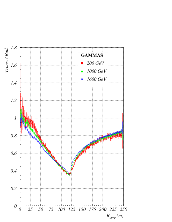
Figure 3: MC simulation of the polarization distribution at the ground for primary $\gamma$s of different energies. The distribution shown is the same as in figure 2 where each curve is a superposition of 10 showers.

At first sight, the general arguments discussed above seem to imply an increase of the degree of radial polarization with core distance r. The reason being that the region around the shower axis with significant particle density is observed under an always smaller angle as we move away from the shower core in the ground. However a detailed simulation shows that the degree of radial polarization is not a monotonically increasing function of r (as illustrated in Fig. 3). Whereas the polarization behaves as expected at r out to the so-called hump of the lateral distribution ($\sim$ 120 m), other factors, such as multiple scattering, reduce the degree of polarization at larger r. The result is a maximum in the lateral distribution of the degree of polarization.

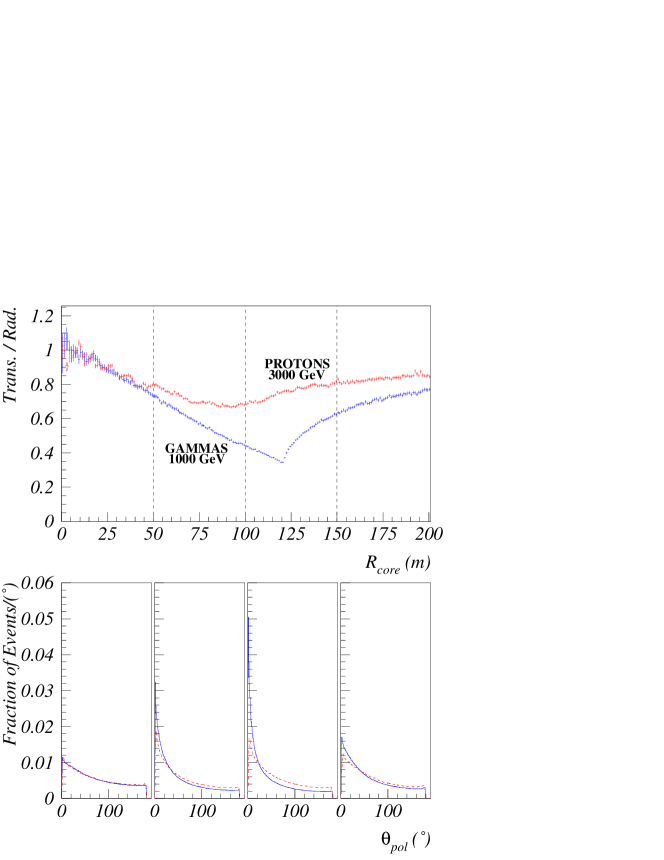
Figure 2: On the upper plot the transverse component over the radial component of the polarization vectors is represented as a function of the core distance for a superposition of 10 $\gamma$ MC events at 1 TeV and a superposition of 10 hadron MC events at 3 TeV within 3 degrees of zenith angle . On the lower plots the distribution of the angle $\theta_{pol}$ over four different core distance intervals, the ones indicated by the vertical dashed lines on the top plot, is shown. The dashed line on the bottom plots stands for protons.

The behavior of the degree of polarization with respect to r depends on the nature of the particle which gives origin to the EAS. Showers originated by Very High Energy $\gamma$-rays display a maximum around the hump of the Cherenkov lateral distribution. EAS of hadronic origin exhibit a not so abrupt turning point at shorter r (as can be seen in Fig. 2). The influence of the primary particle species was already noted by Hillas in  [11, A. M. Hillas 1996] and advanced as a $\gamma$/hadron discriminator.

In addition there is a small dependence with the energy of the primary particle (see Fig. 3). The position of the maximum is however energy independent.

Although no attempt has been made to understand in detail the difference with particle species, physical arguments point to the influence of multiple scattering as determinant of the position of the maximum, and transverse momentum to the difference between hadrons and $\gamma$s. In the case of $\gamma$ EAS, this belief is enforced by the fact that the maximum is reached near the hump, the point which would mark the edge of the Cherenkov pool if no multiple scattering was present. Other correlated factors, as the detailed shape of the transverse profile may also influence this result.

2.2 Dependence on emission point

The above-depicted limiting case (all particles moving along the shower axis) is closer to the trajectories of the particles in the first stages of a real shower development than in its later stages. The reason is that multiple scattering, and transverse momentum in the case of hadronic interactions, have not diffused the shower particles yet. As a result the Cherenkov light emitted by particles in the first stages of shower development shows a higher degree of polarization.

Fig. 4 shows the median of the $\theta_{pol}$ distribution, in a plane perpendicular to the shower axis, as a function of the atmospheric depth at which the Cherenkov photons have been produced. This median has been computed in bins of one radiation length. Horizontal bars represent the dispersion of the distribution of $\theta_{p}ol$, computed as the interval containing 68% of the distribution, half of it at each side of the median. To produce the plot, ten gamma and ten proton showers have been generated. The first interaction point has been fixed at 35 km. The figure shows how the median and the spread of $\theta_{pol}$ increase as the shower develops. It indicates a decrease of the degree of polarization along the radial direction with atmospheric depth, both for $\gamma$ and proton initiated EAS.

2.3 Correlation of polarization and time of arrival

There is also a strong correlation between the time of arrival of the Cherenkov photons at ground and the value of their radial polarization. For particles traveling along the shower axis it can be easily shown that light at a core distance r can only arise from a limited range of heights. Therefore the time of arrival of the photons is also expected to be in a limited range. As most of the particles travel close to the shower axis, this range defines the time of arrival of the Cherenkov front. Light arriving at different times comes from regions of the shower far from the shower axis. It follows that the set of particles producing the light with the highest degree of polarization also produces the photons which define the shower front. Selecting photons whose polarization vector is aligned to the radial direction should then produce a narrower light pulse. Through this paragraph the expresion shower front must be understood as the arrival time of the peak of the light distribution, not as the arrival time of the first photon. This definition generally corresponds to the experimentally measured magnitude.

This is illustrated in Fig. 5, which shows the mean arrival time of the light front as a function of r, the distance to the core in the transverse plane, for a set of 1 TeV MC $\gamma$-ray showers. The distributions for all the light and for the 50% of the light whose polarization vector is closer to the radial direction ($\theta_{pol}<32^{\circ}$) are compared. The width of the time distribution is again defined as the interval containing the 68% of the events, 34% at each side of the median. By doing so we identify the RMS of the time distribution with the decay time of the Cherenkov pulse. This decay time is more sensitive to the primary species as noted in Ref. [5, V. R. Chitnis and P. N. Bhat 1999]. From this comparison we can draw the following conclusions:

• The value of the mean arrival time of the Cherenkov light front at different core distances does not depend on the polarization distribution on ground. In other words the use of polarizers does not appreciably distort the light front.

• The width of the Cherenkov light pulse depends on the polarization distribution on ground. The difference in percentage between both cases is maximum close to the hump.

We have not performed an exhaustive and quantitative study of the magnitude of these effects at other primary energies, but general arguments suggest that both conclusions will hold valid for a large range of energies.

The advantage of working with smaller pulse widths stems from the reduction it induces in the total amount of NSB. In the usual situation the significance of a Cherenkov signal over the background will approximately be of:$\frac{Signal}{\sqrt{NSB}}$. In turn , the NSB factor is directly proportional to the time gate during which the ADC system integrates light. Therefore a reduction factor $F$ in the width of the ADC gates, which does not affect the signal, translates aproximately in an increase of $\sqrt{F}$ in the significance for Cherenkov signals. The above defined significance is related to the threshold for both gamma and hadronic showers with respect to a fixed level of NSB and should not be confused with the quality factor of the gamma/hadron separation cut.

3 Application to IACTs

As shown in previous sections, the Cherenkov light at ground is significantly polarized along the radial direction, defined by the shower core and the observation point. This fact may be useful in attempting to determine the position of the shower core (as in Ref. [22, A. K. Tickoo 1999]), but may be seen as a drawback to exploit the potential for gamma/hadron discrimination of the polarization, since in most cases the core position is ignored a priori. However, for the particular case of IACTs the characteristics of the imaging apparatus allow to make use of this potential by using a simple experimental setup.

Let us firstly recall that light does not loose its state of polarization after normal reflection in a mirror. Cherenkov light of showers triggering an IACT reaches the mirrors almost perpendicularly. This owes to the fact that the opening angle of the telescope is of the order of a few degrees and that Cherenkov photons travel almost parallel to the direction of the shower axis. Therefore polarization information is conserved upon reflection on the mirror.

It must also be remembered that atmospheric showers give rise to elliptical images on the camera, where the major axis of the ellipse points to the direction of the shower core. For showers arising from the direction the telescope is pointing to, the major axis of the ellipse will lay along the line which joins the center of the camera and the shower core. This happens to be the direction along which the Cherenkov photons which form the image are polarized. The argument boils down to saying that the radial polarization on the ground translates into a radial polarization on the camera for showers coming in the direction of the telescope axis.

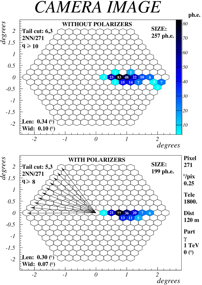
Figure 6: The upper plot shows the image produced in the standard camera by a MC 1 TeV $\gamma$-ray shower. The lower plot shows the image of the same shower in the polarizer camera described on the text. The arrows in the lower plot illustrate how the polarizers are arranged on the camera.

Fig. 6 shows the schematics of the setup which we shall use to take advantage of the radial polarization of the light in the image. A polarizer is laid on top of each of the camera photomultipliers (PMTs) with its transmitting axis pointing towards the center of the camera. The arrows in the lower figure indicate the direction of the polarizer axes. In the following we shall refer to the camera equipped with polarizers as polarizer camera as opposed to the standard camera without polarizers. The signal in the pixels of both cameras by a simulated $\gamma$-ray event is also displayed in the figure.

It is well known that the projection of the light density onto the ellipse major axis is correlated to the longitudinal development of the shower. Pixels closest to the camera center correspond to early stages in the shower development and those farthest away to its latest phases. The degree of radial polarization should thus increase slightly towards the center of the telescope where light comes mainly from higher up in the atmosphere.

Let us see how this setup may enhance a $\gamma$-ray signal in an IACT. Since night sky light is unpolarized, an immediate effect of this setup is to suppress 50% of the background light. In addition the images of off-axis showers are distributed randomly over the camera, which is to say that major axes do not point to the center of the camera. Since most of the hadron showers are off-axis, we expect the setup to reduce the hadronic background. Besides, the light in the tail and outer zones of the image will be substantially reduced and the image will be compacted. This is because the radial component of the polarization dominates close to the camera center. Fig. 7 illustrates this point for a simulated gamma and a simulated proton shower.

4 Monte Carlo Simulation

To study the proposed setup we have used a MC simulation based on the program CORSIKA 5.6 [9, D. Heck et al. 1998], slightly modified it to include the polarization of the Cherenkov light. We have selected the packages VENUS [23, K. Werner 1993] and GHEISHA [8, H. Fesefeldt 1985] to correspondingly simulate high and low energy hadronic interactions and EGS4  [18, W. R. Nelson et al. 1985] to simulate the electromagnetic interactions.

100 $\gamma$-initiated showers were generated at discrete primary energies in the range 200 GeV - 1.6 TeV in steps of 100 GeV and 100 proton-initiated showers at primary energies in the range 600 GeV - 4.8 TeV in steps of 300 GeV. The difference in the energy range of the simulated showers obeys to the fact that showers induced by $\gamma$-rays produce roughly three times more Cherenkov light that showers induced by protons. The telescope was always simulated as pointing to the zenith. Gamma showers were produced only in the zenith direction while protons were distributed isotropically within 3^∘ of the zenith. Observation level and magnetic field correspond to the HEGRA experiment site at El Roque de los Muchachos ($28^{\circ}$N, $17^{\circ}$E, 2200 meters a.s.l.) in the Canary Islands.

4.1 Detector Simulation

We shall simulate an IACT with the features of the telescope in the HEGRA system [6, A. Daum et al. 1997] but apply a number of simplifications. The reflector is represented by a single 8.5 m² parabolic mirror of 5 m focal length. The camera is located at the focal point and consists of 271 0.25^∘ diameter PMTs. We assume that a global $10\%$ photon conversion efficiency for the whole detector accounts for atmospheric attenuation, mirror reflectivity and QE of the PMTs.

In order to increase the statistics of our sample we image each individual EAS with $\sim 10^{4}$ telescopes homogeneously arranged inside a circle of 250 meters radius centered on the shower core. This procedure leads to a sample on the order of $10^{6}$ gamma events and $10^{6}$ proton events for each primary energy. Whilst the sampling fluctuations are faithfully represented, the sample suffers from a high shower to shower correlation.

We suppose that the polarizers are perfect, that is, they absorb no light polarized in the transmitting axis. The effect of a camera with and and without polarizers has been studied for each event. We also assume that the polarization vector suffers no change in the state of polarization upon reflection on the mirror. This should be a good approximation. We refer the reader to Ref. [21, J. Sanchez Almeida and V. Martinez Pillet 1992] for a complete discussion on the effects that a telescope has on polarized light.

The simulation also takes into account the effect of the night sky background (NSB) by assuming an intensity of $(1.7\pm 0.4)\cdot 10^{12}$ ph m^-2 sr^-1 s^-1. This number draws on experimental measurements at El Roque de los Muchachos [17, R. Mirzoyan and E. Lorenz] using a narrow angle detector in the 300-600 nm spectral range.

4.2 Trigger Condition

A critical factor in the IACT technique is the trigger threshold condition. The trigger threshold sets the limit to the accidental trigger rate mainly due to NSB. The polarizing filters reduce the NSB reaching the camera PMTs in a factor two, hence reducing the rate of accidental triggers. Conversely the trigger threshold must be different to accomplish the same rate of accidentals for a camera with and without polarizers. A trigger condition of two next neighbor pixels (NN) with at least 10 photoelectrons (phe) (as currently in use in the HEGRA system [13, A. Konopelko 1999]) was adopted for the simulation of the camera with no polarizers. The demand to obtain the same rate of accidental triggers leads to a trigger condition of two NN with at least 8 phe in the case of camera equipped with polarizers.

We shall concern ourselves with two different background conditions. To start with we shall deal with NSB corresponding to a dark night, i.e., with no moon present. Then we will consider a higher NSB condition as during twilight or in the presence of moonlight. In the latter case the NSB can grow up to a factor of 50  [14, D. Kranich et al. 1999] with respect to a moon-less night. In our simulation we have adopted an intermediate ten-fold factor increase.

In making moonlight observations different approaches have been followed, such as to insert filters in front of the PMTs [15] or to reduce the gain of the PMTs. We shall compare simplified versions of these techniques with the above-described arrangement of polarizers. Of course inserting filters and polarizers is a one step process and can not be strictly compared to changing PMT gain in an arbitrary value. Polarizers and filters may however be considered as a first step in reducing the NSB.

A different trigger condition was defined for each NSB condition and experimental setup. The trigger conditions are obtained by requiring the same probability of random triggers. They are tabulated in table 1.

In obtaining the effective area and energy threshold of the telescope, we have assumed a Crab-like $\gamma$-ray source of differential spectral index 2.6 and flux normalization factor $dJ_{\gamma}$ ($>$1 TeV) = 2.8 $\cdot$ 10^-11 s^-1 cm^-2 TeV^-1. Background protons have been simulated assuming a differential index 2.7 and flux normalization factor $dJ_{CR}$ ($>$1 TeV) = 1.6 $\cdot$ 10^-5 s^-1 cm^-2 sr^-1 TeV^-1. Only background events between $0^{\circ}$ and $3^{\circ}$ zenith angle have been considered.

4.3 Image Analysis

Cherenkov images are generally described in terms of the so-called Hillas image parameters  [10, A.M. Hillas 1985] (a second moment analysis of the intensity distribution of light in the camera). A two level so-called tail-cut is applied to extract the shower image from the light intensity on the pixels (as described e.g. in Ref. [20, M. Punch et al. 1992]). We have selected the values of the so-called picture and boundary tail-cuts to be above a certain threshold imposed by the fluctuations of the NSB. For the low NSB situation with no polarizers the image tail-cut matches the cut applied in the HEGRA experiment (6 phe for the picture tail-cut and 3 phe for the boundary tail-cut [13, A. Konopelko 1999]). When simulating the polarizer camera both cuts were tuned to obtain approximately the same probability of random occurrence and turned out to be 5 phe for the picture tail-cut and 3 phe for the boundary tail-cut.

Background-dominated pixels can be excluded by ways of this technique. Only then are image parameters computed. We have applied a set of super-cuts in agreement with those used by the HEGRA collaboration (see  [16, D. Petry et al. 1996]) and kept it constant over all the camera arrangements under discussion. This means that some room is still left open to optimize the cuts in the polarizer camera.

5 Results

The goal of this section is to estimate the performance of the proposed polarizer arrangement. We shall consider a detection and an analysis level.

In the detection level we shall compare the effective area of the telescope ($A_{eff}$) for $\gamma$- and hadron-initiated EAS. $A_{eff}$ is computed as:

$$A_{eff,\gamma}(E)=2\pi\int_{0}^{\infty}P_{\gamma}(E,r)\cdot rdr$$ (1)

where $P_{\gamma}(E,r)$ is the trigger efficiency or probability of detecting a gamma ray shower of primary energy $E$ at core distance $r$. For hadron-initiated EAS the integral the angle of incidence is also considered.

Each MC shower allows us to estimate the effective area as the total area covered by telescopes, multiplied by the fraction of the total number of simulated telescope positions for which the simulated telescope response gives raise to a trigger.

$$A_{eff,i}(E)=A_{tot}\times\frac{N_{tel,triggered}}{N_{tot}}$$ (2)

We calculate $A_{eff}$(E) as the average of $A_{eff,i}$(E) for all the simulated showers.

The differential $\gamma$ detection rate is obtained by weighing $A_{eff,\gamma}$ with the spectrum of the incident Very High Energy $\gamma$s. The threshold energy, $E_{th}$, is defined as the value of the energy for which the rate of detection of $\gamma$ showers is maximal. Although $E_{th}$ contains essentially the same information as $A_{eff}$, it has a more appealing physical meaning and it is easier to compare with experimental results and other simulations.

At the analysis level, a standard analysis based on the Hillas parameters [10, A. M. Hillas 1985] will be performed on both samples. On one hand the distributions of the most significant image parameters give some insight at the differences induced by the presence of the polarizers. On the other hand the quality factor obtained from the analysis will also be compared.

The two different scenarios of respectively low and high NSB described in section 4.2 will be separately analyzed and compared.

5.1 Low noise scenario

Fig. 8 shows the trigger probability for $\gamma$ and proton initiated events. For $\gamma$ events differences due to the introduction of the polarizers are more observable at low energies and close to the core, as expected from the total amount of light collected and the distribution of net polarization. For proton events the effect of the polarizers is more noticeable in the total number of triggered events than in the shape of the trigger distribution.

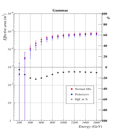
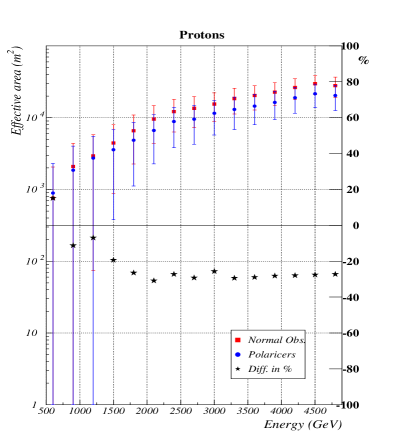
Figure 9: Shown here are the effective areas for $\gamma$ and proton showers for a standard and a polarizer camera. The right scale measures the percentage difference between the areas in both cameras.

Fig. 9 shows the effective area for $\gamma$ and proton initiated events. Two facts must be noted:

• $A_{eff}$(E) is always smaller when polarizers are used, both for $\gamma$ and protons.

• The loss in effective area is larger for protons than for $\gamma$s.

The conclusion can be drawn that although the background is reduced more strongly than the signal , this improvement does not compensate for the lost in statistics due to the reduction in triggers. The net reduction in the signal to noise ratio between the two cameras is of approximately 10%.

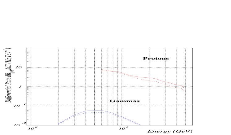
Figure 10: Differential rates as a function of energy for the standard camera (solid lines) and the polarizer camera (dashed lines).

Fig. 10 shows the differential rate as a function of primary energy for $\gamma$ and proton initiated events. The energy threshold at around 500 GeV compares reasonably well to the results in Ref. [13, A. Konopelko 1999] based in a detailed simulation of the HEGRA telescope system and matched to experimental data. Additionally, it is seen that the introduction of polarizers implies no significant difference in energy threshold but a small reduction of the effective area.

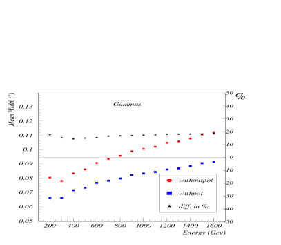
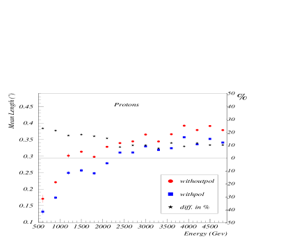
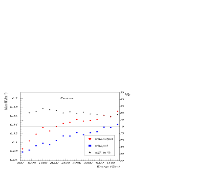
Figure 11: Comparison of the Hillas image parameters length (right) and width (left) in the standard and the polarizers camera, for $\gamma$s and protons. The absolute values are marked with circles and squares, while stars represent the percentage relative difference.

Plots in figure 11, described in more detail in the caption, compare the mean value of the image parameters length and width for $\gamma$ and proton initiated EAS as a function of energy for both cameras. The general trend is a reduction in both parameters. It reflects the fact that the photons in the tails of angular distributions show a lower radial polarization.

It has been found that the distribution of the Hillas $\alpha$ parameter is nearly unmodified. This is because in spite of the fact that shower images in the polarizer arrangement are narrower, the shower images also become shorter by approximately the same factor.

The effect of the polarizers on the quality factor for a standard set of super-cuts [16, D. Petry et al. 1996] has been also studied. Results indicate that the performance of the system is very similar with and without polarizers, depending on the energy range. However, given the approximations assumed in this work the result can not be considered a final answer. A detailed study for each given instrumental setup would be necessary.

5.2 High noise scenario

The previous section shows that the introduction of polarizers does not noticeably improve the performance of a telescope, although the signal to noise ratio increases. Notwithstanding this fact the arrangement could still be helpful when the amount of light arriving at the detector has to be reduced to be able to cope with an increased background level. Specific examples may be the need to adapt an instrument to be able to operate during twilight or in the presence of moon light.

Observations during twilight, or in the presence of the moon enable IACTs to extend their reduced duty cycle. The benefit lies not only in the increased event statistics and observation time, but also in the flexibility to efficiently cover the short term flux variations of VHE sources. Of course, there is a price to pay in the form of higher background.

Attempts to extend observation periods to high background conditions as observations with moonlight have consisted either in using special UV sensitive PMTs and blocking filters (since UV moonlight is blocked by the ozone layer) [19, Pare et al 1991],[4, Chantell et al 1995], [3, Bradbury et al 1996] [15, D. Pomarède et al. 2001] or reducing the PMT gain [14, D. Kranich et al. 1999]. Both approaches lead to an increase of the energy threshold of the telescope, the last alternative having yielded the best results to date.

Moonlight increases the amount of NSB by a factor of 3 to 5 during half moon up to a factor 30-50 during full moon [7, Dawson and Smith 1996] (when the telescope points 45^∘ away from the moon). In this section we will only consider situations where the background light is unpolarized, leaving for section 6 the discussion on polarized backgrounds.

To test the suitability of introducing polarizers during high background observations three different setups have been contemplated:

1. Reduced PMT gain in the standard camera.

2. Introduction of a grey filter on top of the standard camera, modeled by suppressing 50% of the collected photons.

3. Introduction of a polarizer camera.

Setup B , has been chosen to represent the easiest solution of just blocking a fixed percentage of the light arriving to the camera. Filters tried in IACTs are smarter [15, D. Pomarède et al. 2001] , selecting a range of wavelengths, but equally unrestricted in polarizations.

We have increased the NSB in our MC simulations in a factor 10. This factor is a realistic estimate of a real high background situation, such as a moonlight observation. The difference in noise among the three setups studied impose the need to tune first some parameters of the simulation. These are in particular $q_{0}$ (the trigger threshold for each pixel) and the two free parameters involved in the two level tail cut. The three of them have been adjusted to result on equal probabilities of accidental trigger, for the trigger, and random occurrence, for the two level cut, respectively. In practice, as we are dealing with integer numbers, probabilities are only approximately equal. It has to be kept in mind that setups B and C reduce NSB to the same level, leading to the same number of random triggers.

The results of our simulations can be summarized in two plots, showing the corresponding effective areas. Plot 12 represents the effectives areas as a function of energy when NSB is increased by a factor of 10 for case A and case C. The reductions in the total amount of events observed are larger than those shown previously due to the different thresholds, but the conclusions are very similar to those in the previous section: polarizers suppress more light in proton showers but differences do not seem important enough to justify its use.

Plot 13 compares the effect of polarizers and of simple light suppression. (labelled in the plots with 50%). From the left hand side plot it can be seen that the number of surviving gammas is higher for the polarizers case by a factor that goes from 50 to 100%. The right hand side plot shows that more protons survive, and the gain for protons is always smaller. Even an equal increase in protons and gammas would favor the use of polarizers, since the signal grows linearly with the number of events in the asymptotic Gaussian regime, while background grows only as the square root. The fact that the fraction is larger for gammas makes it more attractive.

6 Observations with polarized background light

While the considerations made in previous sections apply to unpolarized background light, attention must be paid to situations where the background has a definite polarization. The question of whether the use of polarizers could help in those situations can be partially answered from the results shown so far.

The most common case where polarized light constitutes an appreciable background is the one of linear polarization, normally caused by scattering. An important case is that of observation in moonlit nights, at a certain angular separation from the moon or at twilight, away from the sun. Light scattered at right angles to the moon or sun position acquires a high degree of polarization. See for example [1, I.K. Baldry and E. Bland-Hawthorn] and references therein. At least two simple arrangements of polarizers can be imagined as possible improvements for this situation. The first one is the polarizer camera discussed in the paper. The second one consists in a single polarizer whose transmitting axis is perpendicular to the dominant polarization of the background, to block a maximum amount of it.

Besides the reduction in background (which may be very important under some circumstances), the most important effect of both arrangements is the creation of ”non-uniformity” on the camera. The fraction of the polarizers aligned parallel to the direction of the background allows light to pass freely, increasing the background with respect to those perpendicular to it. A single polarizer oriented perpendicularly to the background polarization will suppress the light more efficiently depending on the position of the image on the camera (as discussed in section  2). Both effects should be taken into account in designing such a system.

7 Conclusions

We hope that this paper will help to clarify some of the properties of Cherenkov light polarization in EAS. We have pinpointed several aspects of the Cherenkov detection which may benefit from the consideration of the state of the light polarization. In particular we have considered $\gamma$/hadron separation, reduction of NSB and reduction of the trigger gate width, with its implications a further disminution of the NSB.

More specific results have been presented for the special case of IACTs. An experimental setup which uses the polarization to increase the significance of VHE gamma signals has been suggested. In this setup polarizing filters are arranged on top of each of the camera PMTs. The transmitting axes point to the camera center. We have studied the performance of this setup by means of a simplified MC simulation. Our conclusion is that the setup does not help in dark night observations but would be useful when the high NSB makes necessary to reduce the amount of light on the camera. In that case it amounts to an intelligent reduction of light.

Special attention must be paid to situations when the background light is polarized.

In this study some factors (such as the characteristics of the telescope, the composition of the hadronic background or the behavior of the polarizers) have been greatly simplified. At the same time the analysis has not been refined to fully exploit all of the advantages of the polarizer camera, as for instance by taking into account the shorter time profile of the Cherenkov photons or by redefining the set of super-cuts. A more detailed study featuring all the characteristics of a real detector and including experimental tests may prove rewarding.

Figure 4: Cherenkov light production height as a function of polarization angle for 10 MC gamma ray showers at 1 TeV and 10 MC hadron showers of 3 TeV at 3 degrees zenith angle. The first interaction point was fixed at 35 km above sea level. The vertical error bars represent the height interval where the mean value of $\theta_{pol}$ has been obtained. Since the distribution of $\theta_{pol}$ is asymmetric, a left and right width have been calculated representing the interval within 34 $\%$ of the events (equivalent to 0.5 $\sigma$ in a gaussian distribution) are contained at both sides of the median.

Figure 5: The upper plot shows the arrival mean time at different core distances for the set of MC events of the previous figure. The time origin of the y-axis is arbitrary. The lower plot displays the rms of the time distribution at different core distances. Set 1 corresponds to the polarization assumption and set 2 to the non-polarization assumption. Stars represent the difference between both sets, expressed in nanoseconds in the upper plot and as a percentage in the lower one. The plots are only meant to illustrate the general features of the arrival time distribution.

Figure 7: MC simulation of the polarization vector distribution on the IACT focal plane. On the left: 1 TeV gamma event of impact parameter close to the hump. Only one fourth of the camera is shown, the rest is empty. On the right: 3 TeV proton event at $3^{\circ}$ zenith angle and impact parameter close to the hump.

Figure 8: The upper plot represents the detection probability as a function of primary $\gamma$ energy for a standard (a) and a polarizer camera (b). The lower figure shows the same for proton events.

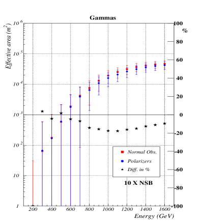
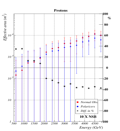
Figure 12: Effective areas as a function of energy for $\gamma$ and proton showers in setups A and C under ten times the NSB of a dark night. The right scale measures the percentage difference between the results obtained by both methods.

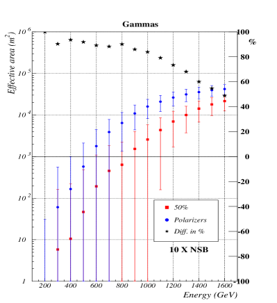
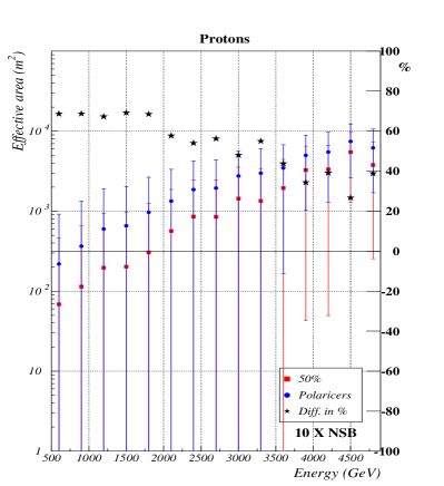
Figure 13: Effective areas for $\gamma$ and proton showers for two setups aiming at reducing the effect of NSB: light suppression using a filter (labelled 50%) and insertion of polarizers. The scale on the right axis measures the percentage difference between the results obtained in both setups.

	Low NSB (dark night)		High NSB
$FLUX_{NSB}$	$(1.7\pm 0.4)\cdot 10^{12}$		$(1.7\pm 0.4)\cdot 10^{13}$
ph m-2 sr-1 s-1	Without	With	Without	With	50%
$\geq$ 2NN/271	10 phe	8 phe	26 phe	19 phe	19 phe

Table 1: Trigger threshold conditions for the two NSB conditions and three experimental setups described in the text (camera with and without polarizers and 50% light suppression)

References

- [1] I.K. Baldry and J. Bland-Hawthorn 2000. MNRAS 000, 1-5 (2000).
- [2] B. Bartoli et al. 1998, ECRS (Alcalá) 405.
- [3] S.M. Bradbury et al. 1996, Towards a major Atmospheric Cherenkov Detector IV (Padova) 182
- [4] Chantell M., et al. (1995) ICRC (Rome) 2 544.
- [5] V. R. Chitnis and P. N. Bhat 1999, astr-ph/9902253 18 Feb 1999.
- [6] A. Daum et al. 1997, APh 8 1-11.
- [7] B. Dawson and A. Smith al. 1996. Technical report GAP-96-034, University of Adelaide.
- [8] H. Fesefeldt 1985, Aachen PITHA 85/02.
- [9] D. Heck et al. 1998, Report FZKA 6019 Forschungszentrum Karlsruhe.
- [10] A. M. Hillas 1985, Proc. ICRC (La Jolla) 3 445.
- [11] A. M. Hillas 1996, Space Science Reviews 75, 17-30.
- [12] J. V. Jelley 1958, Cherenkov Radiation and its Applications Ed. Pergamon Press.
- [13] A. Konopelko et al. 1999. Astrop. Phys. 10 275-289
- [14] D. Kranich et al. 1999 APh 12 65-74.
- [15] D. Pomarède et al. 2001. Aph 14 287-317.
- [16] D. Petry et al. 1996, A&A 311, L13.
- [17] R. Mirzoyan and E. Lorenz; Internal Report of the HEGRA collaboration.
- [18] W. R. Nelson et al. 1985, SLAC 265.
- [19] E. Pare et al. 1991, 22nd Int. Cosmic Ray Conf. (Dublin), 1, 492.
- [20] M. Punch et al. 1992, Nature, 358, 477.
- [21] J. Sanchez Almeida and V. Martinez Pillet 1992, A&A 260 543-555.
- [22] A. K. Tickoo 1999, ICRC (Salt Lake City) 4 255.
- [23] K. Werner 1993, Phys Rep 232 87.