Cas–A

X-ray spectral imaging and Doppler mapping of Cassiopeia A

We present a detailed X-ray spectral analysis of Cas A using a deep exposure from the EPIC-MOS cameras on-board XMM-Newton. Spectral fitting was performed on a 15$\times$15 grid of $20{\arcsec}\times 20{\arcsec}$ pixels using a two component non-equilibrium ionisation model (NEI) giving maps of ionisation age, temperature, interstellar column density, abundances for Ne, Mg, Si, S, Ca, Fe and Ni and Doppler velocities for the bright Si-K, S-K and Fe-K line complexes. The abundance maps of Si, S, Ar and Ca are strongly correlated. The correlation is particularly tight between Si and S. The measured abundance ratios are consistent with the nucleosynthesis yield from the collapse of a progenitor star of 12 $M_{\odot}$ at the time of explosion. The distributions of the abundance ratios Ne/Si, Mg/Si, Fe/Si and Ni/Si are very variable and distinctly different from S/Si, Ar/Si and Ca/Si. This is also expected from the current models of explosive nucleosynthesis. The ionisation age and temperature of both the hot and cool NEI components varies considerably over the remnant. Accurate determination of these parameters has enabled us to extract reliable Doppler velocities for the hot and cold components. The combination of radial positions in the plane of the sky and velocities along the line of sight have been used to measure the dynamics of the X-ray emitting plasma. The data are consistent with a linear radial velocity field for the plasma within the remnant with $v_{s}=2600$ km s^-1 at $r_{s}=153$ arc seconds implying a primary shock velocity of $4000\pm 500$ km s^-1 at this shock radius. The Si-K and S-K line emission from the cool plasma component is confined to a relatively narrow shell with radius 100-150 arc seconds. This component is almost certainly ejecta material which has been heated by a combination of the reverse shock and heating of ejecta clumps as they plough through the medium which has been pre-heated by the primary shock. The Fe-K line emission is expanding somewhat faster and spans a radius range 110-170 arc seconds. The bulk of the Fe emission is confined to two large clumps and it is likely that these too are the result of ablation from ejecta bullets rather swept up circumstellar medium.

1 Introduction

In this paper we present a detailed X-ray spectral analysis of the young supernova remnant Cassiopeia A with an angular resolution of the order 20 arc seconds over a field of view covering the full remnant. The data were obtained from an 86 kilosecond exposure of the XMM-Newton EPIC-MOS cameras to the source. The outstanding spectral grasp of XMM-Newton, i.e. the combination of sensitivity, X-ray bandwidth and spectral resolving power, coupled to this very long exposure time provides ample photon statistics for a full spectral modelling of each image pixel commensurate with the beam width of the XMM-Newton telescopes ($\sim$15 ″ Half Power Width), even for source regions of low surface brightness. This is illustrated in Fig. 1 which shows a broad band high resolution Chandra image of Cas A (Hughes et al. 2000) on which the pixel grid used in this analysis has been superimposed. Also drawn on this image is a contour indicating the region with good statistics and where the flux is not dominated by scattering. In addition, two samples of raw spectral data are shown, indicating the typical statistical quality in regions of high and low surface brightness.

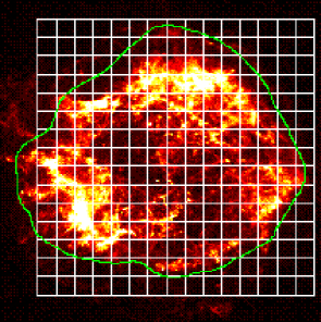
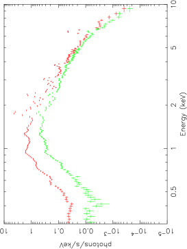
Figure 1: The pixel grid used in our analysis superimposed on the high angular resolution Chandra image of Cas A. The green contour indicates the region with good statistics and low scattering. Below are typical single pixel spectra from a high count and a low count region.

The energy resolution, gain stability and gain uniformity of the MOS-cameras allows significant detection of emission line energy shifts of order 1 eV or greater for prominent lines like Si-K, S-K and Fe-K. Proper modelling of these line blends with the aid of broad band spectral fitting, taking into account the non-equilibrium ionisation balance (NEI), allows an assessment, with unprecedented accuracy, of Doppler shifts and abundance variations of the X-ray emitting material across the face of the remnant with an angular resolution adequate enough to discriminate the fine knot structure seen by Chandra. The implications for the dynamical model of the remnant and for the origin and shock heating of the X-ray emitting ejecta will be highlighted as the key result of this investigation.

2 Spectral Fitting Analysis

We divided a 5′$\times$ 5 ′field of view of Cas A on a spatial grid containing 15$\times$15 pixels. This corresponds to a pixel size of $20{\arcsec}\times 20{\arcsec}$, slightly larger than the half-power beam width of XMM-Newton. Spectra were extracted using this grid and analysed on a pixel by pixel basis.

The spectral analysis was performed using the SRON SPEX (Kaastra et al. kaastra (1996)) package, which contains the MEKAL code (Mewe et al. mewe (1995)) for modeling thermal emission. We find that, even at the $20{\arcsec}\times 20{\arcsec}$ level, one thermal component does not model the data sufficiently well, particularly in describing both the Fe-L and Fe-K emission. We therefore choose as a minimum for representative modelling two NEI components for the thermal emission. In addition we incorporated the absorption measure as a free parameter and also introduced two separate redshift parameters, one for each plasma component.

The basic rationale behind a two component NEI model is that we expect low and high temperature plasma associated with a reverse shock and a blast wave respectively. While we obtain good fits using a two NEI model, we estimate that a contribution from a power law hard tail to the 4-6 keV continuum could be as high as 25$\%$. Since there is no evidence that the hard X-ray emission is synchrotron and it’s brightness distribution is very much in line with the thermal component (see Bleeker et al. bleeker (2001)), we feel that our fitting procedure is justified. In other words the combined high and low temperature NEI components will provide a good approximation to the physical conditions that give rise to the line emission.

The low temperature plasma component in our model implicitly assumes that the ejecta material, which largely consist of oxygen and its burning products (Chevalier & Kirshner chevalier (1997)), has been fully mixed regarding the contributing atomic species. In order to mimic a hydrogen deficient, oxygen rich medium we adopted a similar approach to that used by Vink et al. (1996), where they fixed the oxygen abundance of the cool component to a high value. We set the cool component abundances of O, Ne, Mg, Si, S, Ar and Ca to a factor 10000 higher than that of the hot component. It should be noted that 10000 is not a magic number, 1000 would suffice. The important point is that oxygen and the heavier elements are all dominant with respect to hydrogen so that oxygen rather than hydrogen is the prime source of free electrons in the plasma. The abundances of O, Ne, Mg, Si, S, Ar, Ca, Fe and Ni were allowed to vary over the remnant while the rest of the elemental abundances (He, C and N) were fixed at their solar values (Anders & Grevese anders (1989)).

Our model allows us to estimate the distribution over the remnant of the emission measure $n_{\rm e}n_{\rm H}V$, the electron temperature $T_{\rm e}$ and the ionisation age $n_{\rm e}t$ of the two NEI components as well as the distribution of the abundance of the elements (O, Ne, Mg, Si, S, Ar, Ca, Fe & Ni), the column density $N_{\rm H}$ of the absorbing foreground material, Doppler broadening of the lines and the redshift of the respective plasma components. Here $n_{\rm e}$ and $n_{\rm H}$ are the electron and hydrogen density respectively, $V$ is the volume occupied by the plasma and $t$ is the time since the medium has been shocked. The best fit model parameters were found and recorded for each pixel and it was thus possible to create maps of the various model parameters over the face of the remnant.

3 Doppler mapping

It is possible to accurately determine the Doppler shifts of Si-K, S-K and Fe-K since these lines are strong and well resolved. Doppler shifts of these lines have been calculated in two different ways.

After fits were made to the full spectrum we froze all the fit parameters. We selected the Si-K (1.72-1.96 keV), S-K (2.29-2.58 keV) and Fe-K (6.20-6.92 keV) bands for determining their respective Doppler velocities while ignoring all other line emission. We then do a fit to each line separately by starting from the full fit model parameters as a template and subsequently allowing only the redshift and the abundance of the relevant element to vary. This method provides a fine tuning of the redshift which in turn gives the Doppler velocity of the element under scrutiny.

Alternatively, using the same fit parameters we calculated the predicted continuum flux, $\rm Fp_{cont}$, and energy centroid of the lines, $\rm Ep_{line}$ and energy centroid of the continuum, $\rm Ep_{cont}$, for each line energy band in each pixel. Then using the raw events we calculated the measured total flux, $\rm F_{band}$ and energy centroid $\rm E_{band}$ in each band again for each pixel. The measured line flux was then estimated by subtracting the predicted continuum from the total flux in each band, $\rm F_{line}=F_{band}-Fp_{cont}$. The continuum centroid in a line energy band varies as a function of position over the remnant and the energy centroid for each band is the weighted sum of the line and continuum components. The measured line energy centroid was calculated by removing the contribution from the continuum.

$$E_{line}=(F_{band}\times E_{band}-Fp_{cont}\times Ep_{cont})/F_{line}$$

An estimate of the Doppler shift of the line is then given by $\Delta E=E_{line}-Ep_{line}$.

The Doppler shifts calculated by these two methods were in reasonable agreement indicating that the results were not sensitive to line broadening and lines close to the edges of the chosen energy bands.

line	$\rm Ep_{band}$	$\rm\Delta E_{N}$	$\rm\Delta E_{C}$	$\rm\Delta V$	$\rm\Delta E_{NEI}$	$\rm\Delta V_{NEI}$
	keV	eV	eV	km s-1	eV	km s-1
Si-K	1.847	0.55	0.53	94	3.89	630
S-K	2.439	0.31	0.53	99	2.52	310
Fe-K	6.566	2.95	1.60	143	24.2	1115

Table 1: Estimates of the mean errors associated with determining the Doppler velocities. $\rm\Delta V$ is the mean statistical error in the Doppler velocity estimated from the two dominant factors and $\rm\Delta V_{NEI}$ is the rms of the systematic correction provided by the NEI modelling.

The accuracy of the Doppler shift values depends on the ability of the NEI spectral model to predict the line blends combined with the uncertainties in the gain calibration of the detectors. Maps were constructed using the combined counts from the two cameras MOS 1 and MOS 2. The results were the same but with somewhat poorer statistics if only MOS 1 or MOS 2 were used. The readout directions of the central CCDs of MOS 1 and MOS 2 are set perpendicular to one another on the sky so we are sure that the line shifts are not due to systematic charge transfer losses as the events are read out. Thus there is convincing evidence that the observed line shifts are not due to instrumental gain variations or some other more subtle detector effect.

The statistical errors on the velocity estimates depend on the intrinsic energy resolution of the detectors, the number of counts detected in the line energy band and the error associated with estimating the continuum contribution in the line energy band. There are two dominant factors. Firstly the statistical error in determining the energy centroid $\Delta E_{N}\approx\sigma_{E}/\sqrt{(}N)$ where $\sigma_{E}$ is the rms width of the detector energy resolution at the line energy and $N$ is the total detected count. Secondly the statistical errors in the continuum bands which translate into errors in the temperature and flux determination for the continuum flux and hence yield a centroid error $\Delta E_{C}$.

Systematic errors on the Doppler velocities are introduced by improper modelling of the unresolved emission line blends within the Si-K, S-K and Fe-K line energy bands. The centroids of the line blends vary considerably over the remnant because of large differences in temperature and ionisation age. We have calculated the rms variation $\rm\Delta E_{NEI}$ of the band centroid $\rm Ep_{band}$ over the remnant. If the spectral modelling is correct then this systematic error should have been eliminated.

Estimates of the factors effecting the accuracy of the Doppler velocities over the remnant are given in Table 1. The velocity error $\rm\Delta V$ was calculated from the combination of the two statistical components. The velocity errors do vary over the face of the remnant since they depend on the surface brightness but for all the bright knots the errors in Table 1 are a good estimate.

4 Key results

Fig. 2 shows a typical spectral fit. All features of the measured spectrum are remarkably well represented by the modelling.

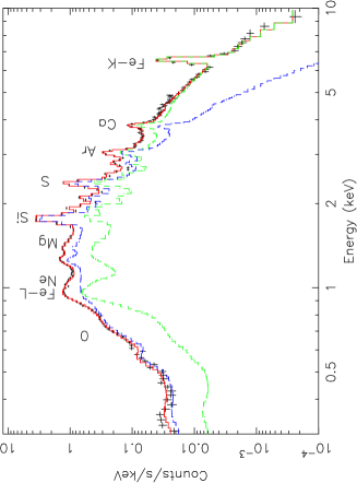
Figure 2: An example of a spectral fit within a single $20{\arcsec}\times 20{\arcsec}$ pixel - cool component in blue, hot component in green and full model in red.

Bivariate linear interpolation was used to transfer the model parameters, predicted fluxes etc. onto the grid of 1 arc second pixels. Fig. 3 displays maps of the ionisation age and temperature of the cool NEI component. This component is dominant in the line spectrum including Fe-L emission. The temperature distribution of the hot component is similar to (but not the same as) the cool component but with a temperature range 2-6 keV. The hot component is responsible for all the Fe-K emission and also dominates the continuum above 4 keV.

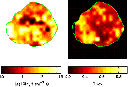
Figure 3: Spectral fit parameters for the cool component, ionisation age left-hand panel and temperature right-hand panel. The contour indicates the region with good statistics and low scattering.

Fig. 4 shows the ionisation age of the hot NEI component and the interstellar column density.

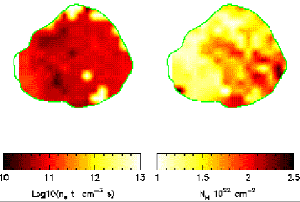
Figure 4: Ionisation age of the hot component and the interstellar column density. The contour indicates the region with good statistics and low scattering.

These plots demonstrate the amazing variability in the spectrum over the face of the remnant. The column density does exhibit some correlation with the surface brightness of the bright knots of the remnant presumably because of parameter coupling in the spectral fitting process. The $\rm N_{H}$ fitting is particularly sensitive to modelling of the O VIII emission 0.6-0.8 keV and Fe-L lines 1.0-1.5 keV. The mean column density is $1.5\times 10^{22}$ cm^-2 while the range is $1.0-2.5\times 10^{22}$ cm^-2. The variation of interstellar column density over the face of the remnant has previously been mapped by Keohane et al. (1996) using radio data. The distribution in their map is similar to Fig. 2 with high column density in the West due to a molecular cloud but the overall range of their column density derived from the equivalent widths of HI and OH is smaller, $1.05-1.26\times 10^{22}$ cm^-2.

Fig. 5 is a montage of abundance maps. Again we see considerable variations over the remnant. The Fe-L distribution comes from the cool component while the Fe-K and Ni are derived exclusively from the hot component.

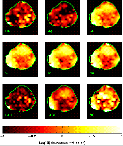
Figure 5: Abundance maps for the elements included in the spectral fitting. All are plotted on the logarithmic scale indicated by the bar at the bottom.

The distributions of Si, S, Ar and Ca, which are all oxygen burning products, are similar and distinct from carbon burning products, Ne and Mg, and Fe-L. Fig. 6 shows the variation in the ratios S/Si, Ar/Si and S/Si with respect to the abundance of Si. On the one hand these ratios clearly vary over the remnant but on the other hand, for a Si abundance range spanning more than two orders of magnitude, these ratios remain remarkably constant. The thick vertical bars indicate the mean and rms scatter of the ratio values.

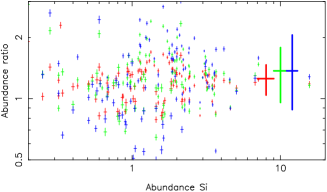
Figure 6: The variation in the abundance ratios of S/Si red, Ar/Si green and Ca/Si blue as a function of the Si abundance. The large error bars to the right indicate the mean and rms scatter for the three elements.

Line flux images were produced using an adaptive filter with a minimum beam count of 400 and maximum beam radius of 15 arc seconds. The raw event images from each line energy band were smoothed and then multiplied by the ratio of the predicted line flux to line plus continuum flux ratio in order to estimate the line flux. Fig. 7 shows the resulting line flux images colour coded with the Doppler velocity. The bottom left image is the colour coding used.

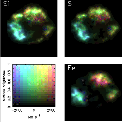
Figure 7: Doppler maps derived from Si-K, S-K and Fe-K emission lines. For each case the surface brightness of the line emission (after subtraction of the continuum) is shown colour coded with the Doppler velocity. The coding used is shown in the bottom left image.

The Doppler shifts seen in different areas of the remnant are very similar in the three lines. The knots in the South East are blue shifted and the knots in the North are red shifted. This is consistent with previous measurements, Markert et al. (1983), Holt et al. (1994), Vink et al. (1996). Moving from large radii towards the centre the shift generally gets larger as expected in projection. This is particularly pronounced in the North. At the outer edges the knots are stationary or slightly blue shifted. Moving South a region of red shift is reached indicating these inner knots are on the far side of the remnant moving away from us. The distributions of flux as a function of Doppler velocity are shown in Fig. 8. The distibutions for Si-K and S-K are very similar. The Fe-K clearly has a slightly broader distribution for the red shifted (+ve) velocities. The lower panel is the flux plotted in the Si velocity-S velocity plane showing the tight correlation between the Doppler shift measured for these lines. This plot was quite sensitive to small systematic changes in temperature, ionisation age or abundances in the spectral fitting since these can potentially have a profound effect on the derived Doppler velocities as indicated by the large values of $\rm\Delta V_{NEI}$ in Table 1.

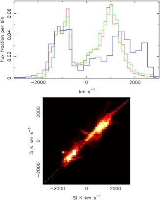
Figure 8: Flux distributions of Si-K (red), S-K (green) and Fe-K (blue) as a function of measured Doppler velocity. The lower panel shows the flux distribution in the Si velocity-S velocity plane.

The X-ray knots of Cas A form a ring because the emitting plasma is confined to an irregular shell. We searched for a best fit centre to this ring looking for the position that gave the most strongly peaked radial brightness distribution (minimum rms scatter of flux about the mean radius). The best centre for the combined Si-K, S-K and Fe-K line image was 13 arc second West and 11 arc seconds North of the image centre (the central Chandra point source). Using this centre the peak flux occured at a radius of 102 arc secs, the mean radius was 97 arc secs and the rms scatter about the mean radius was 24 arc seconds.

Given such a centre we can assign a radius to each pixel and using the Doppler velocity measured for each pixel we can map the flux into the radius-velocity plane. The result is shown in Fig. 9.

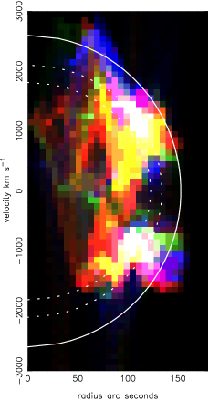
Figure 9: Flux distribution of Si-K (red), S-K (green) and Fe-K (blue) in the radius-velocity plane. The solid line is the best fit shock radius (see text). The outer dotted line indicates the peak of the Fe-K flux distribution and the inner dotted line indicates the mean radius of the Si-K and S-K emission.

5 Ionisation structure and abundance ratios

The models for nucleosynthesis yield from massive stars predict that the mass or abundance ratio $R_{\rm X/Si}$ of ejected mass of any element X with respect to silicon varies significantly as a function of the progenitor mass $M$. We show the observed mean values of $R_{\rm X/Si}$ as well as its rms variation in Table 2, together with the predictions for models with a progenitor mass of 11, 12 and 13 $\rm M_{\odot}$.

ratio	mean	rms	11 $\rm M_{\odot}$	12 $\rm M_{\odot}$	13 $\rm M_{\odot}$
O/Si	1.69	1.37	0.44	0.16	0.33
Ne/Si	0.24	0.37	0.59	0.12	0.33
Mg/Si	0.16	0.15	0.57	0.12	0.41
S/Si	1.25	0.24	0.87	1.53	0.88
Ar/Si	1.38	0.48	0.65	2.04	0.64
Ca/Si	1.46	0.68	0.63	1.62	6.56
FeL/Si	0.19	0.65	1.37	0.23	0.96
FeK/Si	0.60	0.51	1.37	0.23	0.96
Ni/Si	1.67	5.52	6.89	0.68	1.80

Table 2: Mean measured abundance ratios and rms scatter compared with theoretical predictions for progenitor masses of 11, 12 and 13 $\rm M_{\odot}$.

The observed abundance ratios for X equal to Ne, Mg, S, Ar, Ca and Fe-L (the iron of the cool component) are all consistent with a progenitor mass of 12.0$\pm$ 0.6 $\rm M_{\odot}$, where we used the grid of models by Woosley and Weaver (1995). In these models, most of the Si, S, Ar and Ca comes from the zones where explosive O-burning and incomplete explosive Si-burning occurs, and indeed as Fig. 6 shows these elements track each other remarkably well. Furthermore the average abundance ratio fits the expectation for a 12 $\rm M_{\odot}$ progenitor. The correlation between Si and S is remarkably sharp but not perfect, the scatter in Fig. 6 is real. These remaining residuals can be attributed to small inhomogeneities. Table 2 also indicates that the rms scatter of the abundances with respect to Si get larger as Z increases, S to Ar to Ca and indeed through to Fe and Ni. This is to be expected since elements close together in Z are produced in the same layers within the shock collapse structure while those of very different Z are produced in different layers and at different temperatures.

The Fe which arises from complete and incomplete Si burning should give rise to iron line emission. For both the Fe-L and Fe-K lines we see that iron abundance varies over the remnant but does not show any straightforward correlation with the other elements (there is a very large scatter in $R_{\rm Fe/Si}$). This is to be expected if most of the iron arises from complete Si burning. We return to the different morphologies of Si and Fe later in the discussion.

Ne and Mg are mostly produced in shells where Ne/C burning occurs, and the relative scatter in terms of $R_{\rm X/Si}$ is indeed much larger than for S, Ar and Ca (Table 2). Furthermore the abundance maps of Ne and Mg in Fig. 5 are similar and very different from the Si, S, Ar and Ca group.

The oxygen abundance is much higher than predicted by theory, contrary to all other elements. We cannot readily offer an explanation for this, but there are at least two complicating factors. As the XMM RGS maps show (Bleeker et al. 2001), oxygen has a completely different spatial distribution to the other elements (it is more concentrated to the North), and it is also much harder to measure due to the strong galactic absorption and relatively poor spectral resolution of the EPIC cameras at low energies.

The map of the ionisation age of the cool component shows a large spread. The average value at the Northern rim (few times $10^{11}$ cm^-3s) matches nicely the value derived from ASCA data (Vink et al. 1996). At the SE rim the ionisation age is much larger (cf. Vink et al. $4\times 10^{11}$ cm^-3s). We confirm this higher value, but also see that there is a large spread in ionisation age. It should also be noted that for ionisation ages larger than about $10^{12}$ cm^-3s the plasma is almost in ionisation equilibrium and therefore the spectra cannot be distinguished from equilibrium spectra; the extremely high values of $10^{13}$ cm^-3s in the easternmost part of the remnant (Fig. 3) are therefore better interpreted as being just larger than $10^{12}$ cm^-3s. There is also a region of very low ionisation age (less than $3\times 10^{10}$ cm^-3s) stretching from East to West just above the centre of the remant. This region also has a very low emissivity (i.e. low electron density) and can be understood as a low density wake just behind and inside of the shocked ejecta.

The hot component has a more homogeneous distribution of ionisation age, centered around $10^{11}$ cm^-3s, again consistent with the typical value found by Vink et al. (1996) but in that case integrated over much larger areas. We have now clearly resolved this component spatially.

6 Dynamics

In the radius-velocity plane the flux from a thin shell of radius $\rm r_{s}$ expanding at velocity $\rm v_{s}$ is expected to form an ellipse which intersects the radius axis at $\rm r_{s}$ and the velocity axis at $\rm\pm v_{s}$. We expect the velocity to increase with radius and for simplicity we can assume that the velocity field within the spherical volume is given by a linear form

$$\rm v(r)=\frac{v_{s}}{(r_{s}-r_{o})}(r-r_{o})$$

where $\rm v_{s}$ is the postshock velocity of material at the shock radius $\rm r_{s}$ and $r_{o}$ is the radius within the remnant at which the velocity falls to zero. From the analysis of the Chandra data, (Gotthelf et al. 2001), we have an estimate of $\rm r_{s}=153$ arc seconds. Adopting such a spherically symmetric velocity field precludes the possibility that the expansion is wildly asymmetric. In the plane of the sky the outer shock seen both in radio and X-ray images is remarkably circular (see for example the Chandra X-ray image scaled to highlight the faint outer filaments, Gotthelf et al. 2001). We therefore think it is unlikely that the velocity field or shock radius is very different along the line of sight. Assuming values for $\rm v_{s}$ and $\rm r_{o}$ we can calculate the radius of each pixel within the spherical volume from the observed radius on the plane of the sky and the Doppler velocity (along the line of sight). As the parameters are changed so the fractional rms scatter, $\rm\Delta r/r$, of the flux about the mean radius varies. The top left panel of Fig. 10 shows the variation in $\rm\Delta r/r$ as a function of $\rm r_{o}$ and $\rm v_{s}$.

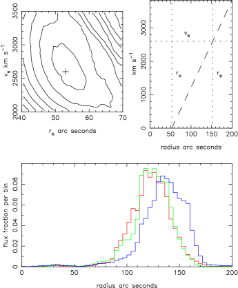
Figure 10: The velocity field which gives the minimum normalised shell thickness $\rm\Delta r/r$. Each contour interval in the top left plot corresponds to a $\sim 2$% increase in shell thickness. The lower panel shows the deprojected flux distribution of Si-K (red), S-K (green) and Fe-K (blue) as a function of radius from the centre of the remnant.

The minimum scatter of 0.16 is found at $\rm r_{o}=53$ arc seconds and $\rm v_{s}=2600$ km s^-1. The velocity field which gives the minimum shell thickness is shown in the top right-hand panel. This result is very similar to the velocity field of an isothermal blast wave, Solinger et al. (1975), but we would like to stress this does not imply that Cas A has entered this phase of it’s evolution. The remnant is almost certainly in between the ejecta-dominated and the Sedov-Taylor stages as modelled in detail by Truelove and McKee (1999). The lower panel of Fig. 10 shows the deprojected flux distributions as a function of radius in the spherical volume. The Si-K and S-K distribution match quite closely. The Fe-K distribution is somewhat broader and peaks at a larger radius. The deprojected Si-K and S-K flux distributions are very similar to the emissivity profiles derived from the Chandra data (Gotthelf et al. 2001) although their analysis was for a section of the remnant while the profiles in Fig. 10 are the average over the full azimuthal range. The solid semi-circular line in Fig. 9 is the best fit with $\rm r_{s}=153$ arc seconds and $\rm v_{s}=2600$ km s^-1. The inner dotted line shows the mean radius of the combined Si-K and S-K flux and the outer dotted line shows the peak of the Fe-K distribution. The outer reaches of the Fe-K distribution straddle the shock radius derived from the Chandra image.

The MOS energy resolution cannot separate the red and blue components when they overlap. If we see both the distant red shifted shell and nearer blue shifted shell in the same beam the line profile is slightly broadened but the centroid shift is diminished. The observed Doppler velocities and the best fit value for $\rm v_{s}$ may be slightly biased by this ambiguity, however most beams appear to be dominated by either red or blue shifted knots and therefore this bias is expected to be small. It is fortuitous that the X-ray emission is distributed in clumps rather than a thin uniform shell since this enables us to measure the Doppler shift with a modest angular resolution without red and blue components in the same beam cancelling each other out.

The left-hand panel of Fig. 11 is a composite image of the remnant seen in the Si-K, S-K and Fe-K emission lines. The solid circle indicates the $\rm r_{s}=153$ arc seconds and the dashed circle is the mean radius of the Si-K and S-K flux $\rm r_{m}=121$ arc seconds. The X-ray image of the remnant provides coordinates x-y in the plane of the sky. Using the derived radial velocity field within the remnant we can use the measured Doppler velocities $\rm v_{z}$ to give us an estimate of the z coordinate position of the emitting material along the line of sight thus giving us an x-y-z coordinate for the emission line flux in each pixel. Using these coordinates we can reproject the flux into any plane we choose. The right-hand panel of Fig. 11 shows such a projection in a plane containing the line-of-sight, North upwards, observer to the right.

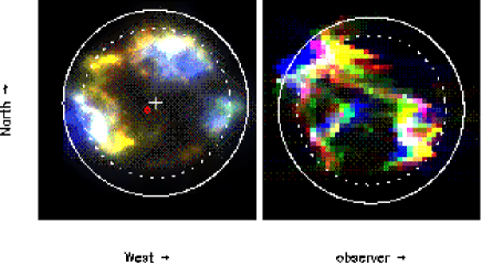
Figure 11: The left-hand panel is an image of Si-K (red), S-K (green) and Fe-K (blue). The small red circle indicates the position of the Chandra point source. The white cross is the best fit centre from the fitting of the radial distribution. The right-hand panel is a reprojection of the same line fluxes onto a plane containing the line of sight, North up, observer to right. In both panels the outer solid circle is the shock radius $\rm r_{s}=153$ arc seconds and the inner circle is the mean radius of the Si-K and S-K flux.

In this reprojection the line emission from Si-K, S-K and Fe-K are reasonably well aligned for the main ring of knots. The reprojection is not perfect because the MOS cameras are unable to resolve components which overlap along the line-of-sight and this produces some ghosting just North of the centre of the remnant. In the plane of the sky Fe-K emission (blue) is clearly visible to the East between the mean radius of the Si+S flux and the shock radius. Similarly in the reprojection Fe-K emission is seen outside the main ring in the North away from the observer. The Si+S knot in the South away from the observer in the reprojection is formed from low surface brighness emission in the South West quadrant of the sky image. The X-ray emitting material is very clumpy within the spherical volume and is indeed surprisingly well characterised by the doughnut shape suggested by Markert et al. (1983). However the distribution is distinctly different to that obtained in similar 3-D studies of the optical knots, Lawrence et al. (1995).

The expansion of Cas A has been measured in various ways; using the proper motion of optical knots (van den Bergh and Kamper 1983, Fesen et al. 1987, Fesen et al. 1988), from the proper motion of radio knots (Anderson and Rudnick 1995), using Doppler shifts of spectral lines from optical knots (Reed et al. 1995, Lawrence et al. 1995), Doppler shift of X-ray line complexes (Markert et al. 1983, Holt et al. 1994 and Vink et al. 1996) and the proper motion of X-ray knots (Vink et al. 1999). These methods identify a number of distinct features with different dynamics; Quasi Stationary Flocculi (optical QSF), Slow Radio Knots in the South West (SRK), the main ring of radio knots, the main ring of X-ray knots (continuum + lines 1-2 keV), Fast Moving Knots (optical FMK) and Fast Moving Flocculi (optical FMF).

In proper motion studies it is conventional to express the motion as an effective expansion time $\rm t_{ex}=R/V$ (years) where $R$ is the radius of the feature/knot from some chosen centre (arc seconds) and $V$ is the proper motion (arc secs/year). The deceleration parameter, the ratio of the true age over the expansion age, can be estimated as $\rm m=t_{age}/t_{ex}$. There is no need to deproject the radius or velocity to estimate $m$. However if we then wish to estimate a true expansion velocity the R must be deprojected but still the ratio $R/V$ will remain constant. Doppler measurements allow some form of deprojection and measured radii on the sky can be converted to actual radii within the volume of the remnant as described in the previous section. Given a radius in arc seconds $r_{as}$ and velocity in km s^-1 $\rm v_{kms}$ we can calculate an expansion time in years $\rm t_{ex}$ assuming a distance in kpc $\rm d_{kpc}$, $\rm t_{ex}=4.63\times 10^{3}r_{as}d_{kpc}/v_{kms}$. Previous authors have used combinations of these measurements to refine estimates of the age and/or distance. Alternatively we can adopt some age and distance and compare the radii and expansion velocities of the various components. The original explosion probably occured in 1680 (Ashworth 1980) so the age in 2000 is $\rm t_{age}=320$ years. Distance estimates have varied over the years but recent studies (Reed et al. 1995) have settled on $3.4^{+0.3}_{-0.1}$ kpc.

Table 3 gives estimates of the expansion parameters for the different components. Those marked with an asterisk are from proper motion studies which estimate the expansion time or the deceleration parameter directly. For these the $\rm r_{as}$ value has been estimated and the $\rm v_{s}$ calculated using the measured expansion time. From the Doppler measurements we get a measurement of $\rm r_{s}$ and $\rm v_{s}$ which are then used to estimate the expansion time or the deceleration parameter. Proper motion studies of X-ray emission track the movement of shock features in the plane of the sky while X-ray emission line Doppler measurements estimate the velocity of the postshock plasma $\rm v_{s}$ along the line of sight. The shock velocity $\rm u_{s}$ is related to the postshock plasma velocity, $\rm v_{s}=\alpha u_{s}$. The factor $\rm\alpha$ depends on the thermodynamics of the shocked gas but ranges between 0.58 for isothermal to 0.75 for adiabatic conditions, see for example Solinger et al. (1975). The present X-ray emission line (Xline) results in Table 3 have been calculated from the derived velocity field parameters, $\rm r_{s}=153$ and $\rm v_{s}=2600$ using a mean value of $\rm\alpha=0.65$. The error quoted reflects the uncertainty in this factor. The FMF are at large radii so it is likely that the deprojection correction is small and the value of 168 arc secs quoted is in fact the mean radius in the plane of the sky. For the SRK in the South West sector and the QSF the values quoted for $\rm r_{s}$ are just reasonable guesses.

	$\rm v_{kms}$	$\rm r_{as}$	$\rm t_{ex}$	m
QSF*	$370\pm 300$	$\sim 105$	$4470\pm 2300$	$0.07\pm 0.06$
SRK*	$656\pm 16$	$\sim 100$	$2100\pm 360$	$0.15\pm 0.02$
Radio*	$2848\pm 100$	$\sim 110$	$604\pm 12$	$0.51\pm 0.02$
Xline	$4000\pm 500$	$153\pm 5$	$537\pm 70$	$0.60\pm 0.07$
1 keV*	$3456\pm 105$	$\sim 110$	$501\pm 15$	$0.63\pm 0.02$
FMK	$5290\pm 90$	$105\pm 1$	$312\pm 9$	$0.98\pm 0.03$
FMF*	$8816\pm 28$	$168\pm 6$	$300\pm 9$	$0.99\pm 0.03$

Table 3: The expansion parameters for radio, optical and X-ray emissions. * indicates proper motion studies. The results from this paper are given in the line labelled Xline (see text for details).

The expansion time and deceleration parameters derived from the observed Doppler shifts of the Si-K, S-K and Fe-K lines (Xline in Table 3) are in reasonable agreement with the radio proper motion observations (Anderson and Rudnick, 1995) and in good agreement with the soft X-ray proper motion measurements of Vink et al. (1999) (1 keV in Table 3).

7 Discussion

The tight correlation between the variation in abundance of Si, S, Ar, Ca over an absolute abundance range of two orders of magnitude is strong evidence for the nucleosynthesis of these ejecta elements by explosive O-burning and incomplete explosive Si-burning due to the shock heating of these layers in the core collapse supernova. Full mixing of the burning products is implied by the excellent fit to the plasma model. However the Fe emission, both in the Fe-K and the Fe-L lines, does not show this correlation in any sense. A significant fraction of the Fe-K emission is seen at larger radii than Si-K and S-K as convincingly demonstrated in our Doppler derived 3-D reprojection, Fig. 11. Moreover the Fe-K emission is patchy, reminiscent of large clumps of ejecta material, rather than shock heated swept up circumstellar material. In fact the bulk of the Fe-K emission arises in two limited regions possibly indicating that the core collapse threw off material in two opposing clumps which we clearly see in Fig. 11. If we interprete these Fe-rich ejecta as the nucleosynthesis product of complete explosive burning of the Si-layer, spatial inversion of the O- and Si-burning products has occurred and large scale bulk mixing of the explosion products is an inevitable consequence. A similar conclusion was obtained by Hughes et al. (2000) for ejecta material at the east side of the remnant based on the morphological features of the high spatial resolution Chandra data.

The Fe-K emission requires a relatively high temperature in the range 2-6 keV. This temperature cannot be generated by the reverse shock wave, but only by the primary blast wave. Heating is certainly provided by the primary shock but preheating of the ambient medium by clumps that move ahead of the primary shock could contribute, see Hamilton (1985).

In the plane of the sky image Fig. 11 the Fe-K emission to the East is at a radius of 140 arc seconds, near the primary shock, with an implied shock velocity of $\rm u_{s}$ in the range 3500-4500 km s^-1 (see previous section). It is coincident with a cluster of three FMFs, 4,5,6 listed by Fesen et al. (1988). They all have a proper motion of $0.52\pm 0.05$ arc secs yr^-1 and a mean radius from the expansion centre in 1976 of $149\pm 3$ arc seconds. Assuming a distance of 3.4 kpc and age in 1976 of 296 years this corresponds to a transverse velocity of $8170\pm 790$ km s^-1 and a deceleration parameter of $m=1.0\pm 0.1$. The same Fe-K emission is also coincident with the radio knots 89,90,92 and 93 listed by Anderson and Rudnick (1995). These have a mean proper motion of $0.26\pm 0.01$ arc secs yr^-1 and a mean radius from the expansion centre in 1987 of $136\pm 3$ arc seconds. This corresponds to a transverse velocity of $4117\pm 160$ km s^-1 and a deceleration parameter of $m=0.59\pm 0.02$. These radio knots also correspond to the bow shock feature D identified using morphology and polarimetry by Braun, Gull & Perley (1987). They estimate the Mach number of this feature as 5.5, the highest in their list of 11 such features.

The Fe-K emission at large radii is highly reminiscent of SNR shrapnel discovered by Aschenbach et al. (1995) around the Vela SNR. These are almost certainly bullets of material which were ejected from the progenitor during the collapse and subsequent explosion. They would initially be expected to have a radial velocity less than the blast wave but as the remnant develops, and the shock wave is slowed by interaction with the surrounding medium, the bullets would overtake the blast wave and appear outside the visible shock front as is the case in Vela. It was suggested by Aschenbach et al. (1995) that the X-ray emission from the Vela bullets arises from shock-heating of the ambient medium by supersonic motion. If this is the case the X-rays will be seen from Mach cones which trail the bullets extending back towards the centre of the remnant.

The generation of radio emission associated with the deceleration of ejecta bullets has been discussed at length by several authors, Bell (1977), Braun, Gull & Perley (1987), Anderson and Rudnick (1995). The optical emission arises from shocks penetrating dense ejecta clumps. When these internal shocks have crossed the clump deceleration sets in accompanied by a strong turn-on of radio synchrotron emission. Electrons are accelerated in the bow-shock and the magnetic field is amplified in shearing layers between the dense ejecta and the external medium. The amplified magnetic field in the wake of ejecta bullets is predominately radial in agreement with radio polarization measurements, Anderson, Keohane and Rundick (1995). The supersonic flow associated with this scenario has been simulated by Coleman & Bicknell (1985). The same situation could also give rise to X-ray emission. The bulk of the electrons are heated to $\sim 3$ keV by the bow shock. As the shocked material drifts back into the wake the plasma slowly comes into ionization equilibrium and X-ray line emission is produced. Our analysis of the abundances clearly indicates that the matter responsible for the line emission is ejecta and this must have been ablated from the bullets rather than swept up by the shock. The velocities of both the radio and X-ray emission in the East are about half that of the optical. This is consistent with the peak of the radio and X-ray emission falling in the wake of the bullet trailing behind the peak of the optical emission.

What is the heating mechanism responsible for the cool component? Our present analysis clearly indicates this component is dominated by ejecta material. It is conventional to assume that the primary source of ejecta heating which produces the bright ring of X-ray emission in Cas A is the reverse shock (McKee 1974, Gull 1975). However the primary shock seen in X-rays and radio at a radius of 150 arc seconds is not very bright and it is not clear that the reverse shock has been or is presently very strong. The Chandra image shows much fragmentation consistent with dense bullets and it is likely that significant heating arises, again, from the interaction of these bullets with the material pre-heated by the primary shock.

- (1) Anders, E., Grevese, N., 1989, Geochimica et Cosmochimica Acta, 53, 197
- (2) Anderson, M.C., Rudnick, L. 1995, ApJ. 441, 307
- (3) Anderson, M.C., Keohane J.W., Rudnick, L. 1995, ApJ. 441, 300
- (4) Aschenbach B., Egger, R. & Trümper, J. 1995, Nature 373, 587
- (5) Ashworth, W.B. 1980, J. Hist. Astr., 11, 1
- (6) Bell, A.R. 1977, Mon.Not.R.astr.Soc 179, 573
- (7) Bleeker, J.A.M., Willingale, R., van der Heyden, K.J., et al., 2001, A&A, 365, L225,
- (8) Braun, R., Gull, S.F., & Perley, R.A. 1987, Nature, 327, 395
- (9) Chevalier, E., Kirshner, R.P., 1979, ApJ, 233, 154
- (10) Coleman, C.S., & Bicknell, G.V. 1985, Mon.Not.R.astr.Soc 214, 337
- (11) Fesen, R.A., Becker, R.H., Blair, W.P. 1987, ApJ 313, 378
- (12) Fesen, R.A., Becker, R.H. & Goodrich, R.W. 1988, Ap.J. 329, L89
- (13) Gotthelf, E.V., Koralesky, B., Rudnick, L., Jones, T.W., Hwang, U. and Petre, R. 2001, Ap.J. 552, L39
- (14) Gull S.F. 1975, Mon.Not.R.astr.Soc 171, 263
- (15) Hamilton, A.J.S. 1985, Ap.J., 291, 523
- (16) Holt, S.S., Gotthelf, E.V., Tsunemi, H., Negoro, H. 1994, PASJ 46, L15
- (17) Hughes, J.P., Rakowski, C.E., Burrows, D.N. and Slane, P.O. 2000, Ap.J. 528, L109
- (18) Kaastra, J.S., Mewe, R., Nieuwenhuijzen, H.1996, in UV and X-ray Spectroscopy of Astrophysical and Laboratory Plasmas, p. 411, eds. K. Yamashita and T. Watanabe, Tokyo, Univ. Ac. Press
- (19) Keohane, J.W., Rudnick, L., & Anderson, M.C., 1996, Ap.J. 466, 309
- (20) Lawrence, S.S., MacAlpine, G.M., et al. 1995, A.J. 109, 2635
- (21) Markert, T.H., Canizares, C.R., Clark, G.W., Winkler, P.F. 1983, apJ 268, 13
- (22) McKee C.F. 1974, Ap.J. 188, 335
- (23) Mewe, R., Kaastra, J.S., Liedahl, D.A., 1995, Legacy 6, 16
- (24) Reed, J.E., Hester, J.J., Fabian, A.C., Winkler, P.F. 1995, ApJ 440, 706
- (25) Solinger, A., Rappaport, S. and Buff, J. 1975, Ap.J. 201, 386
- (26) Truelove, J.K. & McKee, C.F. 1999, Ap.J.Supp.Ser. 120, 299
- (27) van den Bergh, S., Kamper, K.W. 1983, ApJ 268, 129
- (28) Vink, J., Kaastra, J.S., & Bleeker, J.A.M., 1996, A&A, 307, L41
- (29) Vink J. et al, 1999, A&A 344, 289
- (30) Woosley, S.E. & Weaver, T.A. 1995, Ap.J.Supp.Series, 101, 181