Confidence limits of evolutionary synthesis models

Evolutionary synthesis models are a fundamental tool to interpret the properties of observed stellar systems. In order to achieve a meaningful comparison between models and real data, it is necessary to calibrate the models themselves, i.e. to evaluate the dispersion due to the discreteness of star formation as well as the possible model errors. In this paper we show that linear interpolations in the $\log M-\log t_{k}$ plane, that are customary in the evaluation of isochrones in evolutionary synthesis codes, produce unphysical results. We also show that some of the methods used in the calculation of time-integrated quantities (kinetic energy, and total ejected masses of different elements) may produce unrealistic results. We propose alternative solutions to solve both problems. Moreover, we have quantified the expected dispersion of these quantities due to stochastic effects in stellar populations. As a particular result, we show that the dispersion in the ${}^{14}\mathrm{N}/^{12}\mathrm{C}$ ratio increases with time.

1 Introduction

Since their early introduction (Tinsley 1980), evolutionary synthesis models have evolved to increase our understanding of the evolution of stellar populations in the Universe. The improvement of the observational capabilities has forced the model developers to include more realistic physical ingredients in the models (atmosphere models, grids of tracks covering all the evolutionary phases, etc…) to interpret the new data. Thus, evolutionary synthesis models have become a useful tool to understand the properties of observed stellar systems and to test the validity of different evolutionary tracks. The improvements of synthesis models for star-forming regions comprise mainly the inclusion of new physical inputs and the extension of the output results to more observables.

Nevertheless, several aspects of synthesis models are still largely perfectible. An analysis of the way in which homology relations of massive stars (implicitly used in evolutionary tracks interpolations and isochrone computations) should be modified according to the assumed mass-loss rate, and the inclusion of such new relations into the models, still need to be performed. Additionally, the mathematical approximations used to estimate the lifetimes of massive stars must be carried out carefully, otherwise they could produce unphysical results. Finally, the dispersion in the model output parameters due to the discreteness of stellar populations has been evaluated only in a few cases.

This work is the third paper of an on-going series whose the objective to study the oversimplifications and the possible biases of the evolutionary synthesis models for starburst regions, and to assess the confidence limits of their outputs. The global structure of the project is the following: Paper i (Cerviño et al. 2000b) has been devoted to the study of the confidence limits of synthesis models due to the discreteness of real stellar populations. In Paper ii (Cerviño et al. 2001b) we have investigated the Poissonian dispersion due to finite populations in non-time-integrated observables, its quantitative evaluation and implementation on codes with an analytical approximation of the Initial Mass Function (IMF), as well as its relation with the dispersion in the output results of Monte Carlo simulations. In this paper we present an analytical approximation to the Supernova rate (SNr) calculations in starburst galaxies and the problems related with its determination in evolutionary synthesis codes. We also study the influence of the interpolations in time-integrated quantities (kinetic energy, $E_{kin}$, and total ejected masses of different elements, $y_{z}$) and propose a more precise interpolation technique in order to avoid the unphysical results obtained by the previous models. Some improvements of the interpolation techniques of evolutionary tracks used in synthesis models will be presented in Paper iv (Cerviño 2001 in preparation). We will complete the series with a global study of the expected dispersion as a function of different star-formation laws (continuous and extended star formation).

In section 2 we present the evolutionary synthesis code used. In Section 3 we present an analytical estimate of the SNr and how it is computed in evolutionary synthesis models. In Section 4 we show how the released kinetic energy and the ejected masses are computed, and we estimate their Poissonian dispersions and bias due to different computation techniques. Finally we draw our conclusions in Section 5. All the results of this paper are available in tabular form in our web server at http://www.laeff.esa.es/users/mcs/.

2 The evolutionary synthesis model

Since evolutionary synthesis calculations rely on the properties of stars with far more mass values than available from stellar evolution calculations, one possible source of error is the method used to interpolate between the available stellar tracks.

A few works deal with this problem analytically, either proposing analytical formulations for some phases of the stellar evolution (Tout et al. 1996), or using an analytical population synthesis code (Plüschke et al. 2001). One advantage of analytical formulations is that the functional dependence of the output quantities may be obtained.

In order to understand and quantify the errors introduced by synthesis codes for star forming regions, we summarize the main characteristics of synthesis models with non-analytical formulations and the methods used to compute several parameters.

1. Most synthesis models interpolate in tables of evolutionary tracks. Such tables are discrete in their mass and time entries. When one wants to obtain the luminosity $L$, the effective temperature $T_{\mathrm{eff}}$, or other properties, including quantities which change abruptly along the evolutionary sequence (e.g. surface abundances), homology relations are assumed to describe with sufficient accuracy the dependence of these quantities with the initial stellar mass. Therefore, interpolations in the $\log M-\log A_{k}$ plane, where $M$ is the initial mass and $A_{k}$ is a generic stellar property at a given evolutionary stage, are usually performed. Additional interpolations in the $\log M-\log t_{k}$ plane are performed to obtain isochrones, and their validity will be examined in this paper. Whatever the approach is (fully analytical or table interpolation), continuity of the stellar properties is assumed. The problem of discontinuities in evolutionary tracks will be discussed in Paper iv.

2. To calculate the integrated properties of the stellar population (e.g., the luminosity in a given band) a numerical integration over the IMF-weighted isochrones is always needed. Two main approaches are used: either the IMF is binned into a grid of $N$ initial masses, $M_{i}$, and then, all stars belonging to the same mass bin are assumed to have exactly the same properties, or the IMF is sampled with Monte Carlo simulations, and then each individual star is evolved and the isochrone integration is performed adding the evolved stars.

   To avoid a bias due to the choice of the mass bin, a dynamical mass grid can be used within the first method (Meynet 1995, Schaerer and Vacca 1998, or Starburst99 Leitherer et al. 1999): at each computed age, the differences in $L$ and $T_{\mathrm{eff}}$ between two stars of initial masses $M_{i}$ and $M_{i+1}$, respectively, are constrained to be lower than a given resolution $\Delta L$ and $\Delta T_{\mathrm{eff}}$. Note that the resulting mass grid will be different at different ages: the total number of bins $N$ and the $M_{i}$ values vary from one computed age to another (i.e., it is a dynamical mass grid). Such method assures that the H–R diagram is mapped in a continuous way and all the relevant evolutionary phases for the given age (i.e. the isochrones) are included in the computations.

   In the case of Monte Carlo simulations, either a high number of simulations or a high number of stars in each individual simulation are needed to produce a well mapped isochrone. As a first order estimation, one simulation with 10⁵ stars in the mass range 2 – 120 M_⊙ is required (as used in Mas-Hesse and Kunth 1991) to obtain Ultraviolet and optical luminosities similar to those of analytical-IMF models. However, the dispersion of Monte Carlo simulations depends on the considered observable. Monte Carlo simulations have the advantage of allowing the straightforward computation of the standard deviations and the confidence levels due to the discreteness of the stellar population, provided the number of simulations performed is high enough. An additional advantage is that Monte Carlo simulations take into account fast evolutionary phases that may be lost in analytical simulations. The required number of simulations needed to obtain a satisfactory estimate of the dispersion can be estimated comparing the mean values of the outputs with the results of analytical codes as far as they must to coincide (at least for observables not related with fast evolutionary phases).

   In both cases, caution must be taken if the evolutionary tracks present discontinuities (this subject is addressed in Paper iv).

3. The final element of synthesis codes is the age resolution (or time step) used to compute the integrated properties of simple stellar populations, i.e. instantaneous bursts. A sufficient temporal resolution, depending a priori on the observable, is needed to assure accurate convolutions over other arbitrary star-formation histories (e.g., the case of constant star formation, subject addressed in Paper v).

For this study we have used the updated version of the evolutionary synthesis code presented in Mas-Hesse and Kunth (1991); Cerviño and Mas-Hesse (1994). The updated code includes:

1. The full set of non-rotating Geneva evolutionary tracks including standard (Schaerer et al. 1992, and references therein) and enhanced mass-loss rates (Meynet et al. 1994).

2. The metallicity-dependent atmosphere models for normal stars from Kurucz (1991), the line blanketed non-LTE model atmospheres for O stars (CoStar, Schaerer & De Koter 1997) and the atmosphere models for Wolf-Rayet (WR) stars from Schmutz et al. (1992).

3. A numerical isochrone integration using a modified dynamical mass bin, now included in the Dec. 2000 release of Starburst99 (Leitherer et al. 1999). We have also kept the original Monte Carlo formulation.

4. Parabolic interpolations in the $\log M-\log t_{k}$ plane for the isochrones computation (see below).

5. The computation of the dispersion of all quantities for comparisons with low-mass stellar systems (see Paper ii).

The calculations in the present paper are done with the solar metallicity tracks of Schaller et al. (1992), adopting standard mass-loss rates, a Salpeter IMF over the range from 2 to 120 M_⊙, and an instantaneous burst.

3 The supernova rate

The supernova rate, as any other output of an evolutionary synthesis code, depends on the assumed IMF. The study of the IMF has been broadly covered in the astronomical literature (see the volume of Gilmore et al. 1998). We define the IMF as:

$$\Phi(M)=\frac{dN}{dM}=A\,M^{-\alpha}$$ (1)

where $\alpha$ is the IMF slope, $A$ is a normalization factor and $M$ the initial mass. This function gives us the probability of forming a number of stars in a given initial mass range. The widely used Salpeter’s IMF slope corresponds to $\alpha=2.35$ with this definition. The number of stars $N_{star}(t)$ present in a system at a given time from the onset of star formation within an initial mass range, is obtained by the convolution of $\Phi(M)$ with the Star Formation Rate law, $\Psi(t)$:

$$N_{star}=\int_{0}^{t}\int_{M_{\rm low}}^{M(t)}\Phi(M)\Psi(t-t^{\prime})dMdt^{\prime},$$ (2)

where $M(t)$ is the initial mass of the star that ends its evolution at time $t$.

Throughout this work we assume an Instantaneous Burst (IB) of star formation, $\Psi(t)=\delta(t)$ where $\delta(t)$ is Dirac’s delta function, so that:

$$N_{star}=\int_{M_{\rm low}}^{M(t)}\Phi(M)dM.$$ (3)

The number of stars that will end their evolution in the system, $N_{SN}$, in a time interval $[t_{1},t_{2}]$ is

$$N_{SN}=\int_{M(t_{1})}^{M(t_{2})}\Phi(M)dM.$$ (4)

For mathematical convenience $M(t)$ can be approximated by

$$M(t)=B\,t^{-\gamma},$$ (5)

with $\gamma>0$, thus assuming implicitly a linear relation between $\log M$ and $\log t$. Table 1 shows the values of $\gamma$ and $\log B$ for several mass ranges from the Schaller et al. (1992) solar metallicity tracks using a linear $\log M-\log t$ approximation (but see below). Eq. 4 can be rewritten as:

$$N_{SN}=\int_{t_{1}}^{t_{2}}\Phi[M(t)]\left|\frac{dM}{dt}\right|dt$$ (6)

Using Eq. 6 and 1, we obtain the SNr, i.e. the number of SN in a time interval:

In the general case of a function $M(t)$, we obtain the exact value of the SNr, i.e. the number of SN in a time interval:

$$SNr(t)=\frac{dN_{SN}}{dt}=A\,M(t)^{-\alpha}\,\left|\frac{dM}{dt}\right|.$$ (7)

Using Eq. 5 (i.e. a linear interpolation in $\log M-\log t$) one obtains:

$$SNr(t)=A\,B^{-\alpha+1}\,\,\gamma\,t^{\beta},$$ (8)

where $\beta=\gamma\alpha-\gamma-1$. For the Salpeter IMF Eq. 8 shows that the SNr is a decreasing function of age. This expression is also useful to verify the proper calculation of the SNr in evolutionary synthesis models that use linear interpolations in $\log M-\log t$.

Mass range (M⊙)			$\gamma$ (Eq. 5)	$\log B$ (Eq. 5)	$\beta$
120	–	85	4.51	31.31	5.09
85	–	60	1.88	14.15	1.54
60	–	40	1.95	14.61	1.63
40	–	25	1.21	9.68	0.63
25	–	20	0.94	7.81	0.26
20	–	15	0.81	6.96	0.10
15	–	12	0.68	6.04	-0.08
12	–	9	0.57	5.22	-0.23
9	–	7	0.50	4.68	-0.33

Table 1: Values of $\gamma$ and $\log B$ defined in Eq. 5 and the SNr slope (assuming a Salpeter IMF slope) for different mass ranges from the Schaller et al. (1992) solar metallicity tracks.

3.1 Implementation in evolutionary synthesis codes

To calculate the SNr in evolutionary synthesis codes, we compute the population at some given age, $t_{j}$. The basic idea is to know how many stars have ended their evolution between the previous computed age, $t_{j-1}$, and the current one, $t_{j}$. Then, the SNr obtained is the mean value of the SNr for the used time interval. At the age $t_{j}$ this is given by:

$$SNr(t_{j})=-\frac{\sum_{i=1}^{N}a_{i}w_{i}}{t_{j}-t_{j-1}}=\frac{N_{SN}(t_{j})}{t_{j}-t_{j-1}},$$ (9)

where $w_{i}$ is the normalized number of stars of initial mass $M_{i}$, and $a_{i}$ is defined as

$$a_{i}=\{\begin{array}[]{ll}0&\mathrm{if\leavevmode\nobreak\ }i>i(t_{j})\mathrm{\leavevmode\nobreak\ or\leavevmode\nobreak\ }i<i(t_{j-1})\\ 1&\mathrm{if\leavevmode\nobreak\ }i(t_{j-1})\leq i\leq i(t_{j})\\ \end{array}$$ (10)

where $i(t_{j})$ is the index in the binned IMF grid corresponding to a mass $M(t_{j})$. The indexes are given by the function $M(t)$ described above.

Figure 1: SNr using different interpolation techniques. The solid line corresponds to a linear interpolation in the $\log M-\log t$ plane. The short-dashed line corresponds to a parabolic interpolation.

The resulting SNr using a linear or parabolic interpolation of $M(t)$ is shown in Fig. 1. Whereas the SNr using the linear interpolation (cf. Eq. 8) exhibits discontinuities corresponding to the discreteness of the stellar tracks (cf. Table 1), the parabolic interpolation presents a much smoother behavior. When linear interpolations are used, the resulting lifetimes of stars at both sides of a given tabulated stellar track are lager than the lifetimes obtained with parabolic interpolations. This produces a lower SNr when the stars with masses corresponding to the tabulated track had just exploded and an accumulation of SN events just before the lifetime corresponding to the following tabulated star.

Figure 2: $\log M-\log t_{e}$ plane for two different set of tracks: Schaller et al. (1992) at solar metallicity and standard mass-loss rate and Meynet et al. (1994) at twice the solar metallicity and twice the mass-loss rate

The situation is also illustrated in Fig 2 where the $\log M-\log t$ plane is shown for the tracks used and the solar-metallicity and twice solar-metallicity tracks of Meynet et al. (1994) (for masses lower than 12 M_⊙ we have completed the table with Schaerer et al. 1992). A general deviation from linearity is present for massive stars, such deviation is more extreme in the case of twice solar metallicity tracks with twice mass-loss rates.

It is interesting to remark that whatever the interpolation technique is, some wiggles are seen at the beginning of the evolution of the SNr. Whereas the abrupt discontinuities at the ages that correspond to the lifetime of the 60 and 40 M_⊙ stars are due to the interpolation tecnique, the wiggles themselves are due to the particular behavior of lifetime of the WR stars in the set of tracks used. A detailed analysis of the lifetimes of the tabulated stars that reach the WR phase reveals a nonmonotonic behavior of the slope of the lifetime itself. This behaviour, convolved with the IMF slope, produces the wiggles present in the figure; i.e., the presence of the wiggles arise naturally given the set of tracks used, whereas the exact ages where the wiggles appear are dependent on the interpolation technique.

The output of a synthesis code should not depend on the specific masses tabulated in the evolutionary tracks (unless the tracks follow a discontinuity of the stellar evolution). But the behavior of the $\left|\frac{dM}{dt}\right|$ relation shows such dependence if a linear interpolation in the $\log M-\log t$ plane is used. Moreover, the linear behavior assumed in the $\log M-\log t$ plane is not real at all for some set of tracks. The misbehavior of linear interpolations may be due to the effects of mass loss and overshooting in massive stars and it may also be present in the new generation of tracks with rotation.

Finally, we remark again that we have focused on the ages of the SNe explosions, but a similar situation exists at other evolutionary phases. We want to stress that, even if the parabolic interpolation used here seem to produce more realistic results, a correct interpolation technique (based on physical principles) does not yet exist, and a more careful study is necessary on this subject. The parabolic interpolation subroutines developed here are available at http://www.laeff.esa.es/users/mcs/.

3.2 Estimate of the SNr dispersion obtained from an evolutionary code

The SNr is not a direct observable. However it enters in the calculation of other observables like the non-thermal radio flux (Mas-Hesse and Kunth 1991) or the ejection of elements into the ISM. So, the knowledge of the SNr dispersion due to the discreteness of the stellar population is needed to obtain the expected dispersion in the observed properties of real systems. In the following paragraph we summarize how to calculate such a dispersion. We refer to Buzzoni (1989) and Paper ii for further details.

The IMF gives the probability, $w_{i}$, of finding a number of stars within a given mass range at $t=0$. If we assume that each $w_{i}$ follows a Poissonian distribution, the variance of each $w_{i}$, $\sigma_{i}^{2}$, is equal to the mean value of the distribution, $w_{i}$. Let us assume now that each star has a property $a_{i}$, so that the contribution to the integrated property $A$ of the star of the same mass is given by $w_{i}a_{i}$, with a variance $\sigma_{i}^{2}a_{i}^{2}=w_{i}a_{i}^{2}$. The total variance of the observable $A$ is the sum of all the variances. The relative dispersion is:

$$\frac{\sigma_{A}}{A}=\frac{(\sum_{i=1}^{N}w_{i}a_{i}^{2})^{1/2}}{\sum_{i=1}^{N}w_{i}a_{i}}=\frac{1}{\sqrt{N_{\mathrm{eff}}(A)}}$$ (11)

where the last term gives us the definition of $N_{\mathrm{eff}}(A)$ described by Buzzoni (1989). Note that $N_{\mathrm{eff}}(A)$ is normalized to the total mass, so $N_{\mathrm{eff}}(A)$ gives directly the relative dispersion for any total mass transformed into stars.

Paper ii shows that the dispersion obtained from Eq. 11 is equal to the dispersion of Monte Carlo simulations. Let us stress that such dispersion is present in Nature (star populations are always discrete and finite) and it is not an evaluation of the errors of the synthesis models, i.e. the dispersion is also an observable. This intrinsic dispersion must be taken into account, before establishing any conclusion, when fitting observed quantities to model outputs. Finally, the evaluation of the dispersion depends on the interpolation techniques used, so a correct interpolation technique is also required to fit this observed property of Nature.

In the case of the $N_{SN}(t_{j})$, $a_{i}$ is defined by Eq. 10, and the relative dispersion in $N_{SN}(t_{j})$ is:

$$\frac{\sigma_{N_{SN}(t_{j})}}{N_{SN}(t_{j})}=\frac{1}{\sqrt{N_{SN}(t_{j})}}$$ (12)

In this particular case ($a_{i}=0$ or 1) the mean value and the variance coincide as it is the case in Poissonian distributions. The obtained $N_{SN}$ is a mean value over the time step used, and the obtained dispersion shows the variation about that mean value. The dispersion, however, depends on how the mean value is computed, i.e. depends on the time step used.

The dispersion on the mean SNr is obtained dividing the variance $\sigma^{2}_{N_{SN}}(t_{j})$ by the time-step, i.e. $N_{\mathrm{eff}}(SNr)=SNr(t_{j})$. Figure 3 shows the 90% confidence limit for different Monte Carlo simulations. We have used 500 simulations of clusters with a total mass transformed into stars of 10⁴ M_⊙, 200 simulations of clusters with 10⁵ M_⊙, and 100 simulations of clusters with 10⁶ M_⊙. A time step $\Delta t=0.1$ Myr has been used in these simulations.

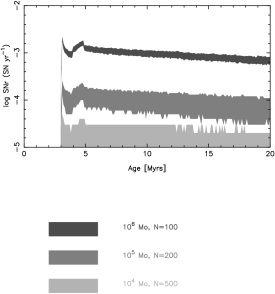
Figure 3: 90% Confidence limit from Monte Carlo simulations for the SNr of clusters with different amount of total mass transformed into stars since the beginning of the burst of star formation with a time step of 0.1 Myr

The dispersion obtained from the Monte Carlo simulations is given by $\sigma_{Mon}$ = SNr(t) x $\Delta t$. This time-dependence in the dispersion must be taken into account for quantities related to the SNr. Note that the obtained dispersion is correct if the SNr is defined in units of number of SN each $10^{5}$ years instead the usual units of SN per year.

As an example, it is assumed that our Galaxy have a mean SNr about 3 SNe per century which means, assuming a Poissonian distribution for the SNr, $\sigma_{SNr}\sim 2$ SN per century and a relative dispersion of 0.6. If the SNr is defined as 3 10⁴ SN per Myr, the corresponding $\sigma_{SNr}$ becomes 173 SN per Myr and the relative dispersion is 0.006.

4 Kinetic energy and ejected masses

The kinetic energy and ejected masses have two components: stellar winds and SNe. As we have pointed out before, all the outputs are affected by the way the interpolations are performed in the $\log M-\log t_{k}$ plane. In the following we use parabolic interpolations in this plane. Note that such interpolations produce a bit lower life-time that linear ones, which means a lower amount of kinetic energy and integrated ejected masses. We now study these properties in more detail.

We assume a typical value of 10⁵¹ erg SNe^-1 for the kinetic energy released by a SN. The kinetic power, $P_{kin}(t)$, is the product of the typical energy released by a SN multiplied by the $SNr(t)$. In the case of ejected masses, we need to use a relation between the SN ejected masses and the mass of the exploding star. Illustrative examples can be found in Portinari et al. (1998) and Cerviño et al. (2000a).

4.1 Stellar wind components

The kinetic energy and ejected masses also include a contribution from stellar winds. The stellar mass-loss rate is the key parameter needed to compute the kinetic energy and the ejected masses from stars before the end of their evolution. The total kinetic power is the sum over the contribution of individual stars, $p_{i}(t)$ at age $t$:

$$P_{kin}(t)=\sum_{i}^{N}w_{i}p_{i}(t)=\frac{1}{2}\sum_{i}^{N}w_{i}\dot{m_{i}}(t)v^{2}_{\infty,i}(t),$$ (13)

where $\dot{m_{i}}(t)$ is obtained from interpolations of the tracks and $v_{\infty,i}(t)$ is derived from the interpolated luminosity, the effective temperature, the mass $m_{i}$, and the metallicity of the star of initial mass $M_{i}$ at the given age, following Leitherer and Heckman (1995).

Similarly, the instantaneous ejected mass of an element $z$, $\dot{y_{z}}(t)$, can be computed as:

$$\dot{y}_{z}(t)=\sum_{i}^{N}w_{i}\dot{y}_{z,i}(t)=\sum_{i}^{N}w_{i}\dot{m_{i}}(t)Z_{i}(t),$$ (14)

where $Z_{i}$ is the mass fraction of the surface abundance of the element $z$ for a star of initial mass $M_{i}$ at age $t$. In general, in evolutionary synthesis codes, interpolations in $L$, $T_{eff}$, $\dot{m}$ and $m$ are performed in the $\log M-\log A_{k}$ plane, and those in $Z$ in the $\log M-Z_{k}$ plane, where the subindex $k$ refers to a given evolutionary stage. In the case of chemical evolution models the interpolations in $Z$ vary for different authors, from linear interpolations in the $M-Z$ plane (Ferrini et al. 1994) to the use of splines (Carigi 2000).

For the computation of the corresponding time integrated quantities — the cumulative kinetic energy $E_{kin}$ and the total yield $y_{z}$ — an additional sum over time is needed. Two different approximations may be followed:

• Method (a) The results from previous computed ages are used to compute the sum: Each value of $P_{kin}(t_{j})$ or $\dot{y}_{z}(t_{j})$ can be considered constant over the time interval between $t_{j-1}$ and $t_{j}$, where the index $j$ defines the age array used for the code output, and the $E_{kin}$ and $y_{z}$ are obtained adding up such contributions. Note that this method depends on the age array used and will lose evolutionary stages where the characteristic time is shorter than the time step used.

• Method (b): A similar treatment to those of chemical evolution models is used. An additional table for each evolutionary state, $k$, with the integrated amount of kinetic energy or chemical abundances from $t=0$ to each tabulated age, $t_{k}$ is computed. The final point of the table is the integrated energy and ejected mass resulting from the action of stellar winds all along the evolution of the star.

  This method has two possible implementations:

  • Method (b.1): The kinetic energy or chemical abundances tables are obtained using the mass-loss, i.e. for the chemical abundances case:

    $$y_{z,i}(t_{k^{\prime}})=\sum_{k=1}^{k^{\prime}}\dot{m_{i}}(t_{k})\,Z_{i}(t_{k})\,(t_{i,k}-t_{i,k-1}),$$ (15)

    where the subindex $k$ refers to the tabulated points in the tracks for the star of initial mass $M_{i}$.

  • Method (b.2): The instantaneous mass is used instead of the mass loss:

    $$y_{z,i}(t_{k^{\prime}})=\sum_{k=1}^{k^{\prime}}[m_{i}(t_{k})-m_{i}(t_{k-1})]\,<Z_{i}(t_{k})>,$$ (16)

    where $<Z_{i}(t_{k})>$ is the mean value of the surface abundance at the evolutionary ages $t_{k}$ and $t_{k-1}$ of a star of initial mass $M_{i}$. This is the approximation we have used here.

  In both cases, the total amount of the ejected element $z$ at a given age $t$ becomes:

  $$y_{z}(t)=\sum_{i=1}^{N}w_{i}y_{z,i}(t)$$ (17)

  This method has the advantage that the output does not depend on the age array used in the synthesis code.

The three methods should converge to the same value, but this can be only achieved if the time step used in method (a) is the same as the lowest time step used in the evolutionary tracks (i.e. a few years, that it is prohibitive for realistic computations). Methods (b.1) and (b.2) must also converge if

$$\dot{m_{i}}(t_{k})\,(t_{i,k}-t_{i,k-1})=m_{i}(t_{k})-m_{i}(t_{k-1}),$$ (18)

which is, however, not found to be true for various sets of stellar tracks adopted.

Let us illustrate the situation defining the ratio $R$ for each star as:

$$R=\frac{\sum_{k=1}^{k_{e}}\dot{m}(t_{k})\,(t_{k}-t_{k-1})}{M-m_{k_{e}}}$$ (19)

where the index $k_{e}$ refers to the last tabulated point in the track. Such ratio must be equal to 1 if Eq. 18 is fulfilled. The resulting values are shown in Fig. 4 and in Table 2 for the Schaller et al. (1992) tracks at solar metallicity and standard mass-loss rate and Meynet et al. (1994) tracks at twice solar metallicity and twice mass-loss rate.

Figure 4: Ratio of the integrated mass-loss during the lifetime of the star vs. “reconstructed” mass loss by subtraction of the mass at the Zero Age Main Sequence (ZAMS) and the mass at the end of the evolution for Schaller et al. (1992) tracks (solid line) at solar metallicity and standard mass-loss rate and Meynet et al. (1994) tracks at twice solar metallicity and twice mass-loss rate tracks (dashed line).

Initial	$\sum\dot{m}\Delta t$	$M-m_{k_{e}}$	$\sum\dot{m}\Delta t$	$M-m_{k_{e}}$
Mass range	(b.1)	(b.2)	(b.1)	(b.2)
(M⊙)	Z⊙		2xZ⊙, 2x$\dot{M}$
12	0.5	0.4	2.3	2.3
15	1.5	1.4	3.5	3.5
20	3.6	3.5	10.1	9.8
25	9.6	9.4	18.6	19.3
40	31.3	31.9	33.0	35.5
60	47.6	52.2	63.3	56.2
85	68.3	76.0	83.8	82.5
120	129	112	120	118

Table 2: Values of the mass loss between the ZAMS and the end of the evolution, and the integrated mass loss during the lifetime for different mass ranges from the Schaller et al. (1992) solar metallicity tracks and Meynet et al. (1994) tracks at twice solar metallicity and twice mass-loss rate.

Typically, as shown in Fig. 4 and Table 2 the ratio $R$ between the “reconstituted” integrated mass loss using the above methods and the total mass loss given by the difference between the tabulated initial and final mass of the tracks, is found to vary by up to $\sim$ 10 % for stars with non negligible mass loss. Note that for a 120 M_⊙ star the integrated mass loss is equal or higher than the initial mass!

4.2 Global evolution and dispersion

We now study the resulting integrated kinetic energy and chemical yields including both stellar winds and SNe. As an example, we have focused on the ejected mass of ¹²C and ¹⁴N/¹²C ratio. These elements, principally ¹⁴N, in a ”standard” stellar population are mostly produced by the intermediate stars in the Asymptotic Giant Branch (AGB) phase and when they form Planetary Nebulae (PNe). However AGB stars and PNe appear at later ages than those discussed in our work. Therefore, the ¹⁴N and ¹²C produced in the first few Myr come only from massive stars through stellar winds and SN explosions. We have selected these two elements as illustrative examples, to highlight the importance of the WR-wind phase in massive stars.

Figure 5: Top: Integrated kinetic energy using three different time steps with method (a) and using method (b.2) described in the text with interpolations in the $M-E_{kin}$ plane (linear) and $\log M-\log E_{kin}$ plane (log – log). Bottom: $N_{\mathrm{eff}}(E_{kin})$ as defined in Eq. 11 and computed by method (b.2) using the $M-E_{kin}$ plane for interpolations. The right vertical axis shows the minimum amount of gas that needs to be transformed into stars (in the given mass range and for the given IMF slope) to give a relative dispersion lower than 10% when analytical-IMF models are compared with real data.

Figure 6: Integrated amount of ¹²C ejected using three different time steps with method (a) and using method (b.2) described in the text with interpolations in the $M-^{12}$C plane (linear) and $\log M-\log^{12}$C plane (log – log). Bottom: $N_{\mathrm{eff}}(^{12}\mathrm{C})$ from method (b.2) using the $M-C$ plane for interpolations. The right vertical axis shows the minimum amount of gas that needs to be transformed into stars (in the given mass range and for the given IMF slope) to give a relative dispersion lower than 10% when analytical-IMF models are compared with real data.

Figures 5, 6 and 7 show these quantities computed with method (a) for various time steps $\Delta t$, and using method (b.2) with different interpolation techniques. For method (a) we use linear interpolations in $\log M-A$ for the abundances, and $\log M-\log A$ for $E_{kin}$. For method (b.2) we compare linear interpolations in the $M-A$ and $\log M-\log A$ planes. The examination of the figures shows the following: i) time steps $\la$ 0.1 Myr using method (a) appear adequate to properly calculate the considered quantities; ii) at young ages dominated by stellar winds ($t\la$ 3 Myr), the use of pretabulated integrated quantities (method b) leads to a somewhat larger and more correct values for kinetic energy and yields produced by massive stars. The origin of this difference is due to rapid variations of these quantities along the isochrone, which are not well enough resolved by method (a). The differences between the different numerical techniques are relevant for the younger ages, when the integration of stellar winds are the only contribution of the time-integrated quantities. Using method (a) our code needs about 30’ of CPU time in a SunOS sparc machine using a time step of 0.1 Myr form 0.1 to 20 Myr. The CPU time is in this case inversely proportional to the time step, i.e. the code would require about 300’ of CPU time to obtain very similar results once the SN activity is the dominant source, with a time step of 0.01 Myr. On the other hand, the time computations by method (b.2) are not time-step dependent and they produce stable results whatever the time step is.

In the lower panel of Fig. 5, 6 and 7 we show the resulting $N_{\mathrm{eff}}$ for the kinetic energy and ejected masses resulting from method (b.2) using interpolations in the $M-A$ plane. $N_{\mathrm{eff}}$ can be easily computed for the integrated properties if method (b.2) is used. Note, though, that the evaluation $N_{\mathrm{eff}}$ of the integrated properties from method (a) with a dynamical mass binning is quite difficult because we need to know the contribution of the same individual population along all the computed ages.

In the case of the kinetic energy, the relative dispersion decreases with age once the first SNe appears in the cluster. The natural explanation is that more and more stars contribute to the released kinetic energy and the statistics becomes better and better.

For the ¹²C case, there are three dominant contributions at different times: massive non-WR stellar winds from 0 to 3 Myr, WR stellar winds from 3 to 5 Myr and the SNe thereafter. The depression in $N_{\mathrm{eff}}(^{12}\mathrm{C})$ at 3 Myr coincides with the onset of the WR phase. As it has been shown in Paper ii, the WR phase is strongly influenced by the discreteness of the stellar population and shows a high dispersion in the related properties. The cumulative production of ¹²C by SNe decreases again the dispersion after 5 Myr.

Figure 7: Top left: ¹⁴N/¹²C ratio obtained from the ejected ¹⁴N and ¹²C computed for three different time steps with method (a) and using method (b.2) described in the text with interpolations corresponding to Fig. 6. Bottom left: Detail of ¹⁴N/¹²C ratio obtained at the beginning of the burst of star formation. Top right: $N_{\mathrm{eff}}(^{14}\mathrm{N}/^{12}\mathrm{C})$ (see text). The right vertical axis shows the minimum amount of gas that needs to be transformed into stars (in the given mass range and for the given IMF slope) to give a relative dispersion lower than 10% when analytical-IMF models are compared with real data. Bottom right: Correlation coefficient, $\rho$(¹⁴N/¹²C).

The ¹⁴N/¹²C ratio (Fig. 7, left panels) shows several interesting effects. It is characterized by an increasing ratio until 3 Myr due to the effects of stellar winds of massive stars. WR stars start to appear in the cluster at about 2 Myr. The evolution of WR stars at solar metallicity follows the sequence of WR stars with N in the envelope (WN phase, characterized by a strong mass-loss rate) and a posterior WC phase, where C appears at the surface in an amount larger than N, with a mass-loss rate dependent on the mass of the WR (i.e. decreasing with time). The prevalence of massive OB stars and the WN phase last until 3 Myr and produce more N than C. Later the action of WC winds and SNe increases the C production.

The top right panel of Fig. 7 shows the evolution of $N_{\mathrm{eff}}(^{14}\mathrm{N}/^{12}\mathrm{C})$. The relative dispersion (inverse of $N_{\mathrm{eff}}$) reaches a minimum value during the WR phase as for ${}^{12}\mathrm{C}$. $N_{\mathrm{eff}}$ increases from the first SN explosion to 5 Myr, and it decreases again slowly for more evolved ages. The computation of $N_{\mathrm{eff}}(^{14}\mathrm{N}/^{12}\mathrm{C})$ must take into account the effect of the covariance (i.e. the correlation coefficient, $\rho(^{14}\mathrm{N}/^{12}\mathrm{C})$). Due to correlation effects, the dispersion in the ¹⁴N/¹²C ratio is lower than the dispersion on ¹²C or ¹⁴N alone. Note also that the dispersion of the ¹⁴N/¹²C ratio increases as the cluster evolves.

Finally Fig. 8 shows the resulting values of $E_{kin}$ and ${}^{14}\mathrm{N}/^{12}\mathrm{C}$ ratio from a set of Monte Carlo simulations. The figure shows the 90% confidence level for simulations where different amounts of gas have been transformed into stars. The exact values of the 90% confidence level can not be achieved by the numerical formulation proposed, as far as the corresponding probability density distributions are not known, but it is clear that the dispersion in the simulations have a similar behavior than the one obtained by the computation of $N_{\mathrm{eff}}$. In particular, Monte Carlo simulations and the computation of $N_{\mathrm{eff}}(^{14}\mathrm{N}/^{12}\mathrm{C})$ show that the dispersion in the ${}^{14}\mathrm{N}/^{12}\mathrm{C}$ ratio increases with age.

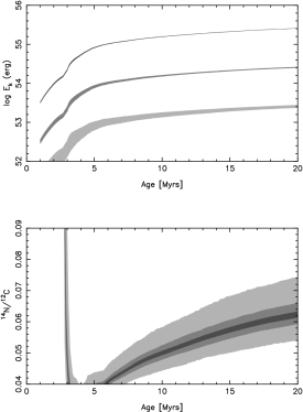
Figure 8: 90% Confidence level of Monte Carlo simulations for $E_{kin}$ and ${}^{14}\mathrm{N}/^{12}\mathrm{C}$ ratio of clusters with different amount of total mass transformed into stars since the beginning of the burst of star formation. The grey scale values are the ones defined in Fig. 3

5 Conclusions

We have discussed technical issues (accuracy, impact of various interpolation and integration methods) regarding the calculation of supernova rates, as well as chemical and mechanical yields in evolutionary synthesis models. Furthermore we have quantified the expected dispersion of these quantities due to stochastic effects in populations of various total masses. The main conclusions are the following:

1. Linear interpolations in the $\log M-\log t_{k}$ plane, where $M$ is the initial mass and $t$ is the age for a given evolutive stage, can give unphysical results for the supernova rate in particular and for the evolutionary phases in general

   A parabolic interpolation technique can improve the results, but a more general technique, taking into account the stellar evolution theory (i.e. the relation of the stellar evolution parameters like luminosity and effective temperature with time) would be an asset. However, as far as stellar theory is not complete, parabolic interpolations can be used to produce more reasonable results than linear ones.

   The unphysical results produced by the linear interpolations do not only affect the massive stars (as naively expected), but also the low mass ones (at least down to 9 M_⊙). The effects must be quantified for a wide age range, including low mass stars, in the evolutionary synthesis models.

2. The time-integrated quantities of instantaneous burst models (or single stellar populations) depend on the time step used for the integrations. For the quantities considered here a time step not larger than $\sim$ 0.1 Myr is found to be required for the integration of the stellar winds component, that are relevant at the early phases of the evolution of the cluster. However, the best choice in terms of computing time and accuracy is the use of predefined tables with the corresponding time-integrated quantities.

3. In early phases ($t\la$ 3 Myr) the kinetic energy and the ejected elements of star forming regions depend very strongly on the stellar winds. In these phases, the most accurate outputs are obtained when time-integrated tables of evolutionary tracks are used.

4. The discreteness of the real stellar populations is expected to produce a dispersion in the observed parameters that must be taken into account a priori when compared to the outputs of synthesis models. For time-integrated quantities, the dispersion is higher at the beginning of the star formation episode and becomes even more important during the WR phase. The dependence of the theoretical dispersion on the total stellar mass has been quantified.

5. When the correlation between different yields of elements is taken into account, the dispersion of the ratio of such elements increases with time. The relevance of this effect on the observed dispersion of the ${}^{14}\mathrm{N}/^{12}\mathrm{C}$ ratio remains to be evaluated.