Implications of O and Mg abundances in metal-poor halo stars
for stellar iron yields

Inhomogeneous chemical evolution models of galaxies which try to reproduce the scatter seen in element-to-iron ratios of metal-poor halo stars are heavily dependent on theoretical nucleosynthesis yields of core-collapse supernovae (SNe II). Hence inhomogeneous chemical evolution models present themselves as a test for stellar nucleosynthesis calculations. Applying such a model to our Galaxy reveals a number of shortcomings of existing nucleosynthesis yields. One problem is the predicted scatter in [O/Fe] and [Mg/Fe] which is too large compared to the one observed in metal-poor halo stars. This can be either due to the oxygen or magnesium yields or due to the iron yields (or both). However, oxygen and magnesium are $\alpha$-elements that are produced mainly during hydrostatic burning and thus are not affected by the theoretical uncertainties afflicting the collapse and explosion of a massive star. Stellar iron yields, on the other hand, depend heavily on the choice of the mass-cut between ejecta and proto-neutron star and are therefore very uncertain. We present iron yield distributions as function of progenitor mass that are consistent with the abundance distribution of metal-poor halo stars and are in agreement with observed $\@element[56]{\mathrm{Ni}}$ yields of core-collapse supernovae with known progenitor masses. The iron yields of lower-mass SNe II (in the range $10-20\,\mathrm{M}_{\sun}$) are well constrained by these observations. Present observations, however, do not allow us to determine a unique solution for higher-mass SNe. Nevertheless, the main dependence of the stellar iron yields as function of progenitor mass can be derived and may be used as a constraint for future core-collapse supernova/hypernova models. A prediction of hypernova models is the existence of ultra $\alpha$-element enhanced stars at metallicities [Fe/H] $\leq-2.5$, which can be tested by future observations. The results are of importance for the earliest stages of galaxy formation when the ISM is dominated by local chemical inhomogeneities and the instantaneous mixing approximation is not valid.

1 Introduction

The key to the formation and evolution of the Galaxy lies buried in the kinematic properties and the chemical composition of its stars. Especially old, metal-poor halo stars and globular clusters are ideal tracers of the formation process. Although many of the properties of the halo component and its substructures have been unveiled, it is still not possible to decide whether the Galaxy formed by a fast monolithic collapse (Eggen, Lynden-Bell & Sandage, els62 (1962)), by the slower merging and accretion of subgalactic fragments (Searle & Zinn sz78 (1978)) or within the context of a hybrid picture, combining aspects of both scenarios. Recently, Chiba & Beers (cb00 (2000)) made an extensive investigation to address this question, concluding that a hybrid scenario, where the inner part of the halo formed by a fast, dissipative collapse and the outer halo is made up of the remnants of accreted subgalactic fragments, best explains the observational data. It also seems to be consistent with the theory of galaxy formation based on cold dark matter scenarios (see e.g. Steinmetz & Müller sm95 (1995); Gnedin gn96 (1996); Klypin et al. kl99 (1999); Moore et al. mo99 (1999); Pearce et al. pe99 (1999); Bekki & Chiba bc00 (2000); Navarro & Steinmetz na00 (2000)).

However, the kinematic structure of the halo alone is not sufficient to draw a conclusive picture of the formation of the Galaxy. Old, unevolved metal-poor halo stars allow us to probe the chemical composition and (in)homogeneity of the early interstellar medium (ISM) and its evolution with time, since element abundances in the stellar atmospheres of those stars directly reflect the chemical composition of the material out of which they formed. It is almost impossible to determine the age of single stars (except in a few cases where radioactive thorium or uranium was detected, see e.g. Cayrel et al. cy01 (2001)). Therefore, the metallicity $Z$ or iron abundance [Fe/H] of a star is taken as an age estimate, knowing that an age–metallicity relation can only be used in a statistical sense for the bulk of stars (see e.g. Argast et al. ar00 (2000), hereafter Paper I).

Common chemical evolution models mostly assume that the metal-rich ejecta of supernovae (SNe) are mixed instantaneously and homogeneously into the ISM. Models using this approximation, together with theoretical nucleosynthesis yields of type Ia and type II SNe, can explain the behaviour of element-to-iron ratios ([el/Fe]) of stars as function of metallicity [Fe/H] for many elements and for [Fe/H] $\geq-2$. This shows that the instantaneous mixing approximation is valid at this stage and – since at these metallicities even some of the lowest mass core-collapse supernovae (SNe II) have exploded – that the stellar yields averaged over the initial mass function (IMF) are for most elements accurate within a factor of two (see e.g. Samland sa97 (1997)).

However, observations of very metal-poor stars show significant scatter in [el/Fe] ratios at [Fe/H] $<-2$, implying that the ISM was not well mixed at this stage (Paper I). These local chemical inhomogeneities were probably mainly caused by SNe II, since progenitors of SN Ia have much longer lifetimes and are unimportant for the chemical enrichment of the ISM until approximately [Fe/H] $\geq-1$. At these early stages of galaxy formation, the instantaneous mixing approximation is not valid and yields depending on the mass of individual SNe II become important. Therefore, accurate nucleosynthesis yields as a function of progenitor mass are crucial for the understanding of the earliest stages of galaxy formation.

In Paper I, a stochastic chemical evolution model was presented which accounts for local chemical inhomogeneities caused by SNe II with different progenitor masses. The model successfully reproduces the scatter in [el/Fe] ratios as function of [Fe/H] for some elements like Si or Ca, but fails quantitatively in the case of the two most abundant $\alpha$-elements, O and Mg. The scatter in [O/Fe] and [Mg/Fe] is much larger than observed and predicts stars with [O/Fe] and [Mg/Fe] $\leq-1.0$. This result depends mainly on the employed stellar yields, demonstrating that either the oxygen/magnesium or the iron yields (or both) as a function of progenitor mass are not well determined by existing nucleosynthesis models.

The solution to this problem is important for the understanding of the chemical evolution of our Galaxy. In this work, we try to reconcile element abundance observations of metal-poor halo stars with the predictions of our inhomogeneous chemical evolution model by changing the progenitor mass dependence of stellar yields. The formation of oxygen and magnesium in hydrostatic burning and ejection during a SN event is much better understood than the formation and ejection of $\@element[56]{\mathrm{Ni}}$ (which decays to $\@element[56]{\mathrm{Fe}}$ and forms the bulk of the ejected iron), since the amount of ejected $\@element[56]{\mathrm{Ni}}$ is directly linked to the still not fully understood explosion mechanism (c.f. Liebendörfer et al. li01 (2001); Mezzacappa et al. me01 (2001); Rampp & Janka ra00 (2000)). Any attempt to alter stellar yields should therefore start with iron and iron-group elements. We present a method to derive stellar iron yields as function of progenitor mass from the observations of metal-poor halo stars, assuming given yields of oxygen and magnesium.

In Sect. 2 we give a short description of the stochastic chemical evolution model, followed by a summary of observations and basic model results in Sect. 3. The discussion of uncertainties in stellar yields and how global constraints on stellar iron yields can be gained from observations is given in Sect. 4. Implications for stellar iron yields and conclusions are given in Sect. 5 and Sect. 6, respectively.

2 The chemical evolution model

Observations of very metal-poor halo stars show a scatter in [el/Fe] ratios of order 1 dex. This scatter gradually decreases at higher metallicities until a mean element abundance is reached which corresponds to the [el/Fe] ratio of the stellar yields integrated over the initial mass function. Our stochastic chemical evolution model of Paper I follows the enrichment history of the halo ISM in a cube with a volume of (2.5 kpc)³, down to a resolution of (50 pc)³. Every cell of the grid contains detailed information about the enclosed ISM and the mass distribution of stars. For the purpose of this paper, the enrichment of the ISM with O, Mg, Si, Ca and Fe is computed.

At every time-step, randomly chosen cells may create stars. The likelihood for a cell to form a star is proportional to the square of the local ISM density. The mass of a newly formed star is chosen randomly, with the condition that the mass distribution of all stars follows a Salpeter IMF. The lower and upper mass limits for stars are taken to be $0.1\,\mathrm{M}_{\sun}$ and $50\,\mathrm{M}_{\sun}$, respectively. Newly born stars inherit the abundance pattern of the ISM out of which they formed, carrying therefore information about the chemical composition of the ISM at the place and time of their birth.

Stars in a range of $10-50\,\mathrm{M}_{\sun}$ are assumed to explode as SNe II (or hypernovae, we will use the term SNe II to include hypernovae unless otherwise noted) resulting in an enrichment of the neighbouring ISM. Intermediate mass stars form planetary nebulae, which return only slightly enriched material. Low mass stars do not evolve significantly during the considered time but serve to lock up part of the mass, affecting therefore the abundances of elements with respect to hydrogen. Stellar yields are taken from Thielemann et al. (th96 (1996), hereafter TH96) and Nomoto et al. (no97 (1997)). Additionally, since there are no nucleosynthesis calculations for $10\,\mathrm{M}_{\sun}$ progenitors, their yields were set to $1/10$ of the yields of the $13\,\mathrm{M}_{\sun}$ model. We then linearly interpolated the stellar yields given in these papers, since we use a finer mass-grid in our simulation. The interpolation gives IMF averaged values of [el/Fe] ratios which are in good agreement (within 0.1 dex) with the observed mean values of metal-poor stars.

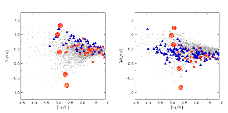
Figure 1: [O/Fe] and [Mg/Fe] ratios vs. metallicity [Fe/H] of metal-poor halo stars (squares and triangles) and model stars (dots). Circles depict [O/Fe] and [Mg/Fe] ratios of SN II models of the given progenitor mass. (See text for details.) In contrast to observations, model stars with subsolar [O/Fe] and [Mg/Fe] ratios are predicted by the applied stellar yields, as visible by the location of the 13 and 15 M_☉ SNe.

The SN remnant sweeps up the enriched material in a spherical, chemically well mixed shell. Since the explosion energy of SNe II is believed to depend only slightly on the mass of its progenitor (Woosley & Weaver ww95 (1995), hereafter WW95; Thielemann et al. th96 (1996)), we assume that each SN II sweeps up about $5\times 10^{4}\,\mathrm{M}_{\sun}$ of gas (Ryan et al. ry96 (1996); Shigeyama & Tsujimoto sh98 (1998)). Stars which form out of material enriched by a single SN inherit its abundance ratios and therefore show an element abundance pattern which is characteristic for this particular progenitor mass. This will lead to a large scatter in the [el/Fe] ratios, as long as local inhomogeneities caused by SN events dominate the halo ISM. As time progresses, supernova remnants overlap and the abundance pattern in each cell approaches the IMF average, leading to a decrease in the [el/Fe] scatter at later times. Since the SN remnant formation is the only dynamical process taken into account, this model shows the least possible mixing efficiency for the halo ISM. This is just the opposite to chemical evolution models which use the instantaneous mixing approximation. We continue our calculation up to an average iron abundance of [Fe/H] $=-1.0$. At this metallicity, SN Ia events which are not included in our model start to influence the ISM significantly. A more detailed description of the model can be found in Paper I.

We emphasize one important result: Starting with a primordial ISM and taking into account local inhomogeneities caused by SNe II, the initial scatter in [el/Fe] ratios is determined solely by the adopted nucleosynthesis yields. The details of the chemical evolution model only determine how fast a chemically homogeneous ISM is reached, i.e. how the scatter evolves with time or (equivalently) iron abundance [Fe/H]. Therefore, the range of [el/Fe] ratios of the most metal-poor stars does not depend on specific model parameters but is already fixed by the stellar yields.

3 Observations and basic model results

As mentioned in the introduction, existing nucleosynthesis models, combined with a chemical evolution model taking local inhomogeneities into account, predict [O/Fe] and [Mg/Fe] ratios less than solar for some metal-poor stars. This is in contrast to observations of metal-poor halo stars, as can be seen in Fig. 1. The left hand panel shows the [O/Fe] ratio of observed and model stars as function of iron abundance [Fe/H] and the right hand panel the same for [Mg/Fe], where the model stars are plotted as small dots. The observational data were collected from Magain (ma89 (1989)), Molaro & Bonifacio (mb90 (1990)), Molaro & Castelli (mc90 (1990)), Peterson et al. (pe90 (1990)), Bessell et al. (be91 (1991)), Ryan et al. (ry91 (1991)), Spiesman & Wallerstein (sw91 (1991)), Spite & Spite (sp91 (1991)), Norris et al. (no93 (1993)), Beveridge & Sneden (be94 (1994)), King (ki94 (1994)), Nissen et al. (ni94 (1994)), Primas et al. (pr94 (1994)), Sneden et al. (sn94 (1994)), Fuhrmann et al. (fu95 (1995)), McWilliam et al. (mw95 (1995)), Balachandran & Carney (ba96 (1996)), Ryan et al. (ry96 (1996)), Israelian et al. (is98 (1998)), Jehin et al. (je99 (1999)), Boesgaard et al. (bo99 (1999)), Idiart & Thévenin (id00 (2000)), Carretta et al. (ca00 (2000)) and Israelian et al. (is01 (2001)).

Combining data from various sources is dangerous at best, since different investigators use different methods to derive element abundances with possibly different and unknown systematic errors. This influences the scatter in [el/Fe] ratios, which plays a crucial rôle in determining the chemical (in)homogeneity of the ISM as function of [Fe/H]. Unfortunately, there is no investigation with a sample of oxygen/magnesium abundances of metal-poor halo stars that is large enough for our purpose. Therefore, we are forced to combine different data sets, keeping in mind that unknown systematic errors can enlarge the intrinsic scatter in element abundances of metal-poor stars. Recently, Idiart & Thévenin (id00 (2000)) and Carretta et al. (ca00 (2000)) reanalyzed data previously gathered by other authors and applied NLTE corrections to O, Mg and Ca abundances, which is a first step in reducing the scatter introduced by systematic errors. Therefore we divided the collected data into two groups, namely the data of Idiart & Thévenin (id00 (2000)) and Carretta et al. (ca00 (2000)), which is represented in Fig. 1 by triangles, and the data of all other investigators, represented by squares. If multiple observations of a single star exist, abundances are averaged and pentagons and diamonds are used for the first and second group, respectively. (Averaging of data points was only necessary in a few cases for Mg, Si and Ca abundances.) Note, that the average random error in element abundances is of the order 0.1 dex.

Also plotted in Fig. 1 as circles are [el/Fe] ratios predicted by nucleosynthesis calculations of TH96. The numbers in the circles give the mass of the progenitor star in solar masses. In the picture of inhomogeneous chemical evolution, a single SN event enriches the primordial ISM locally (in our model by mixing with $5\times 10^{4}\,\mathrm{M}_{\sun}$ of ISM) with its nucleosynthesis products. Depending on the mass of the progenitor star, the resulting [O/Fe] and [Mg/Fe] ratios in these isolated patches of ISM cover a range of over two dex and as long as the ISM is dominated by these local inhomogeneities, newly formed stars will show the same range in their [el/Fe] ratios. In particular, this means that stars with [O/Fe] and [Mg/Fe] as small as $-1.0$ are inevitably produced by our model. This is in contrast to the bulk of observed metal-poor halo stars, which show [O/Fe] and [Mg/Fe] ratios in the range between 0.0 and 1.2, and is a strong indication that existing nucleosynthesis models may correctly account for IMF averaged abundances but fail to reproduce stellar yields as function of progenitor mass.

4 Global constraints on stellar Fe yields

4.1 Uncertainties in O, Mg and Fe yields

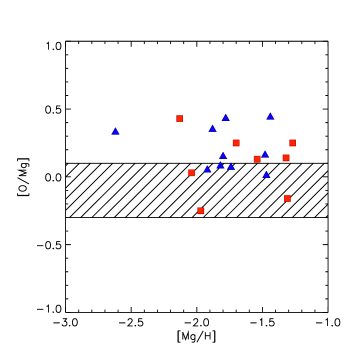
Figure 2: [O/Mg] vs. [Mg/H] ratios of metal-poor halo stars. Nucleosynthesis models predict a narrow region of possible [O/Mg] ratios (hatched) which is not consistent with the scatter of observations. Symbols are as in Fig. 1.

Apart from the shortcomings of nucleosynthesis yields discussed in Sect. 3, there seems to be an additional uncertainty concerning either the stellar yields of O and Mg or the derivation of their abundances in metal-poor halo stars, as shown in Fig. 2:

The theoretical nucleosynthesis yields of oxygen $\left(Y_{\mathrm{O}}\left(m\right)\right)$ and magnesium $\left(Y_{\mathrm{Mg}}\left(m\right)\right)$ show a very similar dependence on progenitor mass $m$, i.e. in first order we can write $Y_{\mathrm{Mg}}\left(m\right)\approx 6.7\cdot 10^{-2}\cdot Y_{\mathrm{O}}\left(m\right)$. Thus, for model stars [O/Mg] $\approx 0.0$ on average, and due to chemical inhomogeneities in the early ISM, model stars scatter in the range $-0.3\leq[$O/Mg$]\leq 0.1$ (hatched region in Fig. 2). In contrast to theoretical predictions, observations of metal-poor halo stars scatter in the range $-0.3\leq$ [O/Mg] $\leq 0.5$, with a mean of [O/Mg] $\approx 0.15$. This result is very important, since it means that either even our understanding of nucleosynthesis processes during hydrostatic burning is incomplete or that oxygen abundances at very low metallicities tend to be overestimated (or magnesium abundances underestimated).

The problem hinted at in Fig. 2 is also connected to the recent finding that the mean [O/Fe] ratio of metal-poor halo stars seems to increase with decreasing metallicity [Fe/H], whereas the mean [Mg/Fe] ratio seems to stay constant (see e.g. Israelian et al. is98 (1998), is01 (2001); Boesgaard et al. bo99 (1999); King ki00 (2000); but see also Rebolo et al. re02 (2002)). This result can not be explained by changes in the surface abundances due to rotation, since rotation tends to decrease the oxygen abundance in the stellar atmosphere, whereas magnesium abundances remain unaffected (Heger & Langer hl00 (2000); Meynet & Maeder me00 (2000)). However, the problem described with Fig. 2 would disappear, if the increase in [O/Fe] with decreasing metallicity is not real but due to some hidden systematic error. Then oxygen abundances would have to be reduced, resulting in a smaller scatter and lower mean in [O/Mg].

Regarding nucleosynthesis products, a crude argument shows that (at least in the non-rotating case) we should not expect a drastic change in the progenitor mass dependence of O and Mg yields: Oxygen and magnesium are produced mainly during hydrostatic burning in the SN progenitor and only a small fraction of the ejecta stems from explosive neon- and carbon-burning (see e.g. Thielemann et al. th90 (1990), th96 (1996)). Magnesium is to first order a product of hydrostatic carbon- and ensuing neon-burning in massive stars. The amount of freshly synthesized magnesium depends on the available fuel, i.e. the size of the C-O core after hydrostatic He burning, which also determines the amount of oxygen that gets expelled in the SN event. Thus, O and Mg yields as function of progenitor mass should be roughly proportional to each other. A very large mass loss during hydrostatic carbon burning could reduce the size of the C-O core and thus decrease the amount of synthesized magnesium for a given progenitor mass. This would result in a larger scatter of [O/Mg] ratios than indicated by the hatched region in Fig. 2. But the evolutionary timescale of carbon burning is very short indeed ($\approx 5.8\cdot 10^{3}$ yr for a $25\,\textrm{M}_{\sun}$ star, e.g. Imbriani et al. im01 (2001)), making a significant change in the structure of the C-O core unlikely.

Although the hydrostatic burning phases are thought to be well understood, one has to keep in mind that the important (effective) $\@element[12]{\mathrm{C}}$($\alpha$, $\gamma$)$\@element[16]{\mathrm{O}}$ reaction rate is still uncertain and that the treatment of rotation and convection may also influence the amount of oxygen and magnesium produced during hydrostatic burning. Recently, Heger et al. (he00 (2000)) showed that even in the case of slow rotation important changes in the internal structure of a massive star occur:

Rotationally induced mixing is important prior to central He ignition. After central He ignition, the timescales for rotationally induced mixing become too large compared to the evolutionary timescales, and the further evolution of the star is similar to the non-rotating case. Nevertheless, He cores of rotating stars are more massive, corresponding to He cores of non-rotating stars with about 25% larger initial mass. Furthermore, for a given mass of the He core, the C-O cores of rotating stars are larger than in the non-rotating case. At the end of central He burning, fresh He is mixed into the convective core, converting carbon into oxygen. Therefore, the carbon abundance in the core is decreased, whereas the oxygen abundance is increased. Unfortunately, no detailed nucleosynthesis yields including rotation have been published yet, but since the size of the He core is increased in rotating stars, at least changes in the yields of $\alpha$-elements have to be expected. (For a review of the changes in the stellar parameters induced by rotation see Maeder & Meynet ma00 (2000).)

Contrary to oxygen and magnesium which stem from hydrostatic burning, iron-peak nuclei are a product of explosive silicon-burning. Unfortunately, no self-consistent models following the main-sequence evolution, collapse and explosion of a massive star exist to date which would allow to determine reliably the explosion energy and the location of the mass-cut between the forming neutron star and the ejecta (Liebendörfer et al. li01 (2001); Mezzacappa et al. me01 (2001); Rampp & Janka ra00 (2000)). Therefore, nucleosynthesis models treat the mass cut usually as one of several free parameters and the choice of its value can heavily influence the abundance of ejected iron-group nuclei. For this reason, we feel that oxygen and magnesium yields of nucleosynthesis models are more reliable than iron yields, in spite of the uncertainties discussed above.

To illustrate this point we show a comparison of O and Mg yields ($Y_{\mathrm{O}}\left(m\right)$, $Y_{\mathrm{Mg}}\left(m\right)$, Fig. 3) and of Fe yields ($Y_{\mathrm{Fe}}\left(m\right)$, Fig. 4) of nucleosynthesis calculations (neglecting rotation) from different authors. The models of WW95 (solar composition “C” models) are marked by filled squares, TH96 by filled circles, Nakamura et al. (na01 (2001), $10^{51}$ erg models) by open squares and Rauscher et al. (rh02 (2002), “S” models) by open triangles. Upper points in Fig. 3 correspond to O yields, lower points to Mg yields. Apart from the dip visible in $Y_{\mathrm{Mg}}\left(m\right)$ of the WW95 models, the O and Mg yields of the different authors agree remarkably well. Chemical evolution calculations by Thomas et al. (to98 (1998)) show that WW95 underestimate the average Mg yield due to this dip. The minor differences between the models can mostly be attributed to different progenitor models prior to core-collapse, the employed $\@element[12]{\mathrm{C}}$($\alpha$, $\gamma$)$\@element[16]{\mathrm{O}}$ reaction rate, the applied convection criterion (e.g. Schwarzschild vs. Ledoux) and artificial explosion methods after core-collapse (e.g. piston vs. artificially induced shock wave). On the other hand, as visible in Fig. 4, $Y_{\mathrm{Fe}}\left(m\right)$ of the different authors differs by more than an order of magnitude for certain progenitor masses, which is mostly due to the arbitrary placement of the “mass-cut” between proto-neutron star and ejecta. In order to reconcile the results of the inhomogeneous chemical evolution model with observed [O/Fe] and [Mg/Fe] abundance ratios, it is therefore clearly preferable to artificially adjust $Y_{\mathrm{Fe}}\left(m\right)$ rather than $Y_{\mathrm{O}}\left(m\right)$ and $Y_{\mathrm{Mg}}\left(m\right)$.

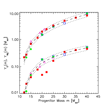
Figure 3: O and Mg yields from different authors as function of progenitor mass. Models are from: WW95, filled squares; TH96, filled circles; Nakamura et al. (na01 (2001)), open squares; Rauscher et al. (rh02 (2002)), open triangles. Upper points correspond to O yields, lower points to Mg yields. Dashed and dotted lines represent best fit curves to the different nucleosynthesis models (see text for details).

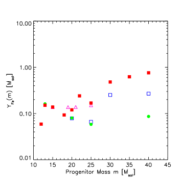
Figure 4: Fe yields from different authors as function of progenitor mass. Symbols are the same as in Fig. 3. Contrary to O and Mg yields, different authors obtain very different yields for a given progenitor mass. This is mostly due to the arbitrary placement of the mass cut.

For the following discussion, reliable O and Mg yields as function of progenitor mass with an estimate of their error range are needed. To this end, we calculated best fit curves to the $Y_{\mathrm{O}}\left(m\right)$ and $Y_{\mathrm{Mg}}\left(m\right)$ yields of the different authors, visible as dashed lines in Fig. 3. The low Mg yields of the 20 and 22 $\,\mathrm{M}_{\sun}$ WW95 models were neglected for this purpose. The deviations $\Delta\epsilon\left(m\right)$ of the original O and Mg yields $Y_{\mathrm{el}}\left(m\right)$ from our best fit yields $\overline{Y}_{\mathrm{el}}\left(m\right)$ is defined as

$$\Delta\epsilon\left(m\right)=\frac{Y_{\mathrm{el}}\left(m\right)-\overline{Y}_{\mathrm{el}}\left(m\right)}{\overline{Y}_{\mathrm{el}}\left(m\right)}.$$ (1)

The error $\Delta\epsilon\left(m\right)$ depends on progenitor mass, but is generally small. To account for the uncertainty in $Y_{\mathrm{el}}\left(m\right)$ introduced by the different nucleosynthesis models, we replace in the following the original $Y_{\mathrm{el}}\left(m\right)$ by $\left(1\pm\Delta\epsilon\right)\cdot\overline{Y}_{\mathrm{el}}\left(m\right)$, where we dropped the dependence of $\Delta\epsilon\left(m\right)$ on $m$ in the notation. For most progenitor masses, $\Delta\epsilon\leq 0.2$ for both O and Mg and the maximal deviation is in both cases smaller than 0.5. The dotted lines in Fig. 3 show the curves $\left(1\pm\Delta\epsilon\right)\cdot\overline{Y}_{\mathrm{el}}\left(m\right)$ with $\Delta\epsilon=0.2$. Since $\Delta\epsilon$ is small, the impact of the uncertainties in the stellar O and Mg yields is almost negligible for the derivation of constraints on $Y_{\mathrm{Fe}}\left(m\right)$. On the other hand, these small uncertainties may (almost) be able to explain the discrepancy in the scatter of [O/Mg] ratios between observations and model stars visible in Fig. 2. Allowing for a mean deviation of $\Delta\epsilon=0.2$, the maximal scatter in [O/Mg] over all progenitor masses may extend to $-0.25\leq$ [O/Mg] $\leq 0.3$, which is very close to the one observed. Future nucleosynthesis calculations have to show whether this interpretation is correct or not.

For the remaining discussion, we adopt the term $\left(1\pm\Delta\epsilon\right)\cdot\overline{Y}_{\mathrm{el}}\left(m\right)$ with $\Delta\epsilon=0.2$ for the stellar oxygen and magnesium yields as a function of progenitor mass, assuming that they reproduce the true production in massive stars well enough. The values adopted for the best fit yields $\overline{Y}_{\mathrm{el}}\left(m\right)$ are given in Table 1.

Table 1: Best fit O and Mg yields $\overline{Y}_{\mathrm{el}}\left(m\right)$ proposed in Sect. 4.1. The first column gives the progenitor mass $m$ and the following columns the oxygen and magnesium yields (all values in solar masses).

$m$	$\overline{Y}_{\mathrm{O}}\left(m\right)$	$\overline{Y}_{\mathrm{Mg}}\left(m\right)$	$m$	$\overline{Y}_{\mathrm{O}}\left(m\right)$	$\overline{Y}_{\mathrm{Mg}}\left(m\right)$
10	2.2E-02	1.2E-03	31	5.0E+00	3.3E-01
11	8.6E-02	4.9E-03	32	5.4E+00	3.5E-01
12	1.5E-01	8.5E-03	33	5.7E+00	3.6E-01
13	3.1E-01	2.0E-02	34	6.1E+00	3.8E-01
14	4.9E-01	3.6E-02	35	6.5E+00	4.0E-01
15	6.7E-01	5.3E-02	36	6.9E+00	4.2E-01
16	8.7E-01	6.9E-02	37	7.3E+00	4.4E-01
17	1.1E+00	8.6E-02	38	7.7E+00	4.5E-01
18	1.3E+00	1.0E-01	39	8.1E+00	4.7E-01
19	1.5E+00	1.2E-01	40	8.6E+00	4.9E-01
20	1.7E+00	1.4E-01	41	9.0E+00	5.2E-01
21	2.0E+00	1.5E-01	42	9.5E+00	5.4E-01
22	2.2E+00	1.7E-01	43	1.0E+01	5.6E-01
23	2.5E+00	1.9E-01	44	1.0E+01	5.9E-01
24	2.8E+00	2.0E-01	45	1.1E+01	6.1E-01
25	3.0E+00	2.2E-01	46	1.1E+01	6.4E-01
26	3.4E+00	2.4E-01	47	1.2E+01	6.6E-01
27	3.7E+00	2.6E-01	48	1.2E+01	6.8E-01
28	4.0E+00	2.7E-01	49	1.3E+01	7.1E-01
29	4.3E+00	2.9E-01	50	1.3E+01	7.3E-01
30	4.6E+00	3.1E-01

4.2 The influence of Z and SNe from Population III stars

Apart from the uncertainties in the O and Mg yields discussed in Sect. 4.1, nucleosynthesis yields may also depend on the metallicity of the progenitor. Unfortunately, the question how important metallicity effects are is far from solved. Nucleosynthesis calculations in general neglect effects of mass loss due to stellar winds. WW95 present nucleosynthesis results for a grid of metallicities from metal-free to solar and predict a decrease in the ejected O and Mg mass with decreasing metallicity. However, the O yields presented lie all in the range covered by the best fit yields $\left(1\pm\Delta\epsilon\right)\cdot\overline{Y}_{\mathrm{el}}\left(m\right)$ with $\Delta\epsilon=0.2$ adopted for this paper. This is not true in the case of Mg. But since the “dip” in $Y_{\mathrm{Mg}}\left(m\right)$ visible in Fig. 3 gets more and more pronounced with lower Z and since it is known (Thomas et al., to98 (1998)), that WW95 underestimate the average production of Mg, we feel that the metallicity dependence of Mg yields is not established well enough to include this feature into our analysis.

Contrary to the results obtained by WW95, Maeder (ma92 (1992)) showed that stellar O yields decrease with increasing metallicity due to strong mass loss in stellar winds. (No detailed results were given in the case of magnesium.) Stars more massive than $25\textrm{M}_{\sun}$ with solar metallicity (Z=0.02), eject large amounts of He and C in stellar winds (prior to the conversion into oxygen) which results in dramatically reduced O yields. Metal-poor stars (Z$\leq$0.001) do not undergo an extended mass-loss phase and their O yields are comparable to the ones given by WW95 and TH96. Since Z$\leq$0.001 roughly corresponds to [Fe/H] $\leq-1.5$ and we are mainly concerned with metal-poor halo stars in this metallicity range, we can neglect changes in O yields due to metallicity.

Recently, Heger & Woosley (hw01 (2000)) published nucleosynthesis calculations of pair-instability SNe from very massive, metal-free (Population III) stars in the mass range from $140\textrm{M}_{\sun}$ to $260\textrm{M}_{\sun}$. For Population III stars in the mass range $25-140\textrm{M}_{\sun}$ and stars more massive than $260\textrm{M}_{\sun}$, black hole formation without ejection of nucleosynthesis yields seems likely (Heger & Woosley hw01 (2000)). In order to investigate the influence of those massive metal-free stars on the enrichment of the ISM and especially their impact on the distribution of model stars in [O/Mg] vs. [Mg/H] plots (c.f. Sect. 4.1), we carried out several inhomogeneous chemical evolution calculations with varying SF efficiencies and IMF shapes for the Population III stars. The detailed results will not be shown here, but some basic conclusions are discussed in the following:

The theoretical scatter in [O/Mg] predicted by the massive Population III stars lies in the range $-0.3\leq$ [O/Mg] $\leq 0.3$. This could help to explain the scatter in [O/Mg] observed in metal-poor stars, if we take observational errors of the order of 0.1 dex into account. Models with a high SF efficiency for Population III stars indeed show some stars with high [O/Mg] ratios. However, 61% of the metal-poor stars ([Fe/H] $\leq-1.0$) with observed O and Mg abundances show [O/Mg] $\geq 0.1$ (see Fig. 2), whereas less than 1% of the model stars have [O/Mg] ratios in this range (the exact number depends on the shape of the IMF). Clearly, the observations of metal-poor stars can not be explained as a consequence of such massive, metal-free SNe. Furthermore, the distribution of model-stars in [O/Fe] and [Mg/Fe] can not be reconciled with observations of metal-poor stars. If the SF efficiency of Population III stars is small, these discrepancies in [O/Fe] and [Mg/Fe] disappear, but the number of model stars with [O/Mg] $\geq 0.1$ decreases even further. We therefore conclude that – at least for the purpose of this paper – the (possible) influence of SNe from very massive Population III stars can safely be neglected.

4.3 Putting constraints on Fe yields with the help of observations

In order to reproduce the scatter of observed [O/Fe] and [Mg/Fe] ratios of metal-poor halo stars while keeping the oxygen and magnesium yields fixed, we have to adjust the stellar iron yields $Y_{\mathrm{Fe}}\left(m\right)$ as function of progenitor mass $m$. Since it is not known from theory what functional form $Y_{\mathrm{Fe}}\left(m\right)$ follows (increasing with $m$, declining or a more complex behaviour), we have the freedom to make some ad hoc assumptions. Nevertheless, some important constraints on $Y_{\mathrm{Fe}}\left(m\right)$ can be drawn from the scatter, range and mean of observed [O/Fe] and [Mg/Fe] abundances, as visible from Fig. 1:

1. IMF averaged stellar yields (integrated over a complete generation of stars) should reproduce the mean oxygen and magnesium abundances of metal-poor halo stars, i.e. [O/Fe] $\approx 0.4$ and [Mg/Fe] $\approx 0.4$.

2. Stellar yields have to reproduce the range and scatter of [el/Fe] ratios observed. Using oxygen and magnesium as reference this requires:

   $$0.0\leq \mathrm{[O/Fe]} \leq 1.2,$$ (2)

   $$-0.1\leq \mathrm{[Mg/Fe]} \leq 1.2.$$ (3)

   (Note, that the error in abundance determinations is of order 0.1 dex.)

3. There exist a few Type II and Type Ib/c SN observations (1987A, 1993J, 1994I, 1997D, 1997ef and 1998bw) where the ejected $\@element[56]{\mathrm{Ni}}$ mass and the mass of the progenitor was derived by analyzing and modelling the light-curve (e.g. Suntzeff & Bouchet sb90 (1990); Shigeyama & Nomoto sh90 (1990); Shigeyama et al. sh94 (1994); Iwamoto et al. iw94 (1994), iw98 (1998), iw00 (2000); Kozma & Fransson ko98 (1998); Turatto et al. tu98 (1998); Chugai & Utrobin cu00 (2000); Sollerman et al. so00 (2000)). These observations give important constraints on $Y_{\mathrm{Fe}}\left(m\right)$ since they constrain the stellar yields for some progenitor masses, although they are not unambiguous (see Sect. 4.3.3).

4. Since observations of metal-poor halo stars show no clear trends in [Mg/Fe] with decreasing [Fe/H] we require that modified iron yields likewise do not introduce any skewness in the distribution of model stars. In the case of oxygen, it is not clear yet whether the apparent slope in [O/Fe] in recent abundance studies is real or due to some systematic errors (see Fig. 1 and Sect. 4.1).

It is clear that it is not possible to predict $Y_{\mathrm{Fe}}\left(m\right)$ unambiguously, since the information drawn from observations is afflicted by errors. We therefore do not attempt to find a solution which reproduces the observations perfectly, but try to extract the global properties of $Y_{\mathrm{Fe}}\left(m\right)$ needed to explain the behaviour of observed [el/Fe] ratios in metal-poor halo stars.

4.3.1 IMF averaged iron yields

Since the yields of TH96 were calibrated so that the first constraint is fulfilled, we require that the average iron yield of SNe II stays constant when we change the progenitor mass dependence of $Y_{\mathrm{Fe}}\left(m\right)$. Assuming a Salpeter IMF ranging from $0.1\,\mathrm{M}_{\sun}$ to $50\,\mathrm{M}_{\sun}$ and assuming that all stars more massive than $10\,\mathrm{M}_{\sun}$ turn into core-collapse SNe (or hypernovae, see e.g. Nakamura et al. na01 (2001)), a SN II produces on average $\left<\overline{Y}_{\mathrm{O}}\right>\approx\,1.9\,\mathrm{M}_{\sun}$ of oxygen, $\left<\overline{Y}_{\mathrm{Mg}}\right>\approx\,0.12\,\mathrm{M}_{\sun}$ of magnesium and $\left<Y_{\mathrm{Fe}}\right>\approx\,0.095\,\mathrm{M}_{\sun}$ of iron. Leaving the average oxygen and magnesium yields unchanged and modifying the stellar iron yields, we therefore always have to require that on average $\approx 0.095\,\mathrm{M}_{\sun}$ of iron are ejected per SN. Thus, $Y_{\mathrm{Fe}}\left(m\right)$ has to satisfy the following condition:

$$\left<Y_{\mathrm{Fe}}\right>=\frac{\int_{10}^{50}Y_{\mathrm{Fe}}\left(m\right)m^{-2.35}dm}{\int_{10}^{50}m^{-2.35}dm}\approx 0.095\,\mathrm{M}_{\sun}.$$ (4)

Note that the average [el/Fe] ratio of the model stars depends on the lower and upper mass limits of stars that turn into SNe II and their yields. If we raise the lower mass limit, the average oxygen yield of a SN will increase since many stars with a low oxygen yield no longer contribute to the enrichment of the ISM. The same is true for magnesium and iron and the combination of the new averaged yields may lead to slightly changed average [el/Fe] ratios. Since there are only a few SNe with large progenitor masses, changing the upper mass limit will have a very small influence on the average [el/Fe] ratios. For the remaining discussion, we will keep the lower and upper mass limits of SNe II fixed at $10\,\mathrm{M}_{\sun}$ and $50\,\mathrm{M}_{\sun}$, respectively.

4.3.2 Range and scatter of observations

The second constraint can be used to calculate the range that $Y_{\mathrm{Fe}}\left(m\right)$ has to cover. In our picture of inhomogeneous chemical evolution, we assume that the first SNe locally enrich the primordial ISM. Stars forming out of this enriched material therefore inherit the [el/Fe] ratios produced by these SNe which is determined in turn by the stellar yields $\overline{Y}_{\mathrm{el}}\left(m\right)$. (For the time being, we neglect the additional uncertainty hidden in the factor $\left(1\pm\Delta\epsilon\right)$.) Thus, for the first few generations of stars formed at the time the ISM is dominated by local chemical inhomogeneities, the following identity holds (with the exception of H and He where also the abundances in the primordial ISM have to be taken into account):

$$\mathrm{[el/Fe]} = \log\frac{N_{\mathrm{el},\star}/N_{\mathrm{Fe},\star}}{N_{\mathrm{el},\sun}/N_{\mathrm{Fe},\sun}}=\log\frac{M_{\mathrm{el},\star}/M_{\mathrm{Fe},\star}}{M_{\mathrm{el},\sun}/M_{\mathrm{Fe},\sun}}$$

$$= \log\frac{\overline{Y}_{\mathrm{el}}\left(m\right)/Y_{\mathrm{Fe}}\left(m\right)}{M_{\mathrm{el},\sun}/M_{\mathrm{Fe},\sun}},$$

where $N_{\mathrm{el},\sun}$ $\left(N_{\mathrm{el},\star}\right)$ is the number density of a given element el in the solar (stellar) atmosphere and $M_{\mathrm{el},\sun}$ $\left(M_{\mathrm{el},\star}\right)$ the corresponding mass fraction. (Solar abundances were taken from Anders & Grevesse ag89 (1989)). Now, let $\overline{Y}_{\mathrm{el}}\left(m\right)$ be either the stellar yields of oxygen or of magnesium and $\alpha$, $\beta$ the minimal and maximal [el/Fe] ratios derived from observations. Then the constraint gives:

$$\alpha\leq[\mathrm{el/Fe}]\leq\beta\qquad\Longleftrightarrow$$

$$\alpha\leq\log\frac{\overline{Y}_{\mathrm{el}}\left(m\right)/Y_{\mathrm{Fe}}\left(m\right)}{M_{\mathrm{el},\sun}/M_{\mathrm{Fe},\sun}}\leq\beta\qquad\Longleftrightarrow$$

$$\overline{Y}_{\mathrm{el}}\left(m\right)\cdot 10^{-\beta}\cdot\frac{M_{\mathrm{Fe},\sun}}{M_{\mathrm{el},\sun}} \leq Y_{\mathrm{Fe}}\left(m\right)$$

$$\leq \overline{Y}_{\mathrm{el}}\left(m\right)\cdot 10^{-\alpha}\cdot\frac{M_{\mathrm{Fe},\sun}}{M_{\mathrm{el},\sun}}.$$

Since the yields of oxygen and magnesium as function of progenitor mass are assumed to be known, we now have two sets of inequalities for the stellar iron yields. The first is derived from the minimal and maximal [O/Fe] ratios (Eq. 2):

$$8.37\cdot 10^{-3}\cdot\overline{Y}_{\mathrm{O}}\left(m\right)\leq Y_{\mathrm{Fe}}\left(m\right)\leq 1.33\cdot 10^{-1}\cdot\overline{Y}_{\mathrm{O}}\left(m\right),$$ (5)

and the second from the minimal and maximal [Mg/Fe] ratios (Eq. 3):

$$1.23\cdot 10^{-1}\cdot\overline{Y}_{\mathrm{Mg}}\left(m\right)\leq Y_{\mathrm{Fe}}\left(m\right)\leq 2.46\cdot\overline{Y}_{\mathrm{Mg}}\left(m\right),$$ (6)

where the uncertainty in the O and Mg yields given by the factor $\left(1\pm\Delta\epsilon\right)$ was neglected. Thus, for any given progenitor mass, $Y_{\mathrm{Fe}}\left(m\right)$ is only determined within a factor of 20 – 25 and further constraints are needed to derive a reliable iron yield.

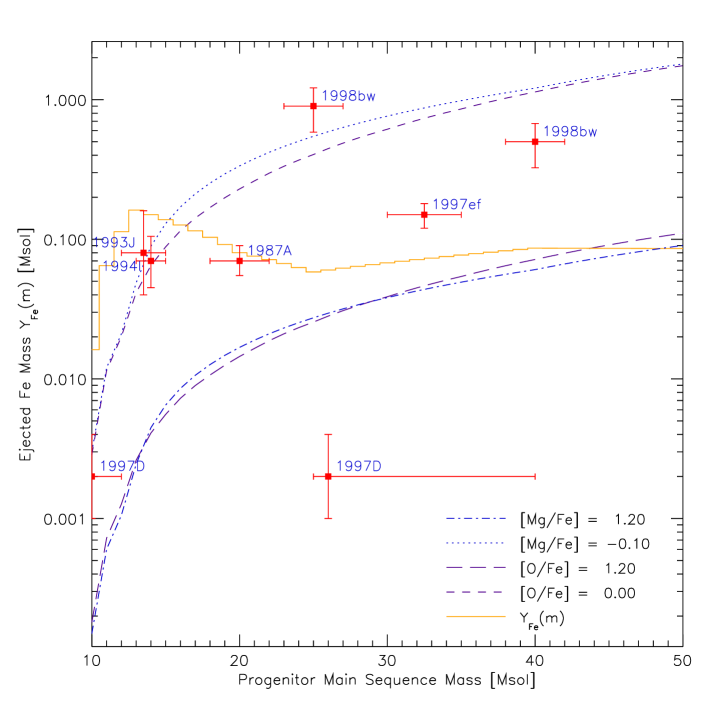
Figure 5: $Y_{\mathrm{Fe}}\left(m\right)$ as function of progenitor mass and boundaries constraining the range stellar iron yields have to satisfy to reproduce the scatter in [O/Fe] and [Mg/Fe] of metal-poor halo stars. According to nucleosynthesis models of Thielemann et al. (th96 (1996)) and Nomoto et al. (no97 (1997)), SNe in the range $10-15\,\mathrm{M}_{\sun}$ clearly eject too much iron to be consistent with observations. Also shown are observations of core-collapse SNe with known progenitor mass and ejected $\@element[56]{\mathrm{Ni}}$ mass.

Fig. 5 shows the stellar iron yields $Y_{\mathrm{Fe}}\left(m\right)$ (solid line) from Thielemann et al. (th96 (1996)) and Nomoto et al. (no97 (1997)), binned with a bin size of 1 $\,\mathrm{M}_{\sun}$. To reproduce the range and scatter of [O/Fe] and [Mg/Fe] ratios observed in metal-poor halo stars, $Y_{\mathrm{Fe}}\left(m\right)$ should remain in the region enclosed by the boundaries given by Eqs. (5) and (6), which are shown as dashed (representing [O/Fe] $=0.0$), long dashed (representing [O/Fe] $=1.2$), dotted (representing [Mg/Fe] $=-0.1$) and dash-dotted (representing [Mg/Fe] $=1.2$) lines. Note that the lower lines in Fig. 5 represent the upper boundaries derived from metal-poor halo stars and vice versa. Evidently, the iron yields of SNe with progenitor masses in the range $10-15\,\mathrm{M}_{\sun}$ are outside the boundaries given by metal-poor halo stars, leading to the stars in our model with much too low [O/Fe] and [Mg/Fe] abundances (Paper I, c.f. also Fig. 1). Therefore, we can already conclude that the iron yields of these SNe have to be reduced to be consistent with observations. Consequently, the iron yields of some higher-mass SNe have to be increased to keep the IMF averaged [el/Fe] ratios constant (Eq. (4)). This can easily be achieved by assuming a higher explosion energy than the “canonical” $10^{51}$ erg of standard SN models for the more massive stars (M $\geq 30\,\mathrm{M}_{\sun}$), as was shown recently by Nakamura et al. (na01 (2001)). The reader should note that Thielemann et al. (th96 (1996)) and Nomoto et al. (no97 (1997)) calculated models only for the 13, 15, 18, 20, 25, 40 and 70 $\,\mathrm{M}_{\sun}$ progenitors. For the 10 $\,\mathrm{M}_{\sun}$ progenitor we assumed an ad hoc iron yield of one tenth of the yield of a 13 $\,\mathrm{M}_{\sun}$ star and interpolated the intermediate data points. The details of the interpolation and especially the extrapolation down to the 10 $\,\mathrm{M}_{\sun}$ star influence the mean [el/Fe] ratio of the ISM at late stages, when it can be considered chemically homogeneous. However, this does not change the conclusion that the 13 and 15 $\,\mathrm{M}_{\sun}$ models of TH96 produce too much iron (if we assume the oxygen and magnesium yields to be correct), as is evident from Figs. 1 and 5.

4.3.3 $\@element[56]{\mathrm{Ni}}$ yields from observed core-collapse SNe

There are six core-collapse SNe with known progenitor mass and ejected $\@element[56]{\mathrm{Ni}}$ mass (which is the main source of $\@element[56]{\mathrm{Fe}}$ in SNe II explosions, by the decay $\@element[56]{\mathrm{Ni}}$ $\rightarrow$ $\@element[56]{\mathrm{Co}}$ $\rightarrow$ $\@element[56]{\mathrm{Fe}}$), namely 1987A, 1993J, 1994I, 1997D, 1997ef and 1998bw, that are shown in Fig. 5. Of these, SN 1987A is the most extensively studied (see e.g. Suntzeff & Bouchet sb90 (1990); Shigeyama & Nomoto sh90 (1990); Bouchet et al. 1991a , 1991b ; Suntzeff et al. su92 (1992); Bouchet & Danziger bu93 (1993); Kozma & Fransson ko98 (1998); Fryer et al. fr99 (1999)) and the results agree remarkably well. The progenitor mass was estimated to be $20\pm 2\,\mathrm{M}_{\sun}$, while $0.070^{+0.020}_{-0.015}\,\mathrm{M}_{\sun}$ of $\@element[56]{\mathrm{Ni}}$ were ejected during the SN event.

SN 1993J had a progenitor in the mass range between 12 to 15 $\,\mathrm{M}_{\sun}$ and ejected approximately 0.08 $\,\mathrm{M}_{\sun}$ of $\@element[56]{\mathrm{Ni}}$ (Shigeyama et al. sh94 (1994); Houck & Fransson hf96 (1996)), which is very similar to SN 1994I with a 13 to 15 $\,\mathrm{M}_{\sun}$ progenitor and 0.075 $\,\mathrm{M}_{\sun}$ of ejected $\@element[56]{\mathrm{Ni}}$ (Iwamoto et al. iw94 (1994)). Although the amount of $\@element[56]{\mathrm{Ni}}$ ejected by those SNe lies at the upper limit allowed under our assumptions, Fig. 5 shows that these values are still consistent with the constraints given by Eqs. 5 and 6.

Also consistent with our constraints is SN 1997ef with a progenitor mass of $30-35\,\mathrm{M}_{\sun}$ and a $\@element[56]{\mathrm{Ni}}$ mass of $0.15\pm 0.03\,\mathrm{M}_{\sun}$ (Iwamoto et al. iw00 (2000)). The corresponding iron yield of SN 1997ef is higher than predicted by the nucleosynthesis models of TH96. This is exactly the behaviour needed to adjust $Y_{\mathrm{Fe}}\left(m\right)$ according to our constraints. SN 1997ef does not seem to be an ordinary core-collapse supernova. The model with the best fit to the lightcurve has an explosion energy which is about eight times higher than the typical $10^{51}$ erg of standard SN models. Such hyperenergetic Type Ib/c SNe are also termed hypernovae and probably indicate a change in the explosion mechanism around $25-30\,\mathrm{M}_{\sun}$ which could result in a discontinuity in the iron yields in this mass range.

In the case of SN 1997D, the situation is not clear. Turatto et al. (tu98 (1998)) propose two possible mass ranges for its progenitor: They favour a $26\,\mathrm{M}_{\sun}$ star (although the progenitor mass can vary from $25-40\,\mathrm{M}_{\sun}$) over a possible $8-10\,\mathrm{M}_{\sun}$ progenitor. A recent investigation by Chugai & Utrobin (cu00 (2000)) implies a progenitor mass in the range $8-12\,\mathrm{M}_{\sun}$. Both groups deduce an extremely small amount of newly synthesized $\@element[56]{\mathrm{Ni}}$ of only $\approx 0.002\,\mathrm{M}_{\sun}$ and an unusual low explosion energy of only a few times $10^{50}$ erg. Since the situation about the progenitor mass remains unclear, both possible mass ranges are shown in Fig. 5. On the basis of the small amount of synthesized oxygen of only $0.02-0.07\,\mathrm{M}_{\sun}$ (Chugai & Utrobin cu00 (2000)), we strongly favour the low-mass progenitor hypothesis, since according to nucleosynthesis calculations by TH96 and WW95 a high-mass progenitor would produce a large amount of oxygen ($\approx 3\,\mathrm{M}_{\sun}$ for a $25\,\mathrm{M}_{\sun}$ progenitor). Moreover, in the latter case the observed $\@element[56]{\mathrm{Ni}}$ abundance lies completely outside the boundaries derived in Sect. 4.3.2, as can be seen in Fig. 5.

SN 1998bw seems to be another hypernova with a kinetic energy of $(2-5)\times 10^{52}$ erg and may be physically connected to the underluminous $\gamma$-ray burst GRB980425 (Galama et al. ga98 (1998); Iwamoto et al. iw98 (1998); Iwamoto 1999a , 1999b ). The hypernova model assumes a progenitor mass of about $40\,\mathrm{M}_{\sun}$, ejecting $\approx 0.7\,\mathrm{M}_{\sun}$ of $\@element[56]{\mathrm{Ni}}$. Recently, Sollerman et al. (so00 (2000)) observed SN 1998bw at late phases and made detailed models of its light curve and spectra. They propose two possible scenarios for this hypernova: one with a progenitor mass of $40\,\mathrm{M}_{\sun}$ and ejected nickel mass of $0.5\,\mathrm{M}_{\sun}$ and the other with a $25\,\mathrm{M}_{\sun}$ progenitor and $0.9\,\mathrm{M}_{\sun}$ of nickel. Note that the amount of nickel presumably synthesized by this $25\,\mathrm{M}_{\sun}$ SN is about 10 times larger than predicted by SN models that use the “canonical” kinetic explosion energy of $10^{51}$ erg. Nevertheless, it is still consistent with the constraints derived in Sect. 4.3.2 and with recent calculations of explosive nucleosynthesis in hypernovae by Nakamura et al. (na01 (2001)).

4.3.4 Slopes in [el/Fe] vs. [Fe/H] distributions

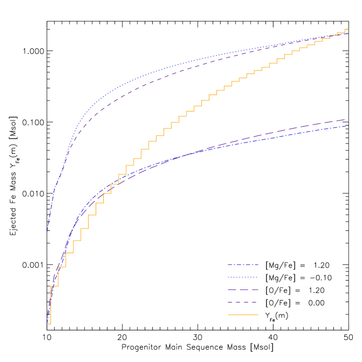
Figure 6: Iron yields $Y_{\mathrm{Fe}}\left(m\right)$ respecting the constraints given by observations of metal-poor halo stars. $Y_{\mathrm{Fe}}\left(m\right)$ starts at a very low value and increases continuously. A linear increase is not possible since the mean [el/Fe] ratios have to be conserved.

Figure 7: Distribution of [O/Fe] ratios vs. metallicity [Fe/H] of model stars resulting from the iron yields shown in Fig. 6. The slope in the distribution of the model stars is consistent with observations of oxygen abundances. A similar slope is introduced in the [Mg/Fe] distribution which can not be reconciled with observed magnesium abundances (See text for details, symbols are as in Fig. 1).

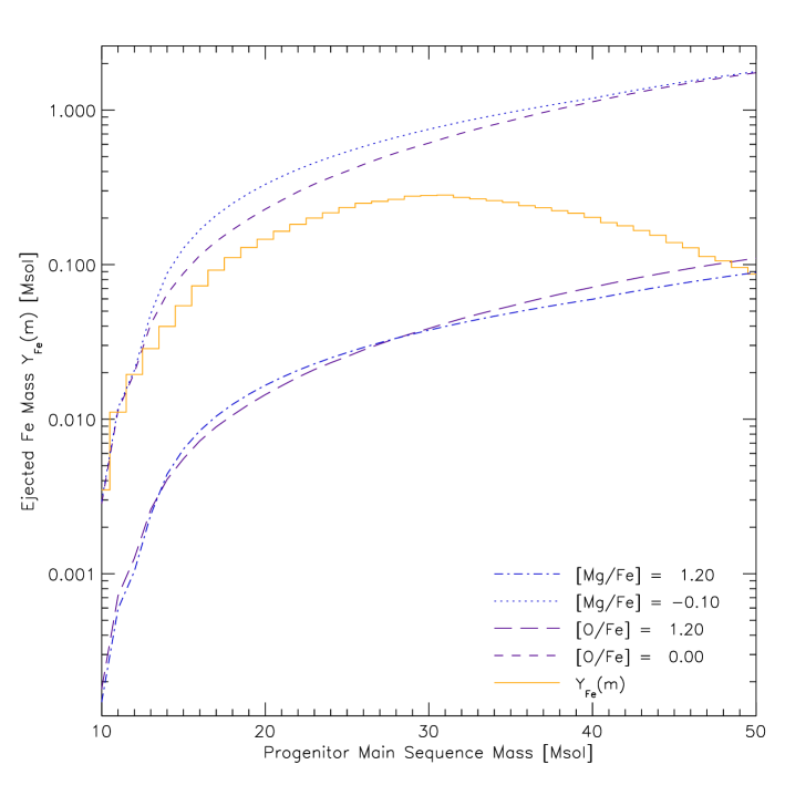
Figure 8: Iron yields $Y_{\mathrm{Fe}}\left(m\right)$ respecting the constraints given by observations of metal-poor halo stars. $Y_{\mathrm{Fe}}\left(m\right)$ starts at a somewhat higher value than in Fig. 6, reaches a maximum at about $30\,\mathrm{M}_{\sun}$ and decreases again.

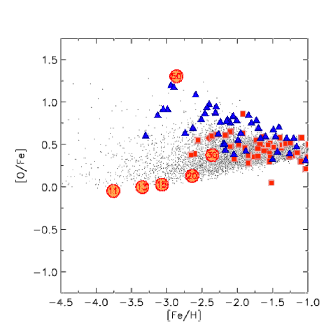
Figure 9: Distribution of [O/Fe] ratios vs. metallicity [Fe/H] of model stars resulting from the iron yields shown in Fig. 8. Clearly, the rising slope in the distribution of model stars is not consistent with observations of metal-poor halo stars. Symbols are as in Fig. 1.

Using only the constraints discussed in Sects. 4.3.1 and 4.3.2 still allows for a wide variety of possible iron yields $Y_{\mathrm{Fe}}\left(m\right)$. This is demonstrated by Figs. 6 and 8, where two simple ad hoc iron yield functions are shown. The distributions of model stars resulting from these iron yields are plotted in Figs. 7 and 9.

In Fig. 6 the iron yield $Y_{\mathrm{Fe}}\left(m\right)$ starts at the [O/Fe] $=1.2$ boundary, increases continuously with increasing progenitor mass and ends at the [O/Fe] $=0.0$ boundary. Consequently, low-mass SNe create a high [O/Fe] ratio in their surrounding primordial ISM, whereas it is close to solar in the neighbourhood of high-mass SNe. The resulting [O/Fe] distribution of model stars can be seen in Fig. 7. The distribution shows a clear trend from high to low [O/Fe] ratios with increasing [Fe/H]. A simple least-square fit to our data yields [O/Fe] $=-0.21\times[\mathrm{Fe/H}]+0.01$. This is in surprisingly good agreement with the result of King (ki00 (2000)), who finds the relation [O/Fe] $=-0.18\times[\mathrm{Fe/H}]+0.02$ after considering the effects of NLTE corrections to oxygen abundance determinations from UV OH-lines.

The reason for the slope in our model is given by the distribution of [O/Fe] and [Fe/H] ratios induced in the metal-poor ISM by core-collapse SNe with different progenitor masses, as indicated by the position of the circles in Fig. 7. All the low mass SNe with progenitors up to $15\,\mathrm{M}_{\sun}$ induce high [O/Fe] and low [Fe/H] ratios in the neighbouring primordial ISM, whereas high-mass SNe produce low [O/Fe] and high [Fe/H] ratios (recall that a constant mixing mass of $5\times 10^{4}\,\mathrm{M}_{\sun}$ per SN event is assumed, c.f. Sect. 2). SNe with intermediate masses induce [O/Fe] ratios that lie approximately on a straight line connecting the two extrema. The distribution of model stars of the first few stellar generations follows this line closely. As the mixing and chemical enrichment of the halo ISM proceeds, the distribution then converges to the IMF averaged [O/Fe] ratio. Although the inhomogeneous enrichment is responsible for the slope which is in good agreement with observations by e.g. Israelian et al. (is98 (1998)), Boesgaard et al. (bo99 (1999)), and King (ki00 (2000)), it fails to reproduce the scatter seen in observed oxygen abundances. Model stars with [O/Fe] $\approx 1.2$ exist only at [Fe/H] $\leq-3.5$ and not at [Fe/H] $\approx-2.5$, where several are observed. Furthermore, a similar slope is introduced in the [Mg/Fe] distribution ([Mg/Fe] $=-0.26\times[\mathrm{Fe/H}]-0.07$), where none is seen in observations and several model stars show [Mg/Fe] ratios as large as $\approx 1.5$. Therefore, this $Y_{\mathrm{Fe}}\left(m\right)$ has to be rejected (see however Rebolo et al. re02 (2002) concerning [Mg/Fe]).

The situation displayed in Figs. 8 and 9 is even worse. Here, the iron yield starts at the [O/Fe] $=0.0$ boundary, increases with progenitor mass, reaches its maximum around $30\,\mathrm{M}_{\sun}$, decreases again and ends at the [O/Fe] $=1.2$ boundary. The resulting distribution in [O/Fe] shows a rising slope, which is clearly in contradiction with observations. The slope is a consequence of the fact that the iron yields $Y_{\mathrm{Fe}}\left(m\right)$ of SNe in the range $10-15\,\mathrm{M}_{\sun}$ stay very close to the boundary that represents the ratio [O/Fe] $=0.0$. SNe in this mass range form the bulk of SN II events and it is therefore not surprising that their large number introduces such a slope in the distribution of model stars. Thus, this $Y_{\mathrm{Fe}}\left(m\right)$ also has to be discarded.

These simple examples show that $Y_{\mathrm{Fe}}\left(m\right)$ should not run parallel to the boundaries over a large progenitor mass interval, otherwise an unrealistic slope is introduced in the [el/Fe] distribution of model stars. They demonstrate further, that the information drawn from metal-poor halo stars alone is not sufficient to derive reliable iron yields, and that information from SN II events and the shape of the [el/Fe] distribution as function of [Fe/H] (i.e. how fast the scatter decreases and whether slopes are present or not) has to be included in our analysis.

5 Implications for stellar Fe yields

In Sect. (4.3.4) we have shown that the iron yields of lower-mass SNe (in the range $10-20\,\mathrm{M}_{\sun}$) are crucial to the distribution of model stars in [el/Fe] vs. [Fe/H] plots, since progenitors in this mass range compose the bulk (approximately 69%) of SN II events. Thus, the iron yields of lower-mass SNe should not introduce a slope in the [el/Fe] distribution but should cover the entire range of observed [O/Fe] and [Mg/Fe] ratios in order to reproduce the observations. To accomplish this, $Y_{\mathrm{Fe}}\left(m\right)$ should not lie too close to the boundaries given in Eqs. (5) and (6) in this mass range but should start at the lower boundary ([O/Fe] $=1.2$) and reach the upper boundary ([O/Fe] $=0.0$) for some progenitor in the mass range $10-20\,\mathrm{M}_{\sun}$. If the observed $\@element[56]{\mathrm{Ni}}$ production of SN 1993J, 1994I and 1987A are also taken into account, the observational constraints are stringent enough to fix the iron yields of the low mass SNe apart from small variations: $Y_{\mathrm{Fe}}\left(m\right)$ starts at the lower boundary, increases steeply in the range $10-15\,\mathrm{M}_{\sun}$ to the values given by SN 1993J and 1994I and remains almost constant in the range $15-20\,\mathrm{M}_{\sun}$ (to account for SN 1987A). For the remaining discussion we therefore assume the Fe yields in this range to be $\approx 1.5\cdot 10^{-4}\,\mathrm{M}_{\sun}$ for a $10\,\mathrm{M}_{\sun}$ progenitor, $\approx 5.5\cdot 10^{-2}\,\mathrm{M}_{\sun}$ for a $15\,\mathrm{M}_{\sun}$ progenitor and $\approx 7.0\cdot 10^{-2}\,\mathrm{M}_{\sun}$ for a $20\,\mathrm{M}_{\sun}$ progenitor. (The detailed yields resulting from our analysis are listed in Table 2). We now take a look at possible iron yields of higher mass SNe corresponding to the different models of the progenitor masses of SN 1997D and 1998bw. There are four possible combinations of the progenitor masses of those two SNe.

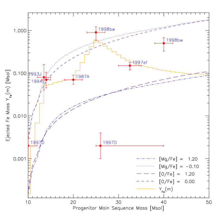
Figure 10: Model S1: Iron yields $Y_{\mathrm{Fe}}\left(m\right)$ respecting the constraints deduced from metal-poor halo stars and SN observations. The $10\,\mathrm{M}_{\sun}$ model of SN 1997D and $25\,\mathrm{M}_{\sun}$ model of SN 1998bw are assumed to be correct.

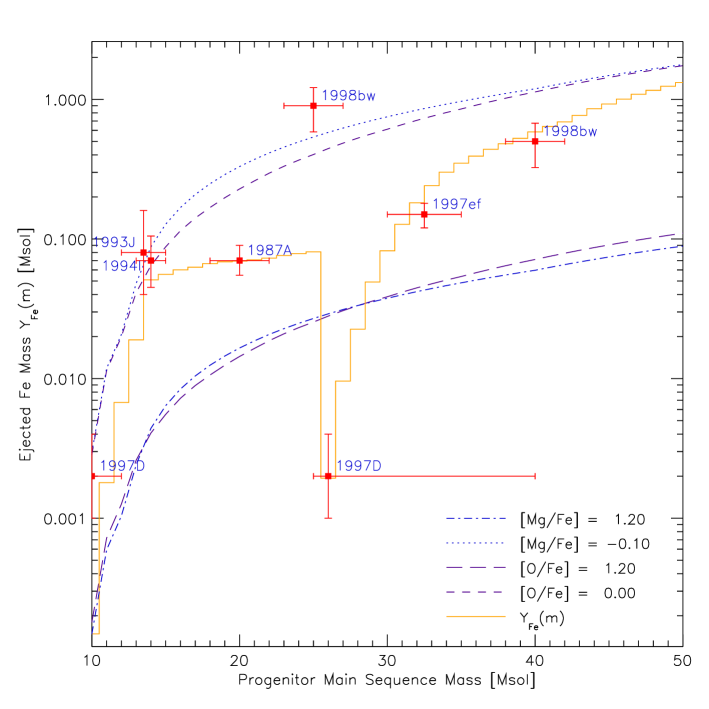
Figure 11: Model H1: Iron yields $Y_{\mathrm{Fe}}\left(m\right)$ respecting the constraints deduced from metal-poor halo stars and SN observations. The $26\,\mathrm{M}_{\sun}$ model of SN 1997D and $40\,\mathrm{M}_{\sun}$ model of SN 1998bw are assumed to be correct.

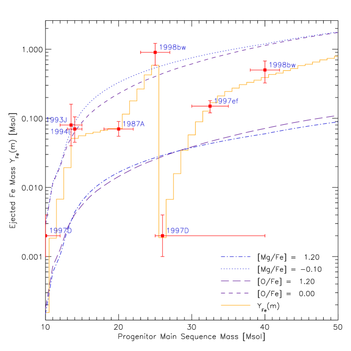
Figure 12: Model H2: Iron yields $Y_{\mathrm{Fe}}\left(m\right)$ respecting the constraints deduced from metal-poor halo stars and SN observations. The $26\,\mathrm{M}_{\sun}$ model of SN 1997D and $25\,\mathrm{M}_{\sun}$ model of SN 1998bw are assumed to be correct.

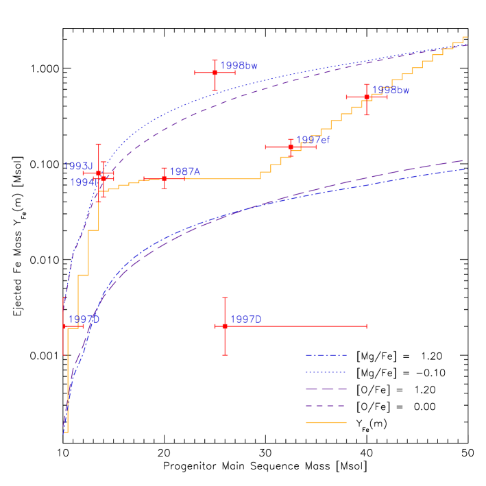
Figure 13: Model S2: Iron yields $Y_{\mathrm{Fe}}\left(m\right)$ respecting the constraints deduced from metal-poor halo stars and SN observations. The $10\,\mathrm{M}_{\sun}$ model of SN 1997D and $40\,\mathrm{M}_{\sun}$ model of SN 1998bw are assumed to be correct.

Table 2: Iron yields $Y_{\mathrm{Fe}}\left(m\right)$ proposed in Sect. 5. The first column gives the progenitor mass $m$ in solar masses. The following columns give the iron mass (in solar masses) synthesized in the corresponding SN event according to nucleosynthesis calculations of Thielemann et al. (th96 (1996)) and Nomoto et al. (no97 (1997)) – denoted by TN – and the models S1, S2, H1 and H2.

$m$	TN	S1	S2	H1	H2
10	1.6E-02	1.5E-04	1.6E-04	1.5E-04	1.5E-04
11	8.0E-02	1.9E-03	1.9E-03	1.8E-03	1.8E-03
12	1.3E-01	6.8E-03	6.8E-03	6.7E-03	6.8E-03
13	1.6E-01	2.0E-02	2.0E-02	1.9E-02	1.9E-02
14	1.6E-01	5.2E-02	5.2E-02	5.1E-02	5.1E-02
15	1.4E-01	5.5E-02	5.5E-02	5.6E-02	5.6E-02
16	1.2E-01	6.0E-02	6.0E-02	6.0E-02	6.0E-02
17	1.1E-01	6.3E-02	6.3E-02	6.3E-02	6.3E-02
18	1.0E-01	6.7E-02	6.7E-02	6.7E-02	6.7E-02
19	9.0E-02	7.0E-02	6.9E-02	6.9E-02	7.1E-02
20	8.0E-02	7.1E-02	7.0E-02	6.9E-02	7.1E-02
21	7.4E-02	1.1E-01	7.0E-02	7.1E-02	1.1E-01
22	7.0E-02	1.8E-01	7.0E-02	7.3E-02	1.8E-01
23	6.5E-02	2.7E-01	7.0E-02	7.6E-02	2.7E-01
24	6.1E-02	4.2E-01	7.0E-02	7.8E-02	4.2E-01
25	5.8E-02	5.9E-01	7.0E-02	8.1E-02	5.9E-01
26	5.9E-02	5.1E-01	7.0E-02	1.9E-03	1.9E-03
27	6.1E-02	4.3E-01	7.0E-02	9.6E-03	6.7E-03
28	6.3E-02	3.7E-01	7.0E-02	2.3E-02	1.6E-02
29	6.5E-02	3.2E-01	7.0E-02	4.9E-02	3.4E-02
30	6.7E-02	2.7E-01	8.2E-02	8.2E-02	5.8E-02
31	6.9E-02	2.2E-01	9.8E-02	1.3E-01	8.9E-02
32	7.1E-02	2.0E-01	1.2E-01	1.8E-01	1.3E-01
33	7.3E-02	1.8E-01	1.4E-01	2.4E-01	1.7E-01
34	7.5E-02	1.6E-01	1.7E-01	3.0E-01	2.1E-01
35	7.7E-02	1.5E-01	2.0E-01	3.5E-01	2.4E-01
36	7.9E-02	1.4E-01	2.3E-01	3.9E-01	2.7E-01
37	8.1E-02	1.3E-01	2.8E-01	4.4E-01	3.1E-01
38	8.3E-02	1.3E-01	3.3E-01	4.8E-01	3.3E-01
39	8.5E-02	1.2E-01	3.9E-01	5.3E-01	3.6E-01
40	8.6E-02	1.2E-01	4.6E-01	5.8E-01	3.9E-01
41	8.7E-02	1.1E-01	5.3E-01	6.4E-01	4.3E-01
42	8.7E-02	1.1E-01	6.3E-01	6.9E-01	4.5E-01
43	8.7E-02	1.0E-01	7.6E-01	7.7E-01	4.9E-01
44	8.7E-02	1.0E-01	8.8E-01	8.6E-01	5.3E-01
45	8.7E-02	9.8E-02	1.0E-00	9.3E-01	5.8E-01
46	8.7E-02	9.6E-02	1.2E-00	1.0E-00	6.1E-01
47	8.7E-02	9.6E-02	1.4E-00	1.1E-00	6.5E-01
48	8.7E-02	9.5E-02	1.6E-00	1.2E-00	7.0E-01
49	8.6E-02	9.5E-02	1.8E-00	1.2E-00	7.4E-01
50	8.6E-02	9.5E-02	2.1E-00	1.3E-00	7.9E-01

S1: The first case (model S1, shown in Fig. 10) gives the best fit to abundance observations of metal-poor halo stars. Here, we preferred the lower mass progenitor models of SN1997D and SN 1998bw over the higher mass models. The curve is characterized by a peak of $0.59\,\mathrm{M}_{\sun}$ of iron at $25\,\mathrm{M}_{\sun}$ and a slow decline of the yields down to $9.5\cdot 10^{-2}\,\mathrm{M}_{\sun}$ for the $50\,\mathrm{M}_{\sun}$ progenitor. The yields have to decline again to meet the mean abundances observed in metal-poor halo stars. Obviously, $Y_{\mathrm{Fe}}\left(m\right)$ fulfils the constraints discussed in Sects. (4.3.1), (4.3.2) and (4.3.3). Since no slope is visible in the resulting distribution of [O/Fe], [Mg/Fe], [Si/Fe] and [Ca/Fe] ratios (shown in Fig. 14), the constraint described in Sect. (4.3.4) is also respected. The distribution of model stars in [O/Fe], [Mg/Fe] and [Si/Fe] is in good agreement with the distribution of observed stars, whereas a few stars with too low [Ca/Fe] ratios are predicted. However, this may be due to the fact that Ca stems from explosive O and Si burning and therefore depend on the structure of the progenitor model and the (assumed) explosion energy (Paper I). Note, that the mean [Mg/Fe] and [Ca/Fe] ratios in the [el/Fe] plots are slightly shifted compared to the mean of observations. This problem also occurs when the original yields of TH96 are used (Paper I) and will persist for every $Y_{\mathrm{Fe}}\left(m\right)$ we present, since we did not change the mean iron yield of $0.095\,\mathrm{M}_{\sun}$ (Eq. (4)). Especially noteworthy is the good agreement in [Si/Fe], since we did not include Si in the derivation of the constraints discussed above. Moreover, the hypothetical iron yields in the other models below all result in [Si/Fe] distributions that do not fit the observations as well as model S1. Therefore, we feel that model S1 gives the best fit to element abundances in metal-poor halo stars.

H1: Fig. 11 shows the iron yields under the assumption that the higher mass models of SN 1997D and SN 1998bw are correct (model H1). Here $Y_{\mathrm{Fe}}\left(m\right)$ stays almost constant up to $25\,\mathrm{M}_{\sun}$, followed by a sudden plunge of the yields down to $1.9\cdot 10^{-3}\,\mathrm{M}_{\sun}$ to account for SN 1997D and then a continuous rise to $0.79\,\mathrm{M}_{\sun}$ of synthesized iron for the $50\,\mathrm{M}_{\sun}$ progenitor that is necessary to account for the IMF averaged yield. This sudden decrease of the iron yields could indicate a change in the explosion mechanism from supernovae with “canonical” kinetic explosion energies of $10^{51}$ erg to hypernovae with $10-100$ times higher explosion energies. However, as visible in Fig. 11, the very low iron yield of the $26\,\mathrm{M}_{\sun}$ progenitor violates the [O/Fe] $=1.2$ and [Mg/Fe] $=1.2$ boundaries derived from observations, so we would expect model stars with much too high [O/Fe] and [Mg/Fe] ratios. This is indeed the case, as can be seen in the corresponding [el/Fe] distribution (Fig. 15). A closer examination of the [el/Fe] distributions, on the other hand, reveals that these model stars are mainly present at very low metallicities ([Fe/H] $\leq-2.5$). This makes it difficult to decide, whether model H1 with its dip in $Y_{\mathrm{Fe}}\left(m\right)$ has to be discarded or not. The situation for oxygen remains unclear since no oxygen abundances were measured at metallicities where the effect is most pronounced ([Fe/H] $\leq-3.0$). However, in the range $-3.0\leq$ [Fe/H] $\leq-1.5$ there are many observations with [O/Fe] $\geq 0.6$ whereas the bulk of model stars in this range shows [O/Fe] $\approx 0.4$. Furthermore, many observations of Mg abundances in halo stars with [Fe/H] $\leq-3.0$ exist, but only one shows a ratio of [Mg/Fe] $\geq 1.0$. The remaining stars all have [Mg/Fe] $\leq 0.8$, which is in contrast to the predictions of the model. Contrary to O and Mg, there are indeed several observations of metal-poor halo stars with very high [Si/Fe] and [Ca/Fe] ratios at [Fe/H] $\leq-2.5$ and the fit in [Si/Fe] and [Ca/Fe] is not too bad. However, there are some observed stars with [Si/Fe] $\leq 0.0$ that are not reproduced by the inhomogeneous chemical evolution model. All told, model H1 clearly does not fit the observations as well as model S1.

H2: The iron yields shown in Fig. 12 (model H2) are a result of the assumption that the $26\,\mathrm{M}_{\sun}$ model of SN 1997D together with the $25\,\mathrm{M}_{\sun}$ model of SN 1998bw are correct. Coincidentally, $Y_{\mathrm{Fe}}\left(m\right)$ is also compatible with the $10\,\mathrm{M}_{\sun}$ and $40\,\mathrm{M}_{\sun}$ models of SN 1997D and SN 1998bw due to the requirement to keep the average iron yield constant. Fig. 16 shows the resulting [el/Fe] distributions. Due to the low amount of $\@element[56]{\mathrm{Ni}}$ ejected by the $26\,\mathrm{M}_{\sun}$ progenitor that is the same for models H1 and H2 (c.f. Figs. 11, 12 and Table 2), the problems in [O/Fe] and [Mg/Fe] described in the discussion of model H1 still persist. Compared to model H1, the fit in [Si/Fe] is now significantly improved, whereas model stars with [Ca/Fe] abundances that are too low are again generated by the inhomogeneous chemical evolution code (compare with model S1). However, although models H1 and H2 predict metal-poor halo stars with [O/Fe] and [Mg/Fe] ratios as high as $\approx 1.5$, they can not be clearly discarded and the discovery of stars with metallicities [Fe/H] $\leq-2.5$ and $0.8\leq$ [Mg/Fe] $\leq 1.5$ would be a strong argument for the validity of the sudden decrease in the iron yields proposed by the models H1 and H2.

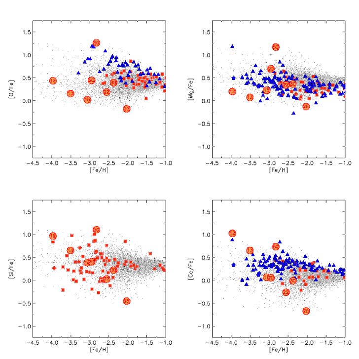
Figure 14: [el/Fe] distribution of model stars for O, Mg, Si and Ca resulting from the iron yields shown in Fig. 10 (model S1).

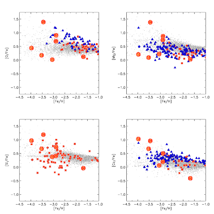
Figure 15: [el/Fe] distribution of model stars for O, Mg, Si and Ca resulting from the iron yields shown in Fig. 11 (model H1).

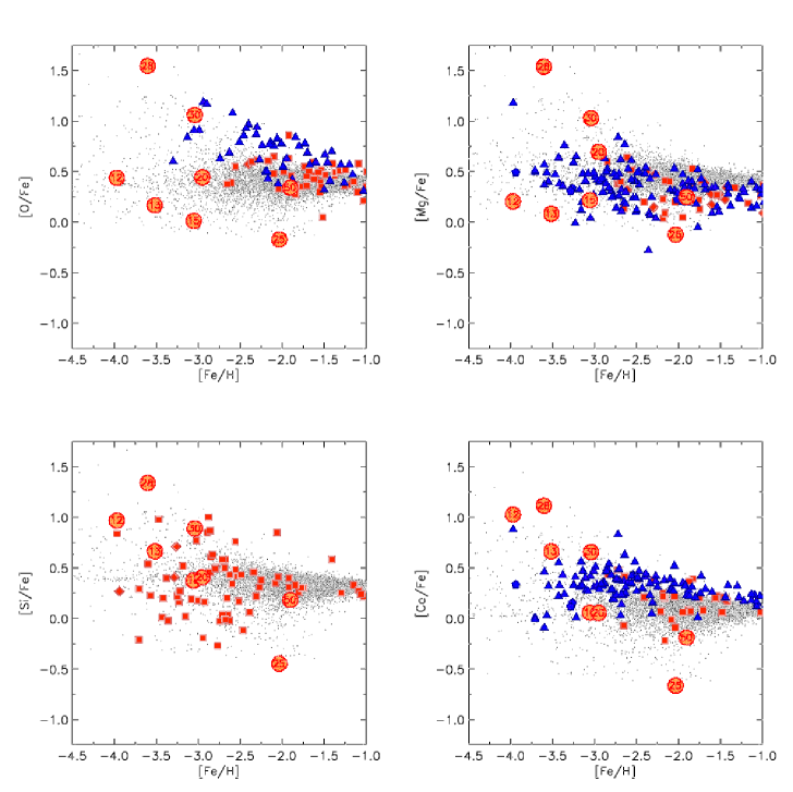
Figure 16: [el/Fe] distribution of model stars for O, Mg, Si and Ca resulting from the iron yields shown in Fig. 12 (model H2).

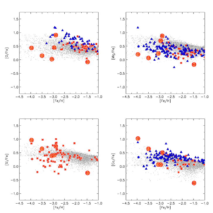
Figure 17: [el/Fe] distribution of model stars for O, Mg, Si and Ca resulting from the iron yields shown in Fig. 13 (model S2).

S2: Finally, in Fig. 13 we show possible iron yields assuming that the $10\,\mathrm{M}_{\sun}$ model of SN 1997D and $40\,\mathrm{M}_{\sun}$ model of SN 1998bw are correct (model S2). Here, $Y_{\mathrm{Fe}}\left(m\right)$ shows a plateau in the progenitor mass range from $15\,\mathrm{M}_{\sun}$ to $30\,\mathrm{M}_{\sun}$, followed by an increasing yield with increasing progenitor mass. The resulting [el/Fe] distributions are shown in Fig. 17. A shallow slope in the [el/Fe] ratios is visible in every element, violating the constraint discussed in Sect. (4.3.4). Furthermore, the scatter in [O/Fe] and [Si/Fe] clearly is not fitted by the model stars. This is especially conspicuous in the case of Si: According to the model we would expect the bulk of [Si/Fe] abundances to lie in the range $0.4\leq$ [Si/Fe] $\leq 0.8$. To the contrary, most of the observed stars have [Si/Fe] $\leq 0.4$. Model S2 therefore gives the worst fit to element abundance determinations in metal-poor halo stars.

A physical explanation for a sudden drop of the iron yields of SNe with progenitor masses around $25\,\mathrm{M}_{\sun}$ was suggested by Iwamoto et al. (iw00 (2000)): Observational and theoretical evidence indicate that stars with main-sequence masses $\mathrm{M_{ms}}\leq 25\,\mathrm{M}_{\sun}$ form neutron stars with a typical iron yield of $\approx 0.07\,\mathrm{M}_{\sun}$, while progenitors more massive than this limit might form black holes and, due to the deep gravitational potential, have a very low (or no) iron yield. This might have been the case for SN 1997D. One of the two possible models reconstructing its light-curve assumes a $26\,\mathrm{M}_{\sun}$ progenitor and a very low kinetic energy of only a few times $10^{50}$ erg and an equally low $\@element[56]{\mathrm{Ni}}$ yield of $\approx 0.002\,\mathrm{M}_{\sun}$. (But note that the lower-mass progenitor model seems more likely, c.f. Sect. 4.3.3). On the other hand, hypernovae such as 1997ef or 1998bw with progenitor masses around $30\,\mathrm{M}_{\sun}$ and $40\,\mathrm{M}_{\sun}$ and explosion energies as high as $10-100\,\times\,10^{51}$ erg might be energetic enough to allow for high iron yields even when a black hole forms during the SN event (see e.g. MacFadyen et al. mf01 (2001)). However, one of the models of SN 1998bw proposes a $25\,\mathrm{M}_{\sun}$ progenitor with a kinetic energy typical for hypernovae (i.e. much larger than the explosion energy of SN 1997D). This is in some sense a contradiction to the case of SN 1997D if we assume that a black hole formed in both cases: If the explosion mechanism is the same for SN 1998bw and SN 1997D it is natural to assume that the explosion energy scales with the mass of the progenitor and it is hard to imagine a mechanism that would account for a hypernova from a $25\,\mathrm{M}_{\sun}$ progenitor with an explosion energy that is $\approx 100$ times larger than the explosion energy from a $26\,\mathrm{M}_{\sun}$ progenitor.

Therefore, model H1 would fit nicely into the (qualitative) hypernova scenario proposed by Iwamoto et al. (iw00 (2000)), whereas models S1, S2 and H2 (yet) lack a physical explanation. On the other hand, model S1 gives a much better fit to the observations than H1, H2 and S2. Models H1 and H2 could be tested, since they predict a number of stars with very high [O/Fe], [Mg/Fe], [Si/Fe] and [Ca/Fe] ratios (up to 1.5 dex) at metallicities [Fe/H] $<-2.5$. The discovery of such ultra $\alpha$-element enhanced stars would be a strong argument in favour of the hypernova scenario proposed by Iwamoto et al. (iw00 (2000)) and the existence of a sudden drop in the iron yields of supernovae/hypernovae with progenitors around $25\,\mathrm{M}_{\sun}$.

Table 2 lists the numerical values of $Y_{\mathrm{Fe}}\left(m\right)$ as function of progenitor mass $m$ for the models discussed above. Model S1 gives the best fit to the distribution of $\alpha$-element abundances in metal-poor halo stars while S2 gives the worst. Although the models H1 and H2 violate the constraints discussed in Sect. (4.3.2) and thus do not give a fit as good as the one of S1, they cannot be ruled out on the basis of the observational data available to date.

6 Conclusions

Inhomogeneous chemical evolution models in conjunction with a current set of theoretical nucleosynthesis yields predict the existence of very metal poor stars with subsolar [O/Fe] and [Mg/Fe] ratios (Argast et al. ar00 (2000)). This result is a direct consequence of the progenitor mass dependence of stellar yields, since core-collapse SNe of different masses imprint their unique element abundance patterns on the surrounding ISM. No observational evidence of the existence of such stars is found, and recent investigations on the contrary indicate an increasing [O/Fe] ratio with decreasing metallicity [Fe/H]. This result of the inhomogeneous chemical evolution calculations is primarily due to the input stellar yields and not due to the details of the model itself. This is a strong indication that the progenitor mass dependence of existing nucleosynthesis models is not fully understood. This in itself is not surprising, since no self-consistent models of the core-collapse and the ensuing explosion exist to date (c.f. Liebendörfer et al. li01 (2001); Mezzacappa et al. me01 (2001); Rampp & Janka ra00 (2000)). A crucial parameter of explosive nucleosynthesis models is the mass-cut, i.e. the dividing line between proto-neutron star and ejecta. This gives rise to a large uncertainty in the amount of iron that is expelled in the explosion of a massive star. On the other hand, oxygen and magnesium are mainly produced during hydrostatic burning and are therefore not strongly affected by the details of the explosion mechanism. However, the distribution of [O/Mg] ratios of metal-poor halo stars suggests that either uncertainties exist even for O and Mg yields, or that observations overestimate oxygen or underestimate magnesium abundances in such metal-poor stars.

The predictions of our inhomogeneous chemical evolution model can be rectified under the assumption that the stellar yields of oxygen and magnesium reflect the true production in massive stars well enough, and by replacing the stellar iron yields of Thielemann et al. (th96 (1996)) and Nomoto et al. (no97 (1997)) by ad hoc iron yields $Y_{\mathrm{Fe}}\left(m\right)$ as function of progenitor mass $m$. These are derived in this paper from observations of metal-poor halo stars and core-collapse SNe with known progenitor and ejected $\@element[56]{\mathrm{Ni}}$ mass (the main source of $\@element[56]{\mathrm{Fe}}$ by the decay $\@element[56]{\mathrm{Ni}}$ $\rightarrow$ $\@element[56]{\mathrm{Co}}$ $\rightarrow$ $\@element[56]{\mathrm{Fe}}$). Such ad hoc iron yields have to satisfy the following constraints: First, the IMF averaged stellar yields should reproduce the mean [O/Fe] and [Mg/Fe] abundances of metal-poor halo stars. Second, the range and scatter observed in [O/Fe] and [Mg/Fe] ratios of metal-poor halo stars must be reproduced. This, in conjunction with stellar oxygen and magnesium yields, leads in turn to upper and lower boundaries for $Y_{\mathrm{Fe}}\left(m\right)$. Third, no slope should be introduced by $Y_{\mathrm{Fe}}\left(m\right)$ in the [el/Fe] distribution of model stars that is not compatible with observations. And finally, the progenitor mass dependence of the iron yields should be consistent with the ejected $\@element[56]{\mathrm{Ni}}$ mass of observed core-collapse SNe with known main-sequence mass. Here, the situation is complicated by SN 1997D and SN 1998bw. The models recovering their light-curves give in each case two significantly different progenitor masses. These constraints severely curtail the possible iron yield distributions but are not stringent enough to determine $Y_{\mathrm{Fe}}\left(m\right)$ unambiguously.

The main results of this paper are summarized in the following points:

1. Observations of O and Mg abundances in metal-poor halo stars and of the ejected $\@element[56]{\mathrm{Ni}}$ mass in core-collapse SNe, in conjunction with oxygen and magnesium yields from nucleosynthesis calculations and inhomogeneous chemical evolution models, provide a valuable tool to constrain the amount of iron ejected in a SN event as function of the main-sequence mass of its progenitor.

2. The [el/Fe] distribution of model stars as function of metallicity [Fe/H] is sensitive to the iron yields of SNe with progenitors in the mass range $10-20\,\mathrm{M}_{\sun}$. A steep increase of $Y_{\mathrm{Fe}}\left(m\right)$ from $\approx 1.5\cdot 10^{-4}\,\mathrm{M}_{\sun}$ for a $10\,\mathrm{M}_{\sun}$ progenitor to $\approx 5.5\cdot 10^{-2}\,\mathrm{M}_{\sun}$ for a $15\,\mathrm{M}_{\sun}$ progenitor followed by a slow increase to $\approx 7.0\cdot 10^{-2}\,\mathrm{M}_{\sun}$ for a $20\,\mathrm{M}_{\sun}$ progenitor is required to give an acceptable fit to the observations of metal-poor halo stars.

3. The further trend of $Y_{\mathrm{Fe}}\left(m\right)$ in the mass range $20-50\,\mathrm{M}_{\sun}$ cannot be unambiguously determined by the available data. For this mass range we have deduced four possible iron yield distributions (models S1, S2, H1 and H2) that explore the available freedom. These correspond to the four different combinations of probable progenitor masses of SN 1997D and SN 1998bw. Iron yield distributions that differ significantly form the presented models can be excluded.

4. Model S1 gives the best fit to observations while models H1 and H2 can not be ruled out. Model S2 gives the worst fit to observed [el/Fe] ratios in metal-poor halo stars. A change in the explosion mechanism of SNe II around $25\,\mathrm{M}_{\sun}$ is expected in the case of the “H” models. A test to distinguish between models S1 and H1/H2 would be the discovery of very metal-poor stars ([Fe/H] $\leq-2.5$) that are highly enriched in $\alpha$-elements.

5. Iron yield distributions derived from observations through inhomogeneous chemical evolution models yield constraints on the mass-cut in a SN II event if the detailed structure of the progenitor model is known (i.e. the size of the iron core and the zone that undergoes explosive Si burning). Thus, they can be used as benchmarks for future core-collapse supernova/hypernova models.

In future, a large and above all homogeneously analyzed sample of O, Mg and Fe abundances in very metal-poor stars is needed to derive more stringent constraints on $Y_{\mathrm{Fe}}\left(m\right)$. Not only would this allow us to determine the exact extent of the scatter in [O/Fe] and [Mg/Fe] ratios, but would also answer the important question whether the scatter in [O/Mg] is real or due to some (yet) unknown systematic errors in O and Mg abundance determinations. If the scatter in [O/Mg] turns out to be real, updated nucleosynthesis calculations including rotation and mass loss due to stellar winds are needed to understand O and Mg abundances in metal-poor halo stars.

Also very valuable would be the observation and analysis of further core-collapse supernovae/hypernovae. Only six core-collapse SNe with known progenitor and ejected $\@element[56]{\mathrm{Ni}}$ mass are known to date, and for two of them their progenitor masses are not clearly determined. Especially the discovery of a SN II with a progenitor in the critical mass range from $20-30\,\textrm{M}_{\sun}$ could provide us with the information needed to discern between the four models presented above, or at least whether the “S” or “H” models have to be preferred. This would also be a step towards answering the question whether a change in the explosion mechanism of core-collapse SNe occurs, i.e. the formation of a black hole and significant increase of the explosion energy for $m\geq 25\,\mathrm{M}_{\sun}$.

- (1) Anders, E., & Grevesse, N. 1989, Geochimica et Cosmochimica Acta, 53, 197
- (2) Argast, D., Samland, M., Gerhard, O. E., & Thielemann, F.-K. 2000, A&A, 356, 873 (Paper I)
- (3) Balachandran, S. C., & Carney, B. W. 1996, AJ, 111, 946
- (4) Bekki, K., & Chiba, M. 2000, ApJ, 534, L89
- (5) Bessel, M. S., Sutherland, R. S., & Ruan, K. 1991, ApJ, 383, L71
- (6) Beveridge, R. C., & Sneden, C. 1994, AJ, 108, 285
- (7) Boesgaard, A. M., King, J. R., Deliyannis, C. P., & Vogt, S. S. 1999, AJ, 117, 492
- (8) Bouchet, P., Danziger, I. J., & Lucy, L. B. 1991, AJ, 102, 1135
- (9) Bouchet, P., Phillips, M. M., Suntzeff, N. B., et al. 1991, A&A, 245, 490
- (10) Bouchet, P., & Danziger, I. J. 1993, A&A, 273, 451
- (11) Carretta, E., Gratton, R. G., & Sneden, C. 2000, A&A, 356, 238
- (12) Cayrel, R., Hill, V., Beers, T. C., et al. 2001, Nature, 409, 691
- (13) Chiba, M., & Beers, T. C. 2000, AJ, 119, 2843
- (14) Chugai, N. N., & Utrobin, V. P. 2000, A&A, 354, 557
- (15) Eggen, O. J., Lynden-Bell, D., & Sandage, A. R. 1962, ApJ, 136, 748
- (16) Fryer, L. C., Colgate, S. A., & Pinto, P. A. 1999, ApJ, 511, 885
- (17) Fuhrmann, K., Axer, M., & Gehren, T. 1995, A&A, 301, 492
- (18) Galama, T. J., Vreeswijk, P. M., van Paradijs, J., et al. 1998, Nature, 395, 670
- (19) Gnedin, N. Y. 1996, ApJ, 456, 1
- (20) Heger, A., Langer, N., & Woosley, S. E. 2000, ApJ, 528, 368
- (21) Heger, A. & Langer, N. 2000, ApJ, 544, 1016
- (22) Heger, A. & Woosley, S. E. 2001, astro-ph/0107037
- (23) Houck, J. C., & Fransson, C. 1996, ApJ, 456, 811
- (24) Imbriani, G., Limongi, M., Gialanella, L., et al. 2001, ApJ, 558, 903
- (25) Israelian, G., García López, R. J., & Rebolo, R. 1998, ApJ, 507, 805
- (26) Israelian, G., Rebolo, R., García López, R. J., et al. 2001, ApJ, 551, 833
- (27) Idiart, T., & Thévenin, F. 2000, ApJ, 541, 207
- (28) Iwamoto, K., Nomoto, K., Höflich, P., et al. 1994, ApJ 437, L115
- (29) Iwamoto, K., Mazzali, P.A., Nomoto, K., et al. 1998, Nature 395, 672
- (30) Iwamoto, K. 1999a, ApJ, 512, L47
- (31) Iwamoto, K. 1999b, ApJ, 517, L67
- (32) Iwamoto, K., Takayoshi, N., Nomoto, K., et al. 2000, ApJ, 534, 660
- (33) Jehin, E., Magain, P., Neuforge, C., et al. 1999, A&A, 341, 241
- (34) King, J. R. 1994, ApJ, 436, 331
- (35) King, J. R. 2000, AJ, 120, 1056
- (36) Klypin, A., Kravtsov, A. V., Valenzuela, O., & Prada F. 1999, ApJ, 522, 82
- (37) Kozma, C., & Fransson, C. 1998, ApJ, 497, 431
- (38) Liebendörfer, M., Mezzacappa, A., Thielemann, F.-K., et al. 2001, Phys. Rev. D, 6310, 3004
- (39) MacFadyen, A. I., Woosley, S. E., & Heger, A. 2001, ApJ, 550, 410
- (40) Maeder, A. 1992, A&A, 264, 105
- (41) Maeder, A. & Meynet, G. 2000, ARA&A, 38, 143
- (42) Magain, P. 1989, A&A, 209, 211
- (43) McWilliam, A., Preston, G. W., Sneden, C., & Searle, L. 1995, AJ, 109, 2757
- (44) Meynet, G. & Maeder, A. 2000, A&A, 361, 101
- (45) Mezzacappa, A., Liebendörfer, M., Messer, O. E. B., et al. 2001, Phys. Rev. Letters, 86, 1935
- (46) Molaro, P., & Bonifacio, P. 1990, A&A, 236, L5
- (47) Molaro, P., & Castelli, F. 1990, A&A, 228, 426
- (48) Moore, B., Ghigna, S., Governato, F., et al. 1999, ApJ, 524, L19
- (49) Nakamura, T., Umeda, H., Iwamoto, K., et al. 2001, ApJ, 555, 880
- (50) Navarro, J. F., & Steinmetz, M. 2000, ApJ, 538, 477
- (51) Nissen, P. E., Gustafsson, B., Edvardsson, B., & Gilmore, G. 1994, A&A, 285, 440
- (52) Nomoto, K., Hashimoto, M., Tsujimoto, T., et al. 1997, Nucl. Phys., A161, 79c13
- (53) Norris, J. E., Peterson, R. C., & Beers, T. C. 1993, ApJ, 415, 797
- (54) Pearce, F. R., Jenkins, A., Frenk, C. S., et. al. 1999, ApJ, 521, L99
- (55) Peterson, R. C., Kurucz, R. L., & Carney, B. W. 1990, ApJ, 350, 173
- (56) Primas, F., Molaro, P., & Castelli, F., 1994 A&A, 290, 885
- (57) Rampp, M., & Janka, H.-T. 2000, ApJ, 539, L33
- (58) Rauscher, T., Heger, A., Hoffman, R. D. & Woosley S. E. 2002, astro-ph/0112478
- (59) Rebolo, R., et al. 2002, in preparation
- (60) Ryan, S. G., Norris, J. E., & Bessell, M. S. 1991, AJ, 102, 303
- (61) Ryan, S. G., Norris, J. E., & Beers, T. C. 1996, ApJ, 471, 254
- (62) Samland, M. 1997, ApJ, 496, 155
- (63) Searle, L., & Zinn, R. 1978, ApJ, 225, 357
- (64) Shigeyama, T., & Nomoto, K. 1990, ApJ, 360, 242
- (65) Shigeyama, T., Suzuki, T., Kumagai, S., & Nomoto, K. 1994, ApJ, 420, 341
- (66) Shigeyama, T., & Tsujimoto, T. 1998, ApJ, 507, L135
- (67) Sneden, C., Preston, G. W., McWilliam, A., & Searle, L. 1994, ApJ, 431, L27
- (68) Sollerman, J., Kozma, C., Fransson, C., et al. 2000, ApJ, 537, L127
- (69) Spiesman, W. J., & Wallerstein, G. 1991, AJ, 102, 1790
- (70) Spite, M., & Spite, F. 1991, A&A, 252, 689
- (71) Steinmetz, M., & Müller, E. 1995, MNRAS, 276, 549
- (72) Suntzeff, N. B., & Bouchet, P. 1990, AJ, 99, 650
- (73) Suntzeff, N. B., Phillips, M. M., Elias, J. H., et al. 1992, ApJ, 384, L33
- (74) Thielemann, F.-K., Hashimoto, M., & Nomoto, K. 1990, ApJ, 349, 222
- (75) Thielemann, F.-K., Nomoto, K., & Hashimoto, M. 1996, ApJ, 460, 408 (TH96)
- (76) Thomas, D., Greggio, L. & Bender, R. 1998, MNRAS, 296, 119
- (77) Turatto, M., Mazzali, P. A., Young, T. R. et. al., 1998, ApJ 498, L129
- (78) Woosley, S. E., & Weaver, T. A. 1995, ApJS, 101, 181 (WW95)