Morphological Measures of nonGaussianity in CMB Maps

Abstract

We discuss the tests of nonGaussianity in CMB maps using morphological statistics known as Minkowski functionals. As an example we test degree-scale cosmic microwave background (CMB) anisotropy for Gaussianity by studying the QMASK map that was obtained from combining the QMAP and Saskatoon data. We compute seven morphological functions $M_{i}({\Delta T})$, $i=1,...,7$: six Minkowski functionals and the number of regions $N_{c}$ at a hundred ${\Delta T}$ levels. We also introduce a new parameterization of the morphological functions $M_{i}(A)$ in terms of the total area $A$ of the excursion set. We show that the latter considerably decorrelates the morphological statistics and makes them more robust because they are less sensitive to the measurements at extreme levels. We compare these results with those from 1000 Gaussian Monte Carlo maps with the same sky coverage, noise properties and power spectrum, and conclude that the QMASK map is neither a very typical nor a very exceptional realization of a Gaussian field. At least about 20% of the 1000 Gaussian Monte Carlo maps differ more than the QMASK map from the mean morphological parameters of the Gaussian fields.

1 Introduction

The issue of Gaussianity of CMB maps plays a crucial role in testing assumptions about the early Universe. The simplest inflation models strongly favor Gaussianity of the primordial inhomogeneities (see Turner, 1997, and references therein), whereas other scenarios assuming cosmic strings or topological defects (see Vilenkin and Shellard, 1994, and references therein) predict non-Gaussian perturbations. Gaussianity is also a key underlying assumption of all experimental power spectrum analyses to date, entering into the computation of error bars (Tegmark, 1997; Bond and Jaffe, 1998), and therefore needs to be observationally tested. A third reason for studying Gaussianity of CMB maps is that it may reveal otherwise undetected foreground contamination.

Numerous tests of Gaussianity in the COBE maps (Colley, Gott, and Park, 1996; Kogut et al., 1996; Ferreira, Magueijo, and Górski, 1998; Pando, Valls-Gabaud, and Fang, 1998; Bromley and Tegmark, 1999; Novikov, Feldman, and Shandarin, 1999; Banday, Zaroubi, and Górski, 2000; Barreiro et al., 2000; Magueijo, 2000; Mukherjee, Hobson, and Lasenby, 2000; Aghanim, Forni, and Bouchet, 2001; Phillips and Kogut, 2001) have resulted in the general agreement that all non-Gaussian signals were of noncosmological origin. This was not unexpected because of COBE’s low ($7^{\circ}$ deg) angular resolution.

Testing Gaussianity on smaller scales may bring much more interesting results. The first study of Gaussianity on degree scale showed the consistency of the QMASK map with the assumption of the Gaussianity (Park et al., 2001). However, this study tested only the Gaussianity of the topology of the map. The study of the MAXIMA-1 anisotropy data also showed the consistency with the Gaussianity in the range between 10 arc-minutes and 5 degrees (Wu et al., 2001). A total of 82 tests for Gaussianity were made in this study. Although performing many tests is always better than few it is not clear how independent these tests were.

The question of statistical independence of different non-Gaussianity tests is complicated. However, in some simple cases some of the tests can be statistically disentangled. For instance, consider the probability function, which is perhaps the simplest test for non-Gaussianity. It easy to transform the probability function to any given form simply by relabeling the contours using a monotonic function. This relabeling obviously does not have any effect on the morphology of the field since every contour line remains the same as well as the order of levels due to monotonicity of the transformation. However, this transformation may strongly affect the whole hierarchy of the $n$-point correlation functions. This is of course due to well known connection of the probability function to all $n$-point functions.

Genus represents only one statistic sensitive to non-Gaussianity. It may detect some types of non-Gaussianity and be not sensitive to the others. Consider, for instance, the following mapping of a Gaussian field $\phi(x,y)$ into $\Phi(X,Y)$

$$\Phi(X,Y)=\phi(x,y),$$ (1)

where

$$X = x+\tau u(x,y),$$

$$Y = y+\tau v(x,y).$$ (2)

Equation 1 guarantees that every level label remains unchanged, while the level lines are shifted and deformed according to eqs. 2. Functions $u(x,y)$ and $v(x,y)$ can be any smooth functions including random functions. At small $\tau$ before caustics have occurred, the mapping $(x,y)\rightarrow(X,Y)$ is single valued and therefore the contour map of $\Phi(X,Y)$ is one-to-one image of $\phi(x,y)$, although geometrically distorted. The genus of the $\Phi(X,Y)$ field as a function of the level remains exactly the same (i.e. Gaussian) as that of the $\phi(x,y)$ field because the mapping is continous and nonsingular and therfore preserves toplogy. On the other hand, the mapping $(x,y)\rightarrow(X,Y)$ can be neither isometric (conserving the lengths) nor area-preserving and therefore both the areas and the contours of the excursion sets may be distorted. As a result, the $\Phi(X,Y)$ can be a strongly non-Gausssian field having exactly the Gaussian genus in the level parameterization. Perhaps, it is worth noting that a particular case of the above example ($u(x,y)=\partial\psi(x,y)/\partial x$ and $v(x,y)=\partial\psi(x,y)/\partial y$) corresponds to viewing the Gaussin contour map $\phi(x,y)$ through a glass layer with varying thickness $\psi(x,y)$ (see e.g. Zel’dovich, Mamaev, and Shandarin (1983); Shandarin and Zel’dovich (1989)).

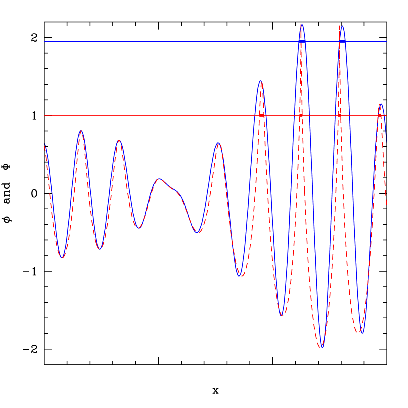
Figure 1: One-dimensional illustration of a non-Gaussian field $\Phi$ (dashed line) having exactly same number of peaks (which is analogous to genus in 2D) in the level parameterization as the Gaussian field $\phi$ (solid line). Compare the number of peaks in two fields at two levels marked by the dotted and dash-dotted horizontal lines. The length parameterization in 1D is analogous to the area parameterization in 2D. In order to compare the number of peaks in the length parameterization one has to count the peaks of the two fields at different levels. The marked levels are chosen in such a way that the total length of the excursion set of the non-Gaussian field at $\Phi=1.$ (the sum of four heavy segments) equals the total length of the the excursion set of the Gaussian field at $\phi=1.95$ (the sum of two heavy segments).

A one-dimensional illustration of the above field is shown in Fig. 1. A realization of the Gaussian field $\phi(x)$ is shown by the solid line and of the non-Gaussian field $\Phi(x)$ by the dashed line. The total area of the excursion set in 2D is analogous to the total length of the excursion set in 1D and the genus in 2D is analogous to the number of peaks in 1D. The level parameterization means the comparison of the number of peaks in the two fields at the same level. Both fields have the same number of peaks at every level as illustrated by the dotted and dash-dotted horizontal lines. However, the total lengths occupied by the peaks of the $\phi(x)$ and $\Phi(x)$ fields are different at a given level. The length parameterization in 1D means that the comparison of the numbers of peaks must be done at the same total length of the excursion sets which generally happens at different levels for the $\phi(x)$ and $\Phi(x)$ fields. For instant, the length of the excursion set of the Gaussian field at $\phi(x)=1.95$ (the sum of two heavy line segments at level $=1.95$) equals the length of the excursion set of the non-Gaussian field at $\Phi(x)=1$ (the sum of four heavy line segments at level $=1$) . One can see at this total length the number of peaks in the Gaussian field is two while in the non-Gaussian field it is four. Thus, the number of peaks parameterized by the total length does detect this type of non-Gaussianity while the number of peaks parameterized by the level does not. Similarly, the area parameterization of the genus in two dimensions does detect this type of non-Gaussianity while the level parameterization of the genus statistic does not.

If the mapping (eq. 2) is area-preserving than the genus of the $\Phi(X,Y)$ field remains exactly Gaussian also in the area parameterization. Thus, a detection of such non-Gaussianity requires additional tests.

We use two different parameterization of the measured morphological characteristics and show that the parameterization by the total area of the excursion set (i.e. the cumulative probability function) has an advantage over parameterization by the temperature because it gives considerably smaller correlations between different measures. In particular, the total area parameterization detects non-Gaussianity by the genus statistic in the above example while the temperature parameterization does not. For additional discussion of this issue, see Shandarin (2002).

Along with the QMASK map (Xu et al. 2001), we analyze a thousand reference maps with the same sky coverage, noise properties and power spectrum as the QMASK map. For each map we compute seven morphological functions at a hundred temperature/area levels. These functions are:

1. the total area of the excursion set $A({\Delta T})$,

2. the total contour length $C({\Delta T})$ and $C(A)$ ,

3. the genus of the excursion set $G({\Delta T})$ and $G(A)$ ,

4. the area of the largest (by area) region $A_{p}({\Delta T})$ and $A_{p}(A)$ ,

5. its perimeter $C_{p}({\Delta T})$ and $C_{p}(A)$,

6. genus $G_{p}({\Delta T})$ and $G_{p}(A)$, and finally

7. the number of regions $N_{c}({\Delta T})$ and $N_{c}(A)$ .

The first three are the global Minkowski functionals and the following three are the Minkowski functionals of the largest (by area) region. The largest region at some threshold spans the whole map, or “percolates”. Its Minkowski functionals are the best indicators of the percolation phase transition (Shandarin, 1983; Yess and Shandarin, 1996). Our notations reflect some of the jargon used in cluster analysis: $A_{p},C_{p},G_{p}$ for the Minkowski functionals of the percolating region and $N_{c}$ for the number of regions, often referred to as “clusters” in cluster analysis.

We then calculate the mean for each of these fourteen functions ($\bar{M_{i}}({\Delta T})$ and $\bar{M_{i}}(A),~{}i=1,\cdots,7$) computed from a thousand Gaussian maps and quantify the differences of every function for every map with respect to the mean functions in quadratic measure. Finally, we compute these differences for the QMASK map and test the Gaussianity hypothesis by comparing them to the thousand reference maps.

The rest of the paper is organized as follows. In Sec. 2 and 3 we briefly describe the QMASK map and the Gaussian simulations thereof. In Sec. 4 we define the morphological functions, their parameterization and the method of quantifying the departure from the Gaussianity. In Sec. 5 we summarize the results.

2 QMASK Map

The QMASK map, described in (Xu et al., 2001), combines all the information from the QMAP (Devlin et al., 1998; Herbig et al., 1998; de Oliveira-Costa et al., 1998) and Saskatoon (Netterfield et al., 1995, 1997; Tegmark et al., 1996) experiments into a single map at 30-40 GHz covering about 648 square degrees around the North Celestial Pole. The map consists of sky temperatures in 6495 sky pixels, conveniently grouped into a 6495-dimensional vector ${\bf x}$, with a FWHM angular resolution of $0.68^{\circ}$. As detailed in Xu et al. (2001), all the complications of the map making and deconvolution process are encoded in the corresponding $6495\times 6495$ noise covariance matrix ${\bf N}$. The map has a vanishing expectation value $\langle{\bf x}\rangle={\bf 0}$ and a covariance matrix given by

$${\bf C}\equiv\langle{\bf x}{\bf x}^{t}\rangle={\bf N}+{\bf S},$$ (3)

where the signal covariance matrix ${\bf S}$ is given by

$${\bf S}_{ij}=\sum_{\ell=2}^{\infty}{\ell(\ell+1)\over 4\pi}P_{\ell}(\widehat{\bf r}_{i}\cdot\widehat{\bf r}_{j})e^{-\theta^{2}\ell(\ell+1)}C_{\ell},$$ (4)

the $P_{\ell}$ are Legendre polynomials, $C_{\ell}$ is the angular power spectrum, $\widehat{\bf r}_{i}$ is a unit vector pointing towards the $i^{\rm th}$ pixel, and $\theta=$FWHM$/\sqrt{8\ln 2}$ is the rms beam width. When computing ${\bf S}$ in practice, we use the smooth power spectrum of (Xu, Tegmark, and de Oliveira-Costa, 2001) that fits the observed QMASK power spectrum measurements.

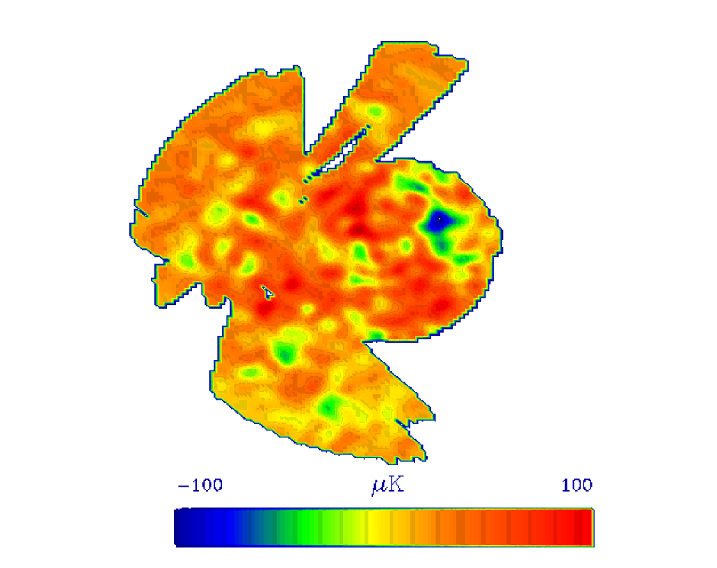
Figure 2: Grey scale QMASK map. Light color correspond to higher temperatures. Note that there are three clearly distinct white regions in the map where data are absent.

Since the raw map has a large and complicated noise component, we work with the Wiener-filtered version of the map in this paper, shown in Fig. 2 and defined as

$${\bf x}_{w}\equiv{\bf W}{\bf x},\quad{\bf W}\equiv{\bf S}({\bf N}+{\bf S})^{-1}.$$ (5)

This approach was also taken in Park et al (2001) and Wu et al (2001).

3 Mock Maps

In order to quantify the statistical properties of our Minkowski functionals, we need large numbers of simulated QMASK maps. We therefore generate one thousand mock Gaussian maps as follows. The covariance matrix ${\bf C}_{w}$ of the Wiener-filtered map is given by

$${\bf C}_{w}\equiv\langle{\bf x}_{w}x_{w}^{t}\rangle=\langle({\bf W}{\bf x})({\bf W}{\bf x})^{t}\rangle={\bf W}\langle{\bf x}{\bf x}^{t}\rangle{\bf W}^{t}={\bf W}{\bf C}{\bf W}^{t},$$ (6)

and we Cholesky-decompose it as ${\bf C}_{w}={\bf L}{\bf L}^{t}$, where the matrix ${\bf L}$ lower triangular. It is straightforward to show that if ${\bf z}$ is a vector of independent Gaussian random variables with zero mean and unit variance (which is trivial to generate numerically), i.e., $\langle{\bf z}{\bf z}^{t}\rangle={\bf I}$, the identity matrix, then the mock maps defined ${\bf x}_{m}\equiv{\bf L}{\bf z}$ will have a multivariate Gaussian distribution with $\langle{\bf x}_{m}{\bf x}_{m}^{t}\rangle={\bf C}_{w}$.

4 Morphological Statistics

In this paper we use a set of morphological statistics based on Minkowski functionals. As suggested by (Novikov, Feldman, and Shandarin, 1999), one can use both global and partial Minkowski functionals in studies of CMB maps. In this study we use the global Minkowski functionals and those of the largest region by area (the so-called percolating region).

4.1 Global Minkowski functionals

Global Minkowski functionals were introduced into cosmology as quantitative measures of CMB anisotropy by Gott et al. (1990) although without reference to the Minkowski functionals and thus without stressing their unique role in differential and integral geometry. Mecke, Buchert, and Wagner (1994) were the first to place the studies of morphology of the large scale structure in the context of differential and integral geometry. In particular, they emphasized a powerful theorem by (Hadwiger, 1957) stating that with rather broad restrictions, the set of Minkowski functionals provides a complete description of the morphology (for further discussion see Kerscher, 1999).

Global Minkowski functionals describe the morphology of the excursion set at a chosen threshold: $A({\Delta T})$, $C({\Delta T})$ and $G({\Delta T})$ are the total area, contour length and genus of the excursion set, respectively. The Minkowski functionals of Gaussian fields are known analytically as functions of the threshold. Assuming that the field is normalized, i.e. $u=({\Delta T}-<{\Delta T}>)/\sigma_{{\Delta T}}$ so that $<u>=0,<u^{2}>=1$, the Minkowski functionals are

$$A(u) = \frac{1}{2}\left[1-{\rm erf}\left(\frac{u}{\sqrt{2}}\right)\right],$$ (7)

$$C(u) = \frac{1}{2R}\exp\left(-\frac{u^{2}}{2}\right),$$ (8)

$$G(u) = \frac{1}{(2\pi)^{\frac{3}{2}}}\frac{1}{R^{2}}u\exp\left(-\frac{u^{2}}{2}\right),$$ (9)

where $R=\sqrt{2}/\sigma_{1}$ is the characteristic scale of fluctuations in the field; $\sigma_{1}$ is the rms of the first derivatives (in statistically isotropic fields both derivatives $\partial u/\partial x$ and $\partial u/\partial y$ have equal rms). $A(u)$ is the fraction of the area in the excursion set and thus equals the cumulative probability function: $A(u)=\int_{u}^{\infty}p(u^{\prime})du^{\prime}$, where $p(u)$ is the probability function. $C(u)$ and $G(u)$ are the length of the contour and the genus of the excursion set per unit area respectively.

In this study we use somewhat different normalization and units. We measure the total contour length in the mesh units and we define $G$ as the number of isolated regions minus the number of holes in the excursion set.

4.2 Percolating region

The morphology of every isolated region in the excursion set can be characterized by three partial Minkowski functionals : the area, boundary contour length and genus of the region. In order to describe the morphology of the field in more detail, Novikov, Feldman, and Shandarin (1999) used the distribution functions of the partial Minkowski functionals at several level thresholds. Bharadwaj et al. (2000) used the averaged shape parameters in the study of the morphology in the LCRS slices. Here we choose to utilize only the Minkowski functionals of the largest region ($A_{p}({\Delta T}),C_{p}({\Delta T}),G_{p}({\Delta T})$) in addition to the global Minkowski functionals . This is dictated by the relatively small size of the QMASK map: the maximum number of isolated regions is about 30 and therefore the distribution functions are very noisy. The Minkowski functionals of the largest, i.e. , percolating region of Gaussian fields are not known in an analytic form but can be easily measured in Monte Carlo simulations (Shandarin, 2002).

An additional comment may be useful. A naive idea of percolation invokes an image of the region connecting the oposite sides of the map. Thus, the question may arise: what does percolation mean in a map with complex boundaries and holes like the QMASK map (Fig. 2). In particular, which points must be connected at the percolation threshold in a map with irregular boundaries? The fact is that percolation is a phase transition which takes place regardless of the shape and topology of the map (see e.g. Stauffer and Aharony (1992)). It can be studied and relatively easily measured in maps of arbitrary shapes including holes. The Minkowski functionals of the largest region are particularly useful while the direct detection of the connection between the oposite sides is much more unstable even in simple square maps (Dominik and Shandarin, 1992). At percolation transition the area and perimeter of the largest region experience a rapid growth while the genus rapidly decreases (Shandarin, 2002). Similarly to many other statistics the percolation transition is affected mostly by the size of the map and its effective dimensions and much less by its shape or presence of holes. For example, if a three-dimensional map has the shape of a thin wedge then percolation becomes two-dimensional (Shandarin and Yess, 1998). Likewise, a two-dimensional map having the shape of a narrow strip effectively percolates as a one-dimensional map. More accurately, if the smallest size of the map is smaller than the scale of the field then the percolation transition effectively reduces the dimensions. A simple visual inspection of Fig. 2 shows that nothing of the kind of the problems discussed above is present in the QMASK map. The major drawback of the map is its size not the shape.

In addition, we wish to stress that we do not compare the percolation curves measured for the QMASK map with the standard Gaussian curves. Instead we compare them with the curves measured in the reference maps having exactly same irregular shape and holes as the QMASK map. Therefore, the question of accuracy of reproduction of the standard percolation properties in two-dimensional maps becomes largely irrelevant.

4.3 Numerical technique

The numerical technique used for measuring the Minkowski functionals is described in detail in (Shandarin, 2002). Here we outline the main features that may differ from numerical methods used by others (Coles, 1988; Gott et al., 1990; Schmalzing and Buchert, 1997; Winitzki and Kosowsky, 1997; Schmalzing and Górski, 1998; Park et al., 2001; Wu et al., 2001).

First, we use neither Koendernik invariants (Koenderink, 1984) nor Croftons’s formulae (Crofton, 1968) which are often used in other studies. A pixelized map is considered to be an approximation to a continuous field. This approach was used by Novikov, Feldman, and Shandarin (1999) but here we use a different and more refined version of the code computing Minkowski functionals . The major effect of this improvement is the numerical efficiency of the code.

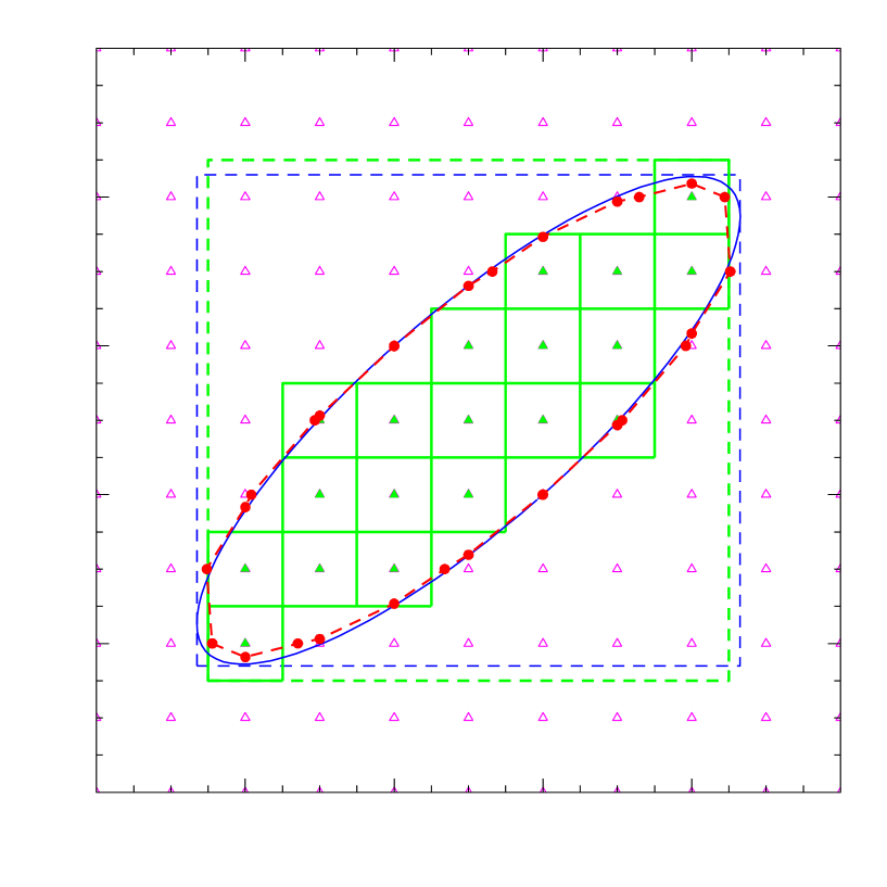
Figure 3: An illustration of the numerical technique. The solid line shows the elliptical contour corresponding to the certain threshold $u=u_{th}$. Triangles mark the sites of the lattice: solid with $u>u_{th}$ and empty with $u<u_{th}$. Solid circles mark the contour points satisfying the condition $u=u_{th}$ (the roots of eq. 10); the dashed line is the resulting contour. The true area of the region is the area within the solid ellipse. We approximate it by the area within the dashed contour while in most works it is approximated by the sum of areas of the elementary squares (solid squares). We approximate the perimeter by the length of the dashed contour while in other works it is often approximated by the sum of the external edges of the elementary squares. One can easily see that this approximation gives the value of the perimeter of the large dotted rectangle. As the lattice constant approaches zero it converges to the perimeter of the large solid rectangle, while our perimeter converges to the true value of the perimeter of the solid ellipse.

The major features of our technique are illustrated by Fig. 3. Suppose we use a regular square lattice and the true contour corresponding to $u=u_{th}$ is a simple ellipse shown by the solid line in Fig. 3. The sites satisfying the threshold condition $u>u_{th}$ are shown by filled triangles, while the sites with $u<u_{th}$ are shown by empty triangles. The union of elementary squares (shown by heavy solid lines) placed on each site satisfying the threshold condition is widely used as an approximation to the region. One can easily count the number of elementary squares, number of edges of the elementary squares and number of vertices in the union. Then by using Crofton’s formulae one computes the area, perimeter and the Euler characteristic of the region. For instance, the area in this approximation is simply the sum of areas of the elementary squares. The perimeter is the number of external edges of the elementary squares. While the area converges to the right value as the lattice constant approaches zero, the perimeter does not (for a detailed discussion of this effect see e.g. Winitzki and Kosowsky (1997)). The perimeter of the set of the elementary squares obviously equals the perimeter of the rectangular region shown by the dotted line. As the lattice parameter approaches zero the perimeter of the region approches the perimeter of the large rectangle shown by the solid line which obviously is a wrong value. Assuming the isotropy of the map one can show that the mean length of a segment is $4/\pi$ times larger than its true value (Winitzki and Kosowsky, 1997) and can be corrected only statistically. Our method is completely free of this drawback and does not need such a correction.

In our approach we begin with the construction of the contour points for each isolated region of the excursion set. Suppose that $u(i,k)<u_{th}$ but $u(i+1,k)\geq u_{th}$ then the contour point lies somewhere between ($i,k$) and ($i+1,k$) sites. Its coordinates ($x,y_{k}$) can be obtained by solving the linear interpolation equation

$$u_{th}=u(i,k)+\frac{u(i+1,k)-u(i,k)}{x(i+1,k)-x(i,k)}(x-x(i,k))$$ (10)

for the coordinate $x$. We construct the contour points by linear interpolation of the field between the sites in both horizontal and vertical directions. These points are marked by the solid circles in Fig. 3. Then, computing the perimeter we assume that the contour points are connected by the segments of a straight line (dashed line). The contours made by this method converges to the right value of the perimeter as the lattice constant approaches zero.

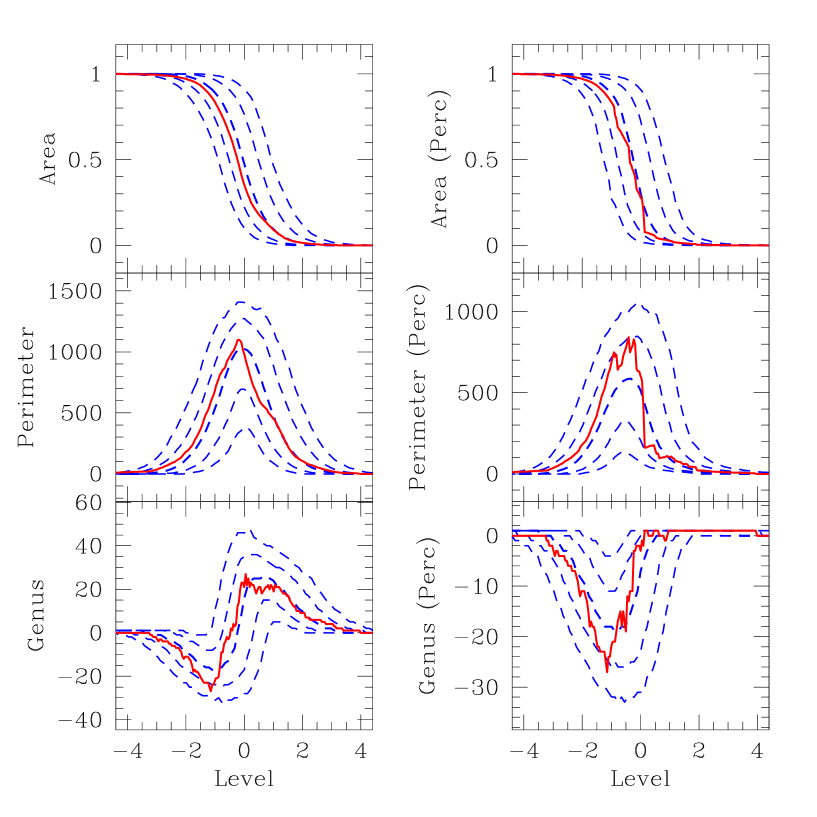
Figure 4: Minkowski functionals as functions of $u={\Delta T}/\sigma_{{\Delta T}}$ for the excursion set (left hand side column) and for the percolating region (right hand side column). Top row: the area fraction $A$ and $A_{p}$, middle row : contour length $C$ and $C_{p}$, bottom row: genus $G$ and $G_{p}$. The contour lengths are given in mesh units. The genus is “number of regions” $-$ “number of holes”. The solid lines show the parameters of the QMASK map, heavy dashed lines show the median Gaussian values, thin dashed lines show 68% and 95% ranges.

The other major difference consists in allowing a direct linkage of diagonal grid sites in some cases depending on the values in the four neighboring sites. Consder a case when two diagonally adjacent pixels satisfy the threshold condition: $u(i,k)\geq u_{th}$ and $u(i+1,k+1)\geq u_{th}$ but the sites $u(i+1,k)<u_{th}$ and $u(i,k+1)<u_{th}$. One usually chooses either consider the $(i,k)$ and $(i+1,k+1)$ sites always directly linked or always not linked implying that the difference between the two alternatives disappears with vanishing the lattice parameter. Our definition of the direct linkage of two diagonally adjacent pixels is different from both. The diagonally adjacent pixels are directly linked if $u_{mean}=(u(i,k)+u(i+1,k)+u(i,k+1)+u(i+1,k+1))/4\geq u_{th}$ and directly not linked otherwise. In the latter case they of course are allowed to be linked by the friend of friend procedure if they have proper friends. This method affects the number of regions, their sizes and the number of holes in the regions and therefore the values of all Minkowski functionals (including genus). The visual inspection of Fig. 4 and Fig. 4 in Park et al. (2001) reveals small but noticeable differences in the genus curves. This treatment of the direct diagonal linkage also considerably reduces the intrinsic anisotropy of a rectangular grid. Since the QMASK map occupies a small part of the sky, we ignore the intrinsic curvature of the map when computing the areas and perimeters.

If a part of the region boundary is the boundary of the map mask, then it does not contribute to the contour length of the region. Similarly, the holes in the map mask contribute neither into the genus nor the contour length.

The analysis of one realization of a Gaussian random field at a hundred levels takes about 0.7s, 2.9s, 12.3s, and 73s for $64^{2}$, $128^{2}$, $256^{2}$, and $512^{2}$ maps respectively on HP C240 workstation. It corresponds approximately to the $t\propto N_{pix}\ln(N_{pix})$ dependence of the computational time on the size of the map.

4.4 Parameterization by the level of ${\Delta T}$.

In addition to six Minkowski functionals , we computed the number of isolated regions $N_{c}$ (Novikov, Feldman, & Shandarin 1999). Thus, in total we compute seven morphological parameters

$$M_{i}({\Delta T})=[A({\Delta T}),C({\Delta T}),G({\Delta T}),A_{p}({\Delta T}),C_{p}({\Delta T}),G_{p}({\Delta T}),N_{c}({\Delta T})],~{}~{}~{}i=1,...,7$$ (11)

at a hundred threshold levels ${\Delta T}$ for the QMASK map and the thousand reference maps. The six panels of Fig. 4 show six Minkowski functionals measured for the QMASK map (solid lines) and the mean values for a thousand Gaussian maps (heavy dashed lines). The thin dashed lines show the 68% and 95% intervals.

The genus curve (left bottom panel) is in good qualitative agreement with that obtained by Park et al. (2001). However, it is worth noting that we use a different normalization and a somewhat different variable on the horizontal axis: we use the level normalized to the rms $u={\Delta T}/\sigma_{{\Delta T}}$, while Park et al. use a more complex quantity $\nu_{A}$ related to the excursion set of the Gaussian field. Park et al. describe their parameterization as follows: “the area fraction threshold level $\nu_{A}$ is defined to be the temperature threshold level at which the corresponding isotemperature contour encloses a fraction of the survey area equal to that at the temperature level $\nu_{A}$ for a Gaussian field” (the bottom of p.586 ). Some quantitative differences may be also ascribed to a different linkage scheme used by Park et al. (see the previous section). We wish to stress that the parameterization by $\nu_{A}$ has similar properties (including the noise correlation properties) with the parameterization by the area ($A$) discussed in the following section. The only difference between them is the geometrical interpretaion.

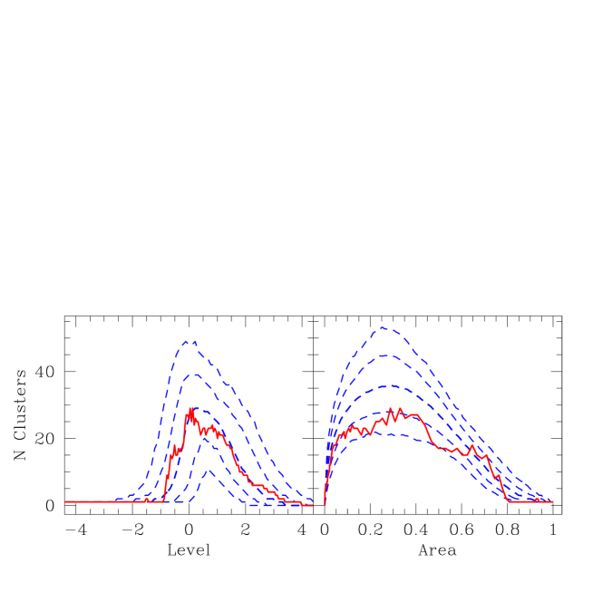
Figure 5: The number of regions $N_{c}$ as a function of the level $u={\Delta T}/\sigma_{{\Delta T}}$ (left hand panel) and as a function of $A$ (right hand panel). Other notation is as in Fig. 4

The number of isolated regions is shown in Fig. 5 for both the temperature and global area parameterizations. The latter is described in detail in Sec. 4.5.

In order to quantify the degree of non-Gaussianity of the QMASK map, we define and compute a functional that quantifies the “distance” between two functions in the functional space of measured statistics. The distance is defined by the integral

$$D_{ik}^{({\Delta T})} = \left\{\int_{-\infty}^{\infty}\left[M_{ik}({\Delta T})-\bar{M_{i}}({\Delta T})\right]^{2}~{}d({\Delta T})\right\}^{1/2},$$ (12)

$$i = 1,...,7;~{}~{}~{}k=1,...,1000$$ (13)

where

$$\bar{M_{i}}({\Delta T})=\frac{1}{1000}\sum_{k=1}^{1000}M_{ik}({\Delta T})$$ (14)

is the mean value of the statistic as a function of ${\Delta T}$. The integral in eq. (13) is approximated by the sum over a hundred levels of ${\Delta T}$. We also compute the distances of the each morphological curve from the Gaussian mean for the QMASK map. The third column of Table 1 shows the percentile of the QMASK map distances from the mean for each morphological statistic parameterized by ${\Delta T}$. The highest departure from the mean is shown by the $A({\Delta T})$ curve which is the cumulative probability function. It shows that only about 27% of Gaussian curves are closer to the Gaussian mean than the QMASK curve. Other parameters are even closer to the corresponding Gaussian mean.

4.5 Parameterization by the total area $A$.

The parameterization of the morphological parameters by the level of the field $u$ has serious drawbacks mentioned in Introduction. Although the parameterization by $\nu_{A}$ used in most studies of the genus is free of these drwbacks it seems to be more natural for morphological studies to use the total area $A({\Delta T})=A_{ES}({\Delta T})/A_{m}$ (where $A_{ES}({\Delta T})$ is the area of the excursion set at ${\Delta T}$ and $A_{m}\equiv A_{ES}(-\infty)$ is the total area of the map) as an independent parameter (Yess and Shandarin, 1996). It is one of the Minkowski functionals measured for the map, it represents the cumulative distribution functions of the field, and in addition it has a very simple geometrical interpretaaiton. It also has an additional advantage of decorrelating different statistics as discussed bellow. The $\nu_{A}$ parameterization must have similar properties because it is related to $A$ by a monotonic transform (the first eq. of 8).

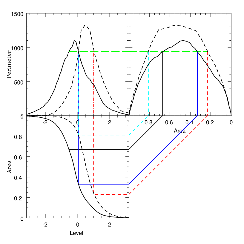
Figure 6: Illustration of the transformation from ${\Delta T}$ to $A$ parameterization. The thick solid lines show $C=C({\Delta T})$ (top left panel) $C=C(A)$ (top right panel) and $A=A({\Delta T})$ (bottom left panel) for the QMASK map. The thin solid lines illustrate the transformation. The dashed lines show similar transformation for a randomly chosen Gaussian map.

The transformation from the level parameterization to the area parameterization is a highly nonlinear procedure illustrated in Fig. 6. The thick lines correspond to the QMASK map (solid) and a randomly chosen Gaussian map (dashed). The transformation from $C({\Delta T})$ to $C(A)$ involves the $A({\Delta T})$ function shown in the lower panel, which is different for each map. The thin solid lines show the transformation for the QMASK map and dashed lines for the Gaussian map. Note that in order to illustrate this transformation, we reversed the $A$ axis in the $C=C(A)$ plot.

As an illustration of the diference between the level and area parameterization consider a simple example of a strong nonlinear field. Let the field $w(x,y)$ is the exponent of a Gaussian field $u(x,y)$: $w=\exp(\alpha u)$. The global Minkowski functionals of such a field can be easily derived from eq. 8

$$A(w) = \frac{1}{2}\left[1-{\rm erf}\left(\frac{\ln w}{\alpha\sqrt{2}}\right)\right],$$ (15)

$$C(w) = \frac{1}{2R}\exp\left(-\frac{(\ln w)^{2}}{2}\right),$$ (16)

$$G(w) = \frac{1}{(2\pi)^{\frac{3}{2}}}\frac{1}{R^{2}}(\ln w)\exp\left(-\frac{(\ln w)^{2}}{2}\right).$$ (17)

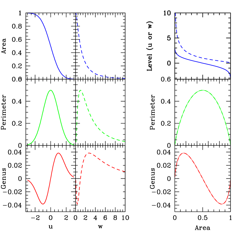
Figure 7: The global Minkowski functionals of the parent Gaussian field $u$ and derived non-Gaussian field $w=\exp u$ are shown in two left hand side panels as functions of the level. Both the perimeter and genus remain the same for both fields if they are parameterized by the total area (two bottom right hand side panels). All information about the non-Gaussianity of the $w$-field is stored in the cumulative probability function (dashed lines in the top panels). The solid lines in the top panels show the Gaussian cumulative probability function.

Fig. 7 illustrates the diference between the Minkowski functionals of the Gaussian field $u$ and non-Gaussian field $w$ (with $\alpha=1$) if both are parameterized by the level. The percolation curves differ strongly as well. On the other hand both the perimeter and genus as the functions of the area remain identical for the both fields because the transformation simply relabels the levels but does not affect the geometry of the contours. This is an example of a trivial non-Gaussian field when all non-Gaussian information is stored in the one-point probability density function. The further discussion of such fields can be found in Shandarin (2002).

Using the area parameterization, we compute seven new morphological functions for each map:

$$M_{i}(A)=[{\Delta T}(A),C(A),G(A),A_{p}(A),C_{p}(A),G_{p}(A),N_{c}(A)],~{}~{}~{}i=1,...,7.$$ (18)

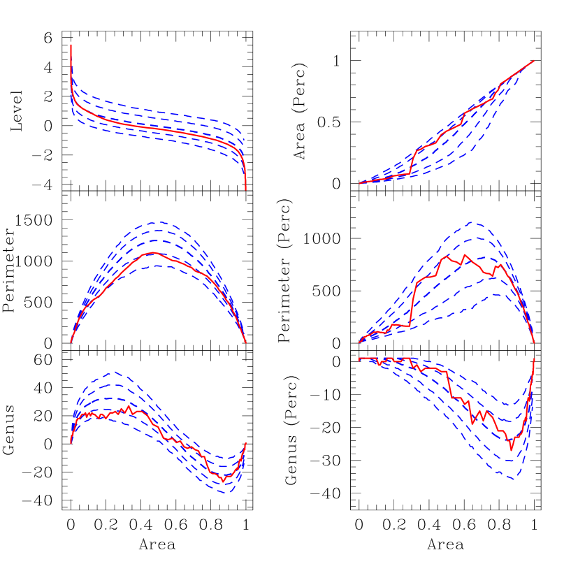
Figure 8: The figure is similar to Fig. 4, except that all morphological parameters are functions of $A=A_{ES}/A_{m}$, where $A_{ES}$ and $A_{m}=A_{ES}(-\infty)$ is the area of the excursion set and that of the whole map, respectively.

Figure 8 shows the measured quantities as functions of $A$. Similarly to Fig. 4 six panels show six Minkowski functionals measured for the QMASK map (solid lines) and the mean values for a thousand Gaussian maps (heavy dashed lines). The thin dashed lines show the 68% and 95% intervals.

The difference of the QMASK curves from the Gaussian mean is quantified similarly to that described before by the distance between curves in the functional space:

$$D_{ik}^{(A)} = \left\{\int_{0}^{1}\left[M_{ik}(A)-\bar{M_{i}}(A)\right]^{2}~{}dA\right\}^{1/2}$$ (19)

$$i = 1,...,7;~{}~{}~{}k=1,...,1000$$ (20)

where

$$\bar{M_{i}}(A)=\frac{1}{1000}\sum_{k=1}^{1000}M_{ik}(A).$$ (21)

There is an important difference between the two distances defined by eq. 13 and 20. Using $dA=-p_{k}({\Delta T})d({\Delta T})$ where $p_{k}({\Delta T})$ is the estimate of the probability function derived from the $k$-th map one can rewrite eq. 20 as an integral over ${\Delta T}$:

$$D_{ik}^{(A)} = \left\{\int_{0}^{1}\left[M_{ik}(A)-\bar{M_{i}}(A)\right]^{2}~{}dA\right\}^{1/2}$$ (22)

$$= \left\{\int_{-\infty}^{\infty}\left[M_{ik}({\Delta T})-\bar{M_{i}}({\Delta T})\right]^{2}p_{k}({\Delta T})~{}d({\Delta T})\right\}^{1/2}$$ (23)

Comparing eq. (13) and (23), one notices that the distance between the curves computed in the area space (eq. 20) depends more on the bulk of the probability function and less on the tails of the probability function, since it is weighted by the probability function. This obviously makes the measure more robust because the measurements at extreme levels are subject to large fluctuations. It is worth stressing that the calculation of all morphological parameters $M_{ik}$ themselves (eq. 11 and 18) is independent of the type of parameterization because $M_{ik}(A)\equiv M_{ik}({\Delta T})$ provided that $A$ is measured at corresponding ${\Delta T}$: $A=A({\Delta T})$. The only quantities that depend on the parameterization are the distances from the Gaussian expectation functions (eqs. 13 and 20) that are used for ranking the maps.

The second column of Table 1 shows the percentile of the QMASK distances from the mean in the area parameterization. Comparing the values corresponding to different parameterizations, one can easily see that the parameterization by ${\Delta T}$ suggests that the QMASK map is a more typical example of a Gaussian field than that using $A$ as an independent parameter. The parameterization by the level suggests that the most exceptional deviation of the QMASK map from Gaussianity is given by the $A({\Delta T})$ curve, but more than 70% of Gaussian maps differ from the mean more than the QMASK map. Thus, the QMASK map looks like a very typical realization of the Gaussian field. Parameterizing by the total area, one may conclude that the Gaussian $P(A)$ and $N_{c}(A)$ curves differ more than the QMASK map in only about 21% and 18% of the cases respectively. Thus, this parameterization reveals that the QMASK map is not quite a typical realization of the Gaussian field, but is not very unusual either, quite consistent with Gaussianity.

It is perhaps worth noting that all statistics but the genus of the percolating region, $G_{p}$ show a greater difference of the QMASK map with respect to the corresponding expectation value of the set of Gaussian maps in the $A$ parameterization than that in ${\Delta T}$ parameterization. Since the difference between two parameterizations for $G_{p}$ is not large (12% and 21%) it maybe a statistical fluctuation. One also may note that two columns of Table 1 appear anti-correlated. As we have discussed before the quantities shown in two columns of Table 1 have different sensitivity to the measurements at extreme ${\Delta T}$ levels both highest and lowest. The numbers in the first column corresponding to the $A$ parameterization are more robust.

4.6 Cross-correlations

The parameterization of the morphological statistics by the total area makes the set of parameters $M_{i}(A)$ (eq. 18) less correlated than $M_{i}({\Delta T})$ (eq. 11). Table 2 shows the correlation coefficients of the distances

$$r_{ij}=\frac{\sum\limits_{k=1}^{1000}(D_{ik}-\bar{D_{i}})(D_{jk}-\bar{D_{j}})}{\left[\left(\sum\limits_{k=1}^{1000}(D_{ik}-\bar{D_{i}})^{2}\right)\left(\sum\limits_{k=1}^{1000}(D_{jk}-\bar{D_{j}})^{2}\right)\right]^{1/2}}$$ (24)

for all 21 pairs of morphological statistics. The values above the diagonal show the correlations when all statistics were parameterized by the total area of the excursion set, $A$, while the values below the diagonal were computed using the parameterization by the level, ${\Delta T}$.

The correlation coefficient shows for each pair of statistics how well the separation from the mean Gaussian curve in one statistic $M_{i}$ can be predicted from the other one $M_{j}$. The closer $r_{ij}$ to unity, the less independent are corresponding statistics. In this respect the ${\Delta T}$ and $A$ parameterizations are very different. For instance, the lowest correlation in the class of the level parameterization is $0.82$ between $G_{p}({\Delta T})$ and $N_{c}({\Delta T})$ distances and 16 out of 21 cross-correlations are greater than $0.9$. In the class of the area parameterization, only one correlation coefficient is greater than $0.82$: that between $G(A)$ and $N_{c}(A)$ distances ($0.85$). Seventeen out of 21 pairs correlate at a level lower than $0.5$ thirteen of which at the level lower than $0.3$. Although absence of correlation does not prove the statistical independence of two sets of numbers, a correlation coefficient approaching unity indicates a strong statistical dependence.

5 Discussion

We present the results of a study of Gaussianity in the QMASK map. In agreement with the first study of topology of the degree-scale CMB anisotropy (Park et al., 2001), which was limited to the genus of QMASK, we conclude that the QMASK map is compatible with the assumption of Gaussian ${\Delta T}/T$ fluctuations. In this study, we used six morphological statistics in addition to the genus, $G$: the areas $A$ and $A_{p}$ of the excursion set and the largest (i.e. percolating) region, the contour lengths or perimeters $C$ and $C_{p}$ of the excursion set and the largest region; the genus $G_{p}$ of the percolating region and the number of isolated regions $N_{c}$. According to its morphology, the QMASK map is not a very typical example of a Gaussian field, but not very exceptional either: about 20% of a thousand Gaussian maps have greater differences with at least one mean function (Table 1).

We show that the parameterization of the morphological statistic is very important. A naive parameterization by the temperature threshold ${\Delta T}$ results in a highly correlated (almost degenerate) set of morphological characteristics: 16 out of 21 cross-correlation coefficients are greater than 0.9 and all the rest are greater than 0.82 (Table 2, bellow the diagonal). Representing the same morphological parameters as functions of the total area of the excursion set $A$ helps to decorrelate them: now 13 pairs correlate less than 0.3, four more correlate less than 0.5 and the rest less than 0.85 (Table 2, above the diagoanl).

Our measurements of the deviations of the morphological functions from the Gaussian mean strongly rely on the bulk of the probability function (see eq. 23) and therefore are robust to spurious effects.

In the $A$ parameterization the strongest deviations of the QMASK map from the Gaussian expectation values were shown by the number of peaks, $N_{c}(A)$ (82% i.e. the QMASK map deviates from the Gaussian expectation number of peaks more than 82% of Gaussian maps), total contour length of the excursion set, $C(A)$ (79%) and area of the percolating region, $A_{p}(A)$ (55%) while in the ${\Delta T}$ parameterization by the total area of the excursion set i.e. the cumulative probability function, $A({\Delta T})$ (27%), genus of the percolating region, $G_{p}({\Delta T})$ (21%) and contour length of the percolating region, $C_{p}({\Delta T})$ (20%).

The techniques that we have described here are computationally efficient ($\propto O(N_{pix}\ln N_{pix})$), and should be useful also for much larger upcoming datasets such as that from the MAP satellite. Another promising area for future applications is computing Minkowski functionals from foreground maps and topological defect simulations, thereby enabling quantitative limits to be placed on the presence of such structures in CMB maps.

6 Acknowledgment

Support for this work was provided by NSF grant AST00-71213, NASA grant NAG5-9194, the University of Pennsylvania Research Foundation, and the University of Kansas General Research Fund. HAF wishes to acknowledge support from the National Science Foundation under grant number AST-0070702 and the National Center for Supercomputing Applications. We wish also to thank the referee for a constructive criticism and useful suggestions.

Table 1: Percentage of Gaussian maps deviating less than QMASK.

	Parameterized by Area, $A$	Parameterized by Level, ${\Delta T}$
Level, ${\Delta T}$	28.2%
Area, $A$		27.2%
Perimeter, $C$	78.8%	6.1%
Genus, $G$	48.3%	2.0%
Area (Perc), $A_{p}$	54.6%	12.1%
Perimeter (Perc), $C_{p}$	24.3%	19.7%
Genus (Perc), $G_{p}$	11.6%	21.4%
Number of regions, $N_{c}$	82.5%	0.4%

Table 2: Correlations between different non-Gaussianity statistics parametrized by temperature, ${\Delta T}$ (below the diagonal) and area, $A$ (above the diagonal).

	$A$	$C$	$G$	$A_{p}$	$C_{p}$	$G_{p}$	$N_{c}$
${\Delta T}$		0.08	0.15	0.06	0.10	0.13	0.16
$C$	0.98	1	0.66	0.13	0.23	0.34	0.49
$G$	0.92	0.96	1	0.30	0.22	0.44	0.85
$A_{p}$	0.97	0.97	0.93	1	0.58	0.37	0.30
$C_{p}$	0.89	0.92	0.91	0.91	1	0.56	0.08
$G_{p}$	0.88	0.91	0.93	0.90	0.94	1	0.12
$N_{c}$	0.92	0.94	0.96	0.92	0.84	0.82	1

References

- Aghanim, Forni, and Bouchet (2001) Aghanim, N., Forni, O., and Bouchet, F.R. 2001, A&A,365, 341
- Banday, Zaroubi, and Górski (2000) Banday, A.J., Zaroubi, S., and Górski, K.R. 2000, ApJ, 533, 575
- Barreiro et al. (2000) Barreiro, R.b., Hobson, M.P., Lasenby, A.N., Banday, A.J., Górski, K.R., and Hinshaw, G. 2000, MNRAS, 318, 475
- Bharadwaj et al. (2000) Bharadwaj, S., Sahni, V., Sathyaprakash, B.S., Shandarin, S.F., and Yess, C. 2000, ApJ, 528, 21
- Bond and Jaffe (1998) Bond, J.R., Jaffe, A.H. 1998, in Proc. XVI Rencontre de Moriond, Microwave Background Anisotropies, ed. F. R. Bouchet (Paris: Editions Fronti res), 197
- Bromley and Tegmark (1999) Bromley, B. and Tegmark, M. 1999, ApJ, 524, L79
- Colley, Gott, and Park (1996) Colley, W.N., Gott, J.R., and Park, C. 1996, MNRAS, 281, L82
- Coles (1988) Coles, P. 1988, MNRAS, 234, 509
- Crofton (1968) Crofton, M.W. 1968, Phil.Trans.Roy.Soc. London 158, 181
- Devlin et al. (1998) Devlin, M., de Oliveira-Costa, A., Herbig, T., Miller, A.D., Netterfield, C.B., Page, L.A., and Tegmark, M. 1998, ApJ, 509, L77
- Dominik and Shandarin (1992) Dominik, K.G. and Shandarin, S.F., 1992, ApJ, 393, 450
- Ferreira, Magueijo, and Górski (1998) Ferreira P.G., Magueijo J., Górski K.M. 1998, ApJ, 503, L1
- Gott et al. (1990) Gott, III, J.R., Park, C., Juskiewicz, R., Bies, W.E., Bennett, D.P., Bouchet, F.R., Stebins, A. 1990, ApJ, 352, 1
- Hadwiger (1957) Hadwiger, H. 1957, Vorlesungen über Inhalt, Oberfläche und Isoperimetrie (Berlin: Springer)
- Herbig et al. (1998) Herbig, T., de Oliveira-Costa, A., Devlin, M.J., Miller, A.D., Page, L.A., and Tegmark, M. 1998, ApJ, 509, L73
- Kerscher (1999) Kerscher, M. 1999, astro-ph/9912329
- Kogut et al. (1996) Kogut, A., Banday, A.J., Górski, K.M., Hinshaw, G., Smoot, G.F., and Wright, E.L. 1996, ApJ, 464, L29
- Koenderink (1984) Koenderink, J.J. 1984, Biol. Cybern., 50, 363
- Magueijo (2000) Magueijo, J. 2000, ApJ, 528, L57
- Mecke, Buchert, and Wagner (1994) Mecke, K.R., Buchert, T, Wagner, H. 1994, A&A, 288, 697
- Mukherjee, Hobson, and Lasenby (2000) Mukherjee, P., Hobson, M.P., and Lasenby, A.N. 2000, MNRAS, 318, 1157
- Netterfield et al. (1995) Netterfield, C. B., Jarosik, N. C., Page, L. A., Wilkinson, D., and Wollack, E. J. 1995, ApJ, 445, L69
- Netterfield et al. (1997) Netterfield, C. B., Devlin, M. J., Jarosik, N., Page, L. A., and Wollack, E. J. 1997, ApJ, 474, 47
- Novikov, Feldman, and Shandarin (1999) Novikov, D., Feldman, H., and Shandarin, S.F. 1999, Int. J. of Mod. Phys. D8, 291
- de Oliveira-Costa et al. (1998) de Oliveira-Costa, A., Devlin, M., Herbig, T., Miller, A. D., Netterfield, C. B., Page, L. A., and Tegmark, M. 1998, ApJ, 509, L77
- Pando, Valls-Gabaud, and Fang (1998) Pando, J., Valls-Gabaud, D., and Fang, L.-Z. 1998, Phys. Rev. Lett., 81, 4568
- Park et al. (2001) Park, C-C., Park, C., Ratra, B., and Tegmark, M. 2001, astro/ph0102406
- Phillips and Kogut (2001) Phillips, N.G. and Kogut, A. 2001, ApJ, 548, 540
- Schmalzing and Buchert (1997) Schmalzing, J., and Buchert, T. 1997, ApJ, 482, L1
- Schmalzing and Górski (1998) Schmalzing, J., and Górski, K.M. 1998, MNRAS, 297, 355
- Shandarin (2002) Shandarin,S.F. 2002 MNRAS, 331, 865 (astro-ph/0107319)
- Shandarin (1983) Shandarin,S.F. 1983, Soviet Astron. Lett., 9, 104
- Shandarin and Yess (1998) Shandarin, S.F. and Yess, C. 1998, ApJ, 505, 12
- Shandarin and Zel’dovich (1989) Shandarin, S.F., and Zel’dovich, Ya.B. 1989, Rev. Mod. Phys., 61, 185
- Stauffer and Aharony (1992) Stauffer, D. and Aharony, A. 1992, Introduction to Percolation Theory, Taylor & Francis, London, Washington, DC.
- Tegmark (1997) Tegmark, M. 1997, Phys. Rev. D, 55, 5895
- Tegmark et al. (1996) Tegmark, M., de Oliveira-Costa, A., Devlin, M. J., Netterfield, C. B, Page, L. and Wollack, E. J. 1996 ApJ, 474, L77
- Turner (1997) Turner, M.S. 1997, in Generation of Cosmological Large-Scale Structure, eds. D.N. Schramm and P. Galeotti, Kluwer Academic Publishers, Dordrecht/Boston/London, p. 153
- Vilenkin and Shellard (1994) Vilenkin, A. and Shellard, P. 1994, Cosmic Strings and other Topological Defects. Cambridge University Press, Cambridge.
- Winitzki and Kosowsky (1997) Winitzki, S., and Kosowsky, A. 1997, New Astronomy, 3, 75
- Wu et al. (2001) Wu, J-H. P., Babul, A., Borrill, J., Ferreira, P.G., Hanany, S., Jaffe, A.H. Lee, A.T., Rabii, B., Richards, P.L., Smoot, G.F., Stompor, R., and Winant, C.D. 2001, astro-ph/0104248
- Xu et al. (2001) Xu, Y., Tegmark, M., de Oliveira-Costa, A., Devlin, M., Herbig, T., Miller, A.D., Netterfield, C.B., Page, L.A. 2001, PRD, 63, 103002
- Xu, Tegmark, and de Oliveira-Costa (2001) Xu, Y., Tegmark, M. and de Oliveira-Costa, A. 2001, astro-ph/0104419
- Yess and Shandarin (1996) Yess, C. and Shandarin, S. F. 1996, ApJ, 465, 2
- Zel’dovich, Mamaev, and Shandarin (1983) Zel’dovich, Ya.B., Mamaev, A.V., and Shandarin, S.F. 1983, Sov. Phys. Usp., 26, 77