M 33: A Galaxy with No Supermassive Black Hole

Abstract

Galaxies that contain bulges appear to contain central black holes whose masses correlate with the velocity dispersion of the bulge. We show that no corresponding relationship applies in the pure disk galaxy M 33. Three-integral dynamical models fit Hubble Space Telescope WFPC2 photometry and STIS spectroscopy best if the central black hole mass is zero. The upper limit is 1500 $M_{\odot}$. This is significantly below the mass expected from the velocity dispersion of the nucleus and far below any mass predicted from the disk kinematics. Our results suggest that supermassive black holes are associated only with galaxy bulges and not with their disks.

1. Introduction

The mass of a central black hole (BH) and the stellar orbital structure in a galaxy are direct probes into the formation and evolution history of both the galaxy and the BH. The tight correlation between BH mass $M_{\bullet}$ and bulge velocity dispersion $\sigma_{e}$ (Gebhardt et al. 2000a; Ferrarese & Merritt 2000) establishes a strong link between BHs and their hosts. Many theories (e. g., Silk & Rees 1998; Haehnelt & Kauffmann 2000; Ostriker 2000; Adams, Graff, & Richstone 2001) predict such a correlation. As data and theory improve, we hope to be able to discriminate between the alternatives.

The $M_{\bullet}$ – $\sigma_{e}$ correlation is derived using galaxies whose bulge-to-total luminosity ratios $B/T$ range from $\sim$ 0.15 to 1. They even include galaxies with “pseudobulges,” i. e., bulge-like, high-density central components that are believed to have grown by the secular evolution of disks (see Kormendy 1993 for a review). Bulges and pseudobulges appear to satisfy the same $M_{\bullet}$ – $\sigma_{e}$ correlation (Kormendy & Gebhardt 2001; Kormendy et al. 2001). However, the above references show that BHs do not correlate with the total gravitational potential of the disk. It therefore appears that the main requirement for a supermassive BH is that a galaxy contain some kind of bulge, or at least a mass gradient similar to one. Still, pure disk galaxies have not been studied in nearly the same detail as galaxies that contain bulges.

Observing pure disk galaxies is difficult, because they generally do not have bright centers and because the small expected BH masses require good spectral resolution. The presence of nuclei – compact star clusters that are distinct from the disk – have made it possible to study a few bulgeless galaxies. For example, based on its nuclear velocity dispersion, Filippenko & Ho (2001, see also Moran et al. 1999) conclude that the dwarf Seyfert galaxy NGC 4395 has $M_{\bullet}$ ${}_{<}\atop{{}^{\sim}}$ 80,000 $M_{\odot}$. However, a BH of only 100 $M_{\odot}$ is needed if the nucleus is radiating at the Eddington luminosity. Therefore NGC 4395 does not put a significant strain on the $M_{\bullet}$ – $\sigma_{e}$ correlation.

M 33 is the best bulgeless galaxy to use to investigate the relationship between BHs and disks. It is a normal, large galaxy (absolute magnitude $M_{V}=-19.0$), but it is only 0.8 Mpc away (van den Bergh 1991). The spatial scale is therefore unusually good, 0.^′′26 pc^-1. M 33 does not contain a bulge, but it does have a bright nucleus. Kormendy & McClure (1993) measured its velocity dispersion with the Canada-France-Hawaii Telescope and found that $\sigma=21\pm 3$ km s^-1. This implies an upper limit on the mass of any central black hole of $M_{\bullet}$ ${}_{<}\atop{{}^{\sim}}$ $5\times 10^{4}$ $M_{\odot}$. M 33 was the first large galaxy in which a dead quasar could strongly be ruled out. Recently, Lauer et al. (1998) obtained WFPC2 photometry and suggested that $M_{\bullet}$ ${}_{<}\atop{{}^{\sim}}$ $2\times 10^{4}$ $M_{\odot}$, by reducing the upper limits for the core radius of the nucleus. In this paper, we present Hubble Space Telescope (HST) STIS spectroscopy of the nucleus obtained with the 0.^′′1 slit. The spatial resolution is an order of magnitude better than that in Kormendy & McClure (1993). This leads to a much stronger limit on $M_{\bullet}$. Our best three-integral dynamical model has $M_{\bullet}$ = 0. Even our upper limit of 1500 $M_{\odot}$ is significantly below the value expected from the $M_{\bullet}$ – $\sigma_{e}$ correlation.

Figure 1.— Mean surface brightness profile of M 33 from Kormendy & McClure (1993) but with ground-based data inside 0.^′′5 replaced with HST photometry from Lauer et al. (1998). Their $V$- and $I$-band HST profiles have been used to synthesize the $R$-band profile plotted here.

It is important to emphasize how much M 33 differs from the galaxies in which BHs have been found. Figure 1 shows its brightness profile and Figure 1 in Kormendy & McClure (1993) shows an image of the central 70^′′ $\times$ 113^′′. There is no bulge; the exponential disk dominates the structure in to 3^′′. At the center, there is a compact nuclear star cluster that is dynamically distinct from the disk. At absolute magnitude $M_{B}=-10.2$, this is like a large globular cluster; it appears to be more closely related to globular clusters than to bulges in the Fundamental Plane parameter correlations (Kormendy & McClure 1993). The nucleus has a high central stellar density, similar to that of M 31 and M 32 (Kormendy & Richstone 1995; Lauer et al. 1998). But its velocity disperson is like that of a globular cluster, not like that of a bulge. Since mass $M\propto\sigma^{2}$, the difference in velocity dispersion is the essential reason why we find BHs in M 31 and M 32 but not in M 33.

2. Photometry

We use HST WFPC2 photometry from Lauer et al. (1998), who provide details of their reduction procedure. The bandpasses are $V$ and $I$, and the spatial resolution of the final profiles is 0.^′′025. Ground-based data at larger radii come from Kormendy & McClure (1993). There is a color gradient in the nucleus; its center is $\Delta\thinspace(V-I)=0.15$ bluer than its outer parts (Fig. 2). We want to measure the mass profile by using the light profile to represent the stellar potential, so we need to check how much the color gradient affects the results. It would be safest to use a $K$-band profile, because this would be least sensitive to the gradient in stellar population. Since we don’t have a $K$-band profile at the desired spatial resolution, we construct one by using the $V-I$ profile to estimate $V-K$. Giant stars have a monotonic and smooth relationship between $V-I$ and $V-K$ (Alves 2000, and references therein). At $V-I\simeq 1$ (appropriate for M 33), the relation is approximately linear, $\Delta$ $(V-K)=3\thinspace\Delta$ $(V-I)$. This relation provides the approximate $K$-band profile shown in Fig. 2. To further check the effect that color gradients have on the results, we have also run models where we change the mass-to-light ratio as a function of radius according to the $V-I$ profile; for these models we include a variation of 20% in the M/L_I starting from the edge of the nucleus decreasing linearly into the center. By either including a decrease in the mass-to-light ratio towards the center or using a flatter surface brightness profile (as suggested by the K-band profile), we are increasing the likelihood of requiring a black hole. Our goal is to place a robust and conservative upper limit on the black hole mass. Dynamical models constructed using the measured $V$, measured $I$, extrapolated $K$ profiles, and $I$ with varying M/L_I profiles all give very similar results. We conclude that the stellar population gradient does not have a significant affect on our estimates of $M_{\bullet}$. We discuss the results from each of the profiles below.

Surface brightness profiles of the nucleus of M 33. The $V$-band profile is the solid line, $I$-band is the dashed line, and $K$-band is the dotted line. We added 1.0 to the $I$-band profile and 2.32 to the $K$-band profile to match them at large radii. The bluer-light profiles are steeper in the middle.

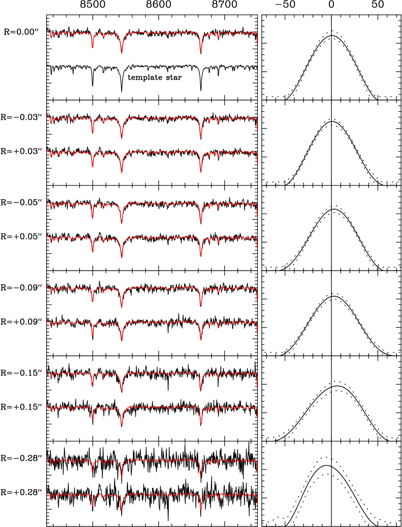
Figure 2.— M 33 spectra and velocity profiles. Each panel at left shows two radial bins. The black line is the galaxy spectrum used in the kinematic analysis. The red line is the spectrum of the template star convolved with the velocity profile. The top panel also shows the template star spectrum. The panels at right show the velocity profiles and their 68 % confidence bands.

Table 1Kinematics of the Nucleus of M 33

Radius	Velocity	$\sigma$	$h_{3}$	$h_{4}$
(arcsec)	($\rm{km}~{}\rm s^{-1}$)	($\rm{km}~{}\rm s^{-1}$)
0.00	$0.4\pm 1.4$	$23.9\pm 1.7$	$-0.00\pm 0.03$	$-0.04\pm 0.01$
0.03	$1.1\pm 1.1$	$22.0\pm 1.3$	$0.02\pm 0.03$	$-0.05\pm 0.01$
0.05	$2.1\pm 1.3$	$22.0\pm 1.4$	$-0.04\pm 0.03$	$-0.05\pm 0.01$
0.09	$2.7\pm 1.4$	$24.0\pm 1.6$	$0.00\pm 0.02$	$-0.04\pm 0.01$
0.15	$4.3\pm 2.3$	$24.7\pm 2.4$	$-0.02\pm 0.03$	$-0.06\pm 0.02$
0.28	$1.5\pm 4.4$	$18.9\pm 4.0$	$0.05\pm 0.04$	$-0.06\pm 0.03$
0.00	$0.0\pm 2.5$	$21.0\pm 3.0$	$\cdots$	$\cdots$
1.00	$8.0\pm 2.2$	$27.0\pm 3.0$	$\cdots$	$\cdots$

Note. — The bottom two lines are ground-based measurements by Kormendy & McClure (1993). They present only velocities and dispersions; we use these with Gaussian LOSVDs in the modeling.

3. HST STIS Kinematics

We measured the kinematics using the Space Telescope Imaging Spectrograph (STIS; Woodgate et al. 1998) centered at 8561 Å. Six exposures at three different pointings had a total exposure time of 2.05 hours. The 0.^′′1 $\times$ $52\arcsec$ slit and G750M grating provided pixels of 0.^′′05 $\times$ 0.55 Å = 19 $\rm{km}~{}\rm s^{-1}$. The nucleus of M 33 is slightly elongated (axial ratio $\simeq$ 0.85, Lauer et al. 1998); we put the slit along the major axis. Contemporaneous flats were used to remove pixel-to-pixel sensitivity variations and fringing. We did not use the weekly dark frames provided by STScI, because hot pixels come and go on timescales shorter than a day. Instead, we created a dark frame from the data using the iterative procedure described in Pinkney et al. (2001). The M 33 procedure differed slightly from normal: we have only 3 dither positions instead of 5, and the dither spacing is 4 pixels instead of 20. The steepness of the nuclear brightness profile alleviates the light overlap problem caused by the small dither spacing. It takes 5 iterations to bring the residual galaxy light level below 1 % of the initial value, i. e., acceptably below the noise. This process was used to create the dark frame that was subtracted from the galaxy spectra.

The STIS spectra are well sampled in the spatial direction, so it was possible to combine the dithered spectra without aliasing or the introduction of any artifacts or smoothing that would degrade the spatial resolution (Lauer 1999). We also choose to resample the spectra in the spatial direction to provide the greatest flexibility in sampling the kinematic parameters as a function of radius. Combination of the spectra began with shifting the spectra to a common spatial centroid to enable identification and elimination of cosmic ray events. Cosmic ray events in one spectrum were replaced with an average from the remaining spectra. The “cleaned” spectra were then shifted to a common centroid using sinc function interpolation. This allows well-sampled functions to be reinterpolated without the introduction of smoothing. The final composite spectrum was sampled with 0.^′′025 pixels. We also used a cruder combination of the data that set the pixel scale at 0.^′′05 pixels; in that case we find an upper limit on the black mass that is a factor of two larger. Thus, the resampling procedure is critical as it allowed superior use of the spatial information present in the data.

The galaxy spectrum was radially binned according to the optimal binning scheme used in the modeling. That is, the observations and models have the same radial bins. We use nearly linear bins at small radii and logarithmic bins at large radii (see Richstone et al. 2001 for details). The reduction procedure discussed in Pinkney et al. (2001) was then applied to the extracted spectra. Each spectrum was divided by an estimate of its continuum. This was based on binned windows from which we measured a robust mean (the biweight) using the highest 1/3 of the points. We then linearly interpolated between the mean values. The continuum division removes the need to flux calibrate the spectra.

Obtaining the internal kinematic information requires a deconvolution of the observed galaxy spectrum with a representative set of template stellar spectra. Both the deconvolution procedure and the choice of templates stars affect the derived velocity profiles. For the template, we use the K giant star HR7615. M 33 has younger stars near its center than farther out in the nucleus, so using using only a K III standard star may not be appropriate. In fact, M 33’s nucleus clearly contains A stars (Gordon et al. 1999, and references therein). Fortunately, the Ca triplet region is not as sensitive to template variations as is the more traditional Mg spectral region (Dressler 1984). M 33 shows a small radial variation in Ca triplet equivalent width from 10 Å at the center to 8 Å at 0.^′′5. Our template star, HR7615, has a Ca triplet equivalent width of 8 Å. García-Vargas et al. (1998) show that such a small difference in equivalent width has a small effect on age and metalicity. In Section 5, we discuss the possibility of this equivalent width difference affecting the deduced kinematics.

For the deconvolution, we reduce each spectrum using a maximum-penalized-likelihood (MPL) technique that produces a non-parametric line-of-sight velocity distribution (LOSVD). First, we guess initial velocity profiles in bins. We convolve these profiles with the template and calculate the residuals from the galaxy spectra. The program then varies the velocity profile parameters – i. e., the bin heights – to provide the best match to the galaxy spectrum. The MPL technique is similar to that used in Saha & Williams (1994) and in Gebhardt et al. (2000b). The complete set of spectra and velocity profiles are shown in Figure 3.

Our models are axisymmetric, so at any absolute radius $|r|$, they have the same LOSVDs on opposite sides of the center, except for the sign of the velocity. Thus, in order to maximize the signal-to-noise ratios in our observations, we fit the same velocity profile shape to both sides of the galaxy. In Figure 3, we plot these velocity profiles together with the two spectra at $\pm\thinspace|r|$. We have also measured the kinematics without symmetrizing. As expected, we obtain similar results but with larger uncertainties. Since we are trying to extract maximum information given low signal-to-noise levels in some spectra, the symmetrized versions are preferred.

Monte Carlo simulations are used to measure the uncertainties in the velocity profiles. We convolve the template star with the measured LOSVD to fit to the galaxy spectrum as illustrated by the red line in Figure 3. From this synthetic galaxy spectrum, we then generate 100 simulated observed spectra with noise, and we determine their velocity profiles. Each simulated spectrum contains random Gaussian noise with the standard deviation given by the RMS of the initial fit. The 100 simulated spectra and reductions provide a distribution of LOSVDs from which we estimate the confidence bands. The dashed lines in the right panels of Figure 3 represent the 68 % confidence bands of the distributions. This bootstrap techniques estimates both the random error and the bias of the estimator; however for these profiles the bias is negligible. We do not test for the bias due to template mismatch, but only estimator bias. The modeling described below uses these velocity profiles directly; we do not use a parametric representation of them. However, for convenience, Table 1 provides parameters and uncertainties of Gauss-Hermite fits to the velocity profiles.

Gebhardt et al. (2000a) use the luminosity-weighted velocity dispersion integrated out to the half-light radius of the bulge to define the “effective dispersion”. Here, we follow the same procedure for the nucleus. Integrating the STIS spectra from the center to the edge of the nucleus, we find an effective velocity dispersion of $\sigma_{e}=24.0\pm 1.2$ $\rm{km}~{}\rm s^{-1}$.

4. Three-Integral Models

The 3-integral models are the same as in Gebhardt et al. (2000b) and are described in detail in Richstone et al. (2001). The models are orbit-based (Schwarzschild 1979) and constructed using maximum entropy (Richstone & Tremaine 1988). We run a representative set of orbits in a specified potential and determine the non-negative weights of the orbits to best fit the available data. The library of orbits is convolved with the STIS PSF (as in Bower et al. 2001) and binned according to the STIS pixels. Maximizing the entropy helps to provide a smooth phase-space distribution function. Rix et al. (1997) present a similar code which has been applied to the spherical case; Cretton et al. (1999) and van der Marel et al. (1998) developed a fully-general axisymmetric code that is also orbit-based.

Because of M 33’s small dispersion and size we did not use the standard setup parameters as in Pinkney et al. (2001). Instead, we designed the model bins to include the high-resolution sampling that we used for the kinematic measurements. The central bins are 0.^′′025 wide.

The model consists of 15 radial, 5 angular, and 13 velocity bins. However, the force calculations use 4 times finer spatial sampling in order to achieve energy conservation to better than 1% for most stars. On average, each model contains about 3500 stellar orbits. We tried a variety of inclinations for the nucleus from edge-on to nearly face-on. In all cases we find a similar upper limit for the black hole mass. Zaritsky, Elston, & Hill (1989) measure an inclination of 56° for the disk.

The data consist of six HST radial bins and two ground-based bins with 13 velocity bins each. However, the actual number of independent measurements is less than 13 $\times$ 8, for several reasons. First, the ground-based measurements add only six independent values: a velocity and a dispersion at each of two positions. Second, each STIS pixel is 19 $\rm{km}~{}\rm s^{-1}$. Given the 120 $\rm{km}~{}\rm s^{-1}$ region where the velocity profile is non-zero, this implies about 6 independent measurements. Third, the smoothing length in the LOSVD estimate correlates some of the points. Thus, we have roughly 5 independent measurements per the six HST velocity profiles combined with the 4 ground-based measurements, giving about 34 degrees of freedom.

$\chi^{2}$ value as a function of black hole mass using the $I$-band light for the stellar potential. The points represent the models that we ran. The zero BH mass model is shown as an arrow.

5. Results

For each of the three light profiles, we ran nine models with BH masses ranging from zero to $1\times 10^{4}\,M_{\odot}$. The total $\chi^{2}$ values are shown in Figure 4 as a function of BH mass using the $I$-band light profile. For each BH mass, the best-fitting constant stellar $M/L$ ratio is 0.70 in $I$ band. Figure 4 only shows the one-dimensional $\chi^{2}$ values, and we do not plot these as a function of $M/L$ since there is little information there. The minimum $\chi^{2}$ value is around 27, which makes the reduced $\chi^{2}$ near unity.

Zero BH mass provides the best fit. Figure 4 only shows the results for the $I$ band where we have allowed the M/L_I to vary by 20%, but using any of the other light profiles also results in a minimum at zero BH mass. The difference between the various light profiles is in the upper limit for the black hole mass. For the $I$ band profile with varying M/L_I, $\Delta\chi^{2}=1$ at 1400 $M_{\odot}$; for $I$ with constant M/L_I, the upper limit is 600 $M_{\odot}$; using the $K$ profile, the upper limit occurs at 1200 $M_{\odot}$. We generally use a $\Delta\chi^{2}$ equal to one to signify the extent of the viable models, but, in this case, given the uncertainty of the light profile we choose a conservative upper limit of 1500 $M_{\odot}$.

The first four Gauss-Hermite moments of the velocity profiles for both model and data. The points with error bars represent the data, with large circles the HST points and small circles the two ground-based measurements of mean and dispersion. There are two lines which represent models with black hole masses of zero (red) and 15000 (black) $M_{\odot}$. The point at the smallest radii is actually centered at radius equal to zero.

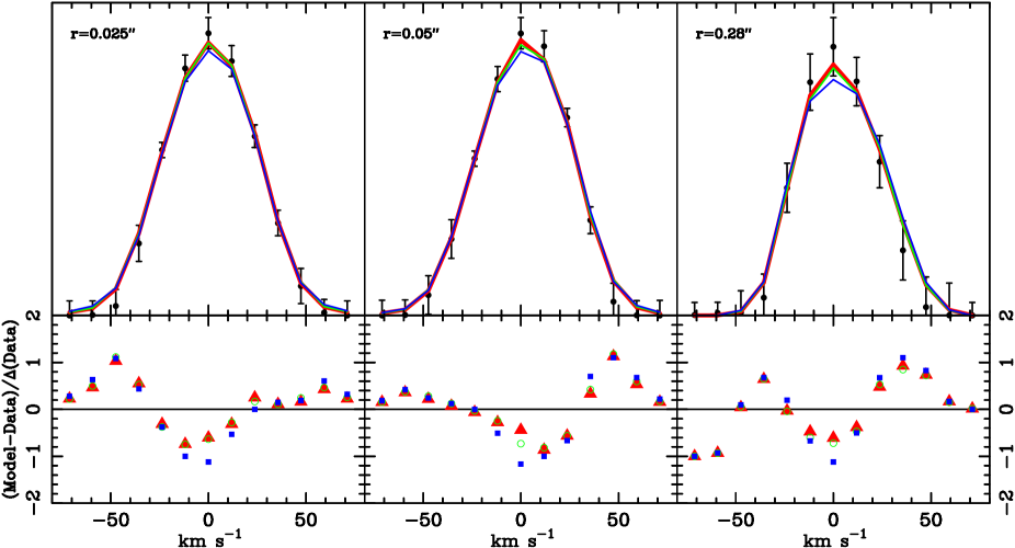
Figure 3.— The comparison of the LOSVD from three of the six STIS bins with model bins at radii as indicated. In the upper panels, the solid circles with error bars represent the data LOSVDs. The lines in the upper panel represent three different models, and the lower panel shows their normalized residuals from the data. The red line and triangles are the values from the zero BH model, the green line and open circles are the model with a 2000 $M_{\odot}$ BH, and the blue line and squares have a 7000 $M_{\odot}$ BH.

Figure 5 plots the first four Gauss-Hermite moments ($h_{3}$ and $h_{4}$ are measures of skewness and tail weight) of the velocity distributions for both model and data. There are two different BH models plotted in Figure 5, yet one would be very hard pressed to discern any difference between them. In fact, the difference in $\chi^{2}$ between the two models shown in Fig. 5 is 20, which significantly excludes the large black hole mass model. However, we do not use these Gauss-Hermite values during the fitting since the full LOSVD determines the $\chi^{2}$ minimization. Thus, it is not optimal to use these moments as a figure of merit to judge the quality of the fit. Instead, one should inspect the comparison with the velocity profiles. Figure 6 plots the LOSVD for three STIS bins with the same three BH models. The difference between the various models can now be seen. Furthermore, inspection of the other STIS velocity profiles reveal similar results—i.e., the model with no BH consistently provides the best fit. Only by looking at the total $\chi^{2}$ (Figure 4) can one judge the model fits.

The 3-Integral models also provide the stellar orbital distribution. In order to constrain adequately the stellar orbits, we must have two-dimensional spatial kinematic information. Major axis data allow for too large a parameter space for the models. Based on comparison with analytic models, the maximum entropy solution using only major kinematic axis data does not recover the input orbital distribution (Richstone et al. 2001). Having only one additional position angle helps considerably. Unfortunately, we only have major axis data for M 33 and so do not report the orbital structure. However, with only the major axis data, the estimate for the BH mass is unbiased.

5.1. Possible Problems

These 3-Integral models are limited by various assumptions. First, we assume that the nucleus is spheroidal (elliptical isophotes with ellipticity constant with radius). Second, the models are axisymmetric, so we do not consider triaxial shapes. Third, we assume specific radial forms for the $M/L$ variation. Any of these assumptions will reflect themselves as a bias in the models and restrict the measured uncertainties. The most important is likely the assumption of the $M/L$ variation. However, the color gradient is rather small ($\Delta{\thinspace}V-I=0.15$) and when we include a $M/L$ gradient, the results do not change significantly. This is apparent since we find similar results when we use the extrapolated $K$-band light profile.

No model can reproduce the $h_{4}$ values seen in the central few bins. We have thoroughly checked the negative $h_{4}$ values in these bins using extensive simulations to confirm that they are not an artifact of either the data analysis or velocity profile estimation. They appear to be a real feature in the data that is not reproducible in the models. The absolute difference between the model $h_{4}$ of $-0.02$ and the data $h_{4}$ of $-0.04$ is small but significant given the uncertainty. This difference may either be due to use of an improper template or to our lack of knowledge of the light distribution interior to our spatial resolution. Since M 33’s light profile is bluer in the center, template mismatch is likely since we are only using a K giant star. An A star will likely have a lower equivalent width for the Ca triplet, depending on the metalicity (García-Vargas et al. 1998); thus, if the center of M 33 consists of A stars, a fit using a higher equivalent width may result in an LOSVD with truncated wings, such as is seen. However, the absolute difference is so small (0.02) that it will have a negligible effect on our results.

Gordon et al. (1999) advocate a strong foreground of absorbing dust (V-band optical depth of 2), and we are not using an observed K-band light profile. Instead, we have estimated the K light using the V and I profiles. If the dust is distributed with a steep radial profile, then our K-band estimation will be in error. However, the effect is to make the upper black hole mass limit even tighter. As one includes more dust near the center, the result is to steepen the actual K-band profile and thereby increasing the amount of mass in the stellar component. Thus, unless the dust is distributed in a clever way, the upper limit that we derive on the black hole mass is robust.

We have assumed that the dynamical center of the galaxy is at the nucleus. Photometrically, the center of the galaxy is difficult to identify given the amount of dust; high spatial resolution IR imaging is required to determine the photometric center. X-ray observations (Colbert & Mushotzky 1999) show a compact source within 2″ of the nucleus, which is well within the ROSAT HRI uncertainty; but given that M33 does not appear to have a supermassive black hole, x-ray observations are unlikely to point to the galaxy center. Kinematically, the rotation curve is symmetric about the nucleus giving weight that we are looking at the galaxy center. However, the nature of the nucleus is unclear; it is similar to a large core-collapse globular cluster in both photometric and kinematic properties. Given the shallow potential well in the center of M33, such a dense system would be free to wander. Thus, even though there is no evidence to suggest a problem, a two-dimensional kinematic map of the nuclear region would be very useful to pinpoint the dynamical center.

6. Conclusions

The nuclear effective velocity dispersion of M 33 is $\sim$ 24 $\rm{km}~{}\rm s^{-1}$. If the mass of a central BH were related to this dispersion of a nucleus like the known BHs are related to the dispersions of their bulges; i. e., if $M_{\bullet}=1.3\times 10^{8}~{}(\sigma_{e}/200)^{3.65}$ (Gebhardt et al. 2001), then we would expect a BH of $M_{\bullet}=5.6\times 10^{4}$ $M_{\odot}$. The corresponding relationship from Ferrarese & Merritt (2000) implies a mass of 7000 $M_{\odot}$. The upper limit derived from the HST data is 1500 $M_{\odot}$ and the best-fit value is zero. Thus, M 33 appears to lie below the $M_{\bullet}$  – $\sigma_{e}$ correlation for bulges. This suggests that pure disk galaxies—even ones with nuclei—are different from bulges and ellipticals in their BH properties. Figure 7 plots M33’s upper limit in the $M_{\bullet}$  – $\sigma_{e}$ correlation. The line is given by the above relation and the 68% confidence bands are determined through a bootstrap procedure (Gebhardt et al. 2001).

The $M_{\bullet}$ – $\sigma_{e}$ correlation for the galaxies from Kormendy & Gebhardt (2001) including M33. The line is the best fit to the BH detections; the relation is given by $M_{\bullet}=1.3\times 10^{8}~{}M_{\odot}\left(\sigma_{e}/200~{}{\rm km~{}s^{-1}}\right)^{3.65}$. We have assumed for this plot that the bulge of M33 is its nucleus.

There is a caveat. Because there are no firm dynamical BH detections in the mass range $10^{3}$ to $10^{6}$ $M_{\odot}$, there is a big gap in the $M_{\bullet}$  – $\sigma_{e}$ correlation between the smallest known supermassive BHs and the mass limit in M 33. That is, we do not know whether the correlation extends down to the small masses of interest here; this is not a problem: our observation may be a sign that it does not. But given the large gap, we also do not know that the correlation—if it exists—is linear between $10^{6}$ and $10^{3}$ $M_{\odot}$. If the correlation exists but is not linear, then our limit of $M_{\bullet}$ ${}_{<}\atop{{}^{\sim}}$ 1500 $M_{\odot}$ may not be below the correlation. Furthermore, the confidence band in Figure 7 assumes a linear relation; thus, deviations from a linear relation will have a significant affect on the estimated uncertainties.

On the other hand, Kormendy et al. (2001) show that our $M_{\bullet}$ limit in M 33—and published masses and mass limits on BHs in other disk galaxies—are far below the correlation of $M_{\bullet}$ with the total luminosities of their host galaxies. M 33 is by far the most extreme case. There is a corresponding argument for the $M_{\bullet}$  – $\sigma_{e}$ correlation. The H I rotation curve of the outer disk of M 33 rises slowly from about 100 $\rm{km}~{}\rm s^{-1}$ at $r=15^{\prime}$ = 3.5 kpc to about 135 $\rm{km}~{}\rm s^{-1}$ at $r=77^{\prime}$ = 18 kpc (Corbelli & Salucci 2000). If these are circular velocities in the gravitational potential of an almost isothermal dark halo, then the corresponding one-dimensional velocity dispersion is $\sigma\sim 85\pm 10$ $\rm{km}~{}\rm s^{-1}$. If a BH in M 33 were related to the dark matter potential well like known BHs are related to their bulge potential wells (both represented by $\sigma_{e}$), then M 33 should contain a BH of mass $M_{\bullet}\sim 6\times 10^{6}$ $M_{\odot}$. Clearly it does not. If M 33 is typical of disk galaxies, then BH masses are not related in the same way to every gravitational potential well (as measured by $\sigma_{e}$). In particular, they are not related to the potential well of the disk and dark matter. Taken together, our results and those of Kormendy et al. (2001) strongly suggest that BH masses are causally connected with the properties—luminosity, mass, and especially velocity dispersion—of their host bulges and not with their disks.

These results are still based on only a few, well-observed galaxies. We therefore need to study the $M_{\bullet}$  – $\sigma_{e}$ correlation more fully at the low-dispersion end. This should provide further insight into the fundamental differences between disk and bulge galaxies, and it may help to tell us why such a correlation exists in the first place.

References

- (1)
- (2) Adams, F. C., Graff, D. S., & Richstone, D. O. 2001, ApJ, 551, L31
- (3) Alves, D. 2000, ApJ, 539, 732
- (4) Bower, G.A. et al. 2001, ApJ, 550, 75
- (5) Colbert, E. & Mushotzky, R. 1999, ApJ, 519, 89
- (6) Corbelli, E., & Salucci, P. 2000, MNRAS, 311, 441
- (7) Cretton, N., de Zeeuw, P. T., van der Marel, R. P., & Rix, H.-W., 1999, ApJS, 124, 383
- (8) Dressler, A. 1984, ApJ, 286, 97
- (9) Ferrarese, L., & Merritt, D. 2000, ApJ, 539, L9
- (10) Filippenko, A. V., & Ho, L. C. 2001, ApJ, in preparation
- (11) García-Vargas, M.L., Mollá, M., & Bressan, A. 1998, A&AS, 130, 513
- (12) Gebhardt, K. et al. 2000a, ApJ, 539, L13
- (13) Gebhardt, K. et al. 2000b, AJ, 119, 1157
- (14) Gebhardt, K. et al. 2001, in preparation
- (15) Gordon, K. D., Hanson, M. M., Clayton, G. C., Rieke, G. H., & Misselt, K. A. 1999, ApJ, 519, 165
- (16) Haehnelt, M. G., & Kauffmann, G. 2000, MNRAS, 318, L35
- (17) Kormendy, J. 1993, in IAU Symposium 153, Galactic Bulges, ed. H. Dejonghe & H. J. Habing (Dordrecht: Kluwer), 209
- (18) Kormendy, J., & Gebhardt, K. 2001, in The 20th Texas Symposium on Relativistic Astrophysics, ed. H. Martel & J. C. Wheeler (New York: AIP), in press (astro-ph/0105230)
- (19) Kormendy, J., & McClure, R. D. 1993, AJ, 105, 1793
- (20) Kormendy, J., & Richstone, D. 1995, ARA&A, 33, 581
- (21) Kormendy, J. et al. 2001, ApJ, submitted
- (22) Lauer, T. R. et al. 1998, AJ, 116, 2263
- (23) Lauer, T. R. 1999, PASP, 112, 227
- (24) Moran, E. C., et al. 1999, PASP, 111, 801
- (25) Ostriker, J. P. 2000, Phys. Rev. Lett., 84, 5258
- (26) Pinkney, J. et al. 2001, in preparation
- (27) Richstone, D. O., & Tremaine, S. 1984, ApJ, 286, 27
- (28) Richstone, D. O. et al. 2001, in preparation
- (29) Rix, H.-W., de Zeeuw, P. T., Cretton, N., van der Marel, R. P., & Carollo, C. M. 1997, ApJ, 488, 702
- (30) Saha, P., & Williams, T. B. 1994, AJ, 107, 129
- (31) Schwarzschild, M. 1979, ApJ, 232, 236
- (32) Silk, J., & Rees, M. J. 1998, A&A, 331, L1
- (33) van den Bergh, S. 1991, PASP, 103, 609
- (34) van der Marel, R. P., Cretton, N., de Zeeuw, P. T., & Rix, H.-W. 1998, ApJ, 493, 613
- (35) Woodgate, B.E., Kimble, R.A., Bowers, C.W., Kraemer, S., Kaiser, M.E., et al. 1998, PASP, 110, 1183
- (36) Zaritsky, D., Elston, R., & Hill, J.M. 1989, AJ, 97, 97
- (37)