Statistical Properties of DLAs and sub-DLAs

Abstract

Quasar absorbers provide a powerful observational tool with which to probe both galaxies and the intergalactic medium up to high redshift. We present a study of the evolution of the column density distribution, $f(N,z)$, and total neutral hydrogen mass in high-column density quasar absorbers using data from a recent high-redshift survey for damped Lyman-$\alpha$ (DLA) and Lyman limit system (LLS) absorbers. Whilst in the redshift range 2 to 3.5, $\sim$90% of the neutral HI mass is in DLAs, we find that at z$>$3.5 this fraction drops to only 55$\%$ and that the remaining ’missing’ mass fraction of the neutral gas lies in sub-DLAs with N(HI) $\rm 10^{19}-2\times 10^{20}~{}cm^{-2}$.

Institute of Astronomy, Madingley Road, Cambridge CB3 0HA, UK

SIRTF Science Center, CalTech, Pasadena, USA

1. Introduction

Intervening absorption systems in the spectra of quasars provide a unique way to study early epochs and galaxy progenitors. In particular, they are not affected by the “redshift desert” from $1.3\stackrel{{\scriptstyle<}}{{{}_{\sim}}}z\stackrel{{\scriptstyle<}}{{{}_{\sim}}}2.5$ where spectral emission features in normal galaxies do not fall in optical passbands, yet where substantial galaxy formation is taking place. In addition, the absorbers are selected strictly by gas cross-section, regardless of luminosity, star formation rate, or morphology. Quasar absorbers are divided according to their neutral hydrogen column densities: DLAs have N(HI) $>2\times 10^{20}$ cm^-2, Lyman-limit systems have N(HI) $>1.6\times 10^{17}$ cm^-2 and any system below this threshold is known as the Lyman-$\alpha$ forest. The analysis presented here is based on a sample of quasar absorbers found in the spectra of 66 $z\stackrel{{\scriptstyle>}}{{\sim}}4$ quasars (Peroux et al. 2001b) combined with data from the literature (Storrie-Lombardi & Wolfe 2000).

2. Quasar Absorbers Number Density and Column Density Distribution

The absorption lines evolution is usually described with a power law of the form: $n(z)dz=n_{0}(1+z)^{\gamma}dz$, where $n(z)$ is the observed number density of absorbers. For convenience, the $dz$ is dropped and the differential number density per unit redshift is expressed as follow: $n(z)=n_{0}(1+z)^{\gamma}$. The observed number density of absorbers is the product of the space density and physical cross-section of the absorbers which are a function of the geometry of the Universe. For no evolution of the properties of the individual aborbers in a ${\Lambda}=0$ Universe, this yields $\gamma=1$ for $\Omega_{M}=0$ and $\gamma=0.5$ for $\Omega_{M}=1$. We found $\gamma=2.45^{+0.75}_{-0.65}$ indicating evolution at the $\sim 2\sigma$ level independently of $\Omega_{M}$. Figure 1 shows the number density of various classes of quasar absorbers.

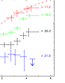
Figure 1.: Number density of quasar absorbers with (from top to bottom) log $N(HI)>17.2$, $>19.0$, $>20.3$ and $>21.0~{}cm^{-2}$. The column density range $10^{19}<N(HI)<10^{20.3}~{}cm^{-2}$ are not direct observations but re-computed from the $\Gamma$-fit to the column density distribution including the expected number of LLS. The dashed line is a power-law fit to the number density of LLS with $z_{abs}>2.4$. No absorber with log $N(HI)>21.0~{}cm^{-2}$ are observed at $z>4$ and the arrow indicates the $50\%$ confidence upper limit.

The column density distribution is determined as follow:

$$f(N,z)dNdX=\frac{n}{\Delta N\sum_{i=1}^{m}\Delta X_{i}}dNdX$$ (1)

where $n$ is the number of quasar absorbers observed in a column density bin $[N,N+dN]$ obtained from the observation of $m$ quasar spectra with total absorption distance coverage $\sum_{i=1}^{m}\Delta X_{i}$. The distance interval, $dX$, is used to correct to co-moving coordinates and thus depends on the geometry of the Universe. In a non-zero $\Lambda$-Universe:

$$X(z)=\int_{0}^{z}(1+z)^{2}\left[(1+z)^{2}(1+z\Omega_{M})-z(2+z)\Omega_{\Lambda}\right]^{-1/2}dz$$ (2)

The column density distribution was usually fitted by a power law over a large column density range $N(HI)$ $10^{12}-10^{21}$ cm^-2. This suggested that all classes of absorbers arise from the same cloud population (Tytler 1987). Assuming randomly distributed spherical isothermal halos, $f(N,z)$ was well approximated with a power law of slope $-5/3$ (Rees 1988). Nevertheless, as the quality of the data increased, deviations from a power law have been observed. In particular Petitjean et al. (1993) observed a change in slope: $\beta=-1.83$ for $N(HI)\leq 10^{16}$ and $\beta=-1.32$ above that threshold (Figure 2).

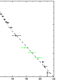
Figure 2.: Column density distribution, $f(N,z)$, at $z_{abs}>3.5$. The low column density data are Keck-HIRES observations of the Lyman-$\alpha$ forest (BR 1033$-$0327 and Q0000$-$26, Williger et al. 1994 and Lu et al. 1996, respectively). The light grey bins (in the range $17.2<$ log $N(HI)<20.3$) are deduced from the fit to the observed cumulative number of quasar absorbers. The turn-over at the low column density end is incompleteness due to a combination of spectral resolution and signal-to-noise. The dashed and dotted lines are the two $<z>\simeq 2.8$ power law fits from Petitjean et al. (1993) corrected for the absorber number density evolution with redshift and to $\Omega_{\Lambda}=0.7$, $\Omega_{M}=0.3$ cosmology.

However, LLS line profiles cannot be used to directly measure their column densities in the range $10^{17.2}$ to $10^{19.0}$ cm^-2 because the curve of growth is degenerate in that interval. In our analysis, we use the expected number of LLS to provide a further constraint on the cumulative number of quasar absorbers and as clear evidence that a simple power law does not fit the observations:

$$LLS_{expected}=\sum_{i=1}^{n}\int_{z_{min}}^{z_{max}}N_{o}(1+z)^{\gamma}dz$$ (3)

where $z_{min}$ and $z_{max}$ is the redshift path along which quasar absorbers were searched for. We choose to fit the data with a $\Gamma$-distribution (a power law with an exponential turn-over) which was introduced by Pei $\&$ Fall (1995) and Storrie-Lombardi, Irwin & McMahon (1996b):

$$f(N,z)=(f_{*}/N_{*})(N/N_{*})^{-\beta}e^{-N/N_{*}}$$ (4)

where $N$ is the column density, $N_{*}$ a characteristic column density and $f_{*}$ a normalising constant. Figure 3 shows the differential column density distribution of quasar absorbers with the $\Gamma$-distribution fit for various redshift ranges. The redshift evolution indicates that there are less high column density systems at high-redshift than at low redshift, confirming the earlier results from Storrie-Lombardi, McMahon & Irwin (1996a) and Storrie-Lombardi & Wolfe (2000). This suggests that we are observing the epoch of formation of DLAs.

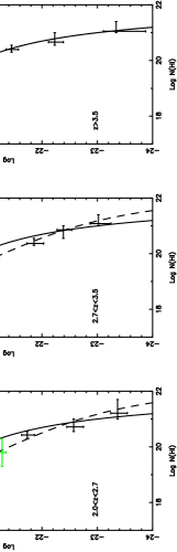
Figure 3.: Column density distribution of quasar absorbers for various redshift ranges. The redshift ranges are chosen to match the bins in the $\Omega_{HI+HeII}$ plot (see Figure 4). The light grey bins (in the range $17.2<$ log $N(HI)<20.3$) are deduced from the fit to the observed cumulative number of quasar absorbers. The solid line is the $\Gamma$-distribution fit for $z>3.5$ and the dashed lines are the fits to the unbinned data in the relevant redshift range.

3. Cosmological Evolution of Neutral Gas Mass

The mass density of absorbers can be expressed in units of the current critical mass density, $\rho_{crit}$, as:

$$\Omega_{HI+HeII}(z)=\frac{H_{o}\mu m_{H}}{c\rho_{crit}}\int_{N_{min}}^{\infty}Nf(N,z)dN$$ (5)

where $\mu$, the mean molecular weight is $1.3$ and $m_{H}$ is the hydrogen mass. The total HI may be estimated as:

$$\int_{N_{min}}^{\infty}Nf(N,z)dN=\frac{\sum N_{i}(HI)}{\Delta X}$$ (6)

If a power law is used to fit $f(N,z)$, up to $90\%$ of the neutral gas is in DLAs (Lanzetta, Wolfe & Turnshek 1995), although an artificial cut-off needs to be introduced at the high column density end because of the divergence of the integral. If instead a $\Gamma$-distribution is fitted to $f(N,z)$ this removes the need to artificially truncate the high end column distribution and can be used to probe in more detail the neutral gas fraction as a function of column density and how this changes with redshift. The resulting $\Omega_{HI+HeII}$ is shown in Figure 4.

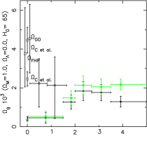
Figure 4.: The black circles show the neutral gas in Damped Lyman-$\alpha$ galaxies in a $\Omega_{\Lambda}=0.7$, $\Omega_{M}=0.3$ and $h=0.65$ Universe (left panel). Vertical error bars correspond to 1-$\sigma$ uncertainties and the horizontal error bars indicate bin sizes. The light grey stars are the total HI+HeII including a correction for the neutral gas contained in sub-DLAs. The circles at low redshift are the measurements from Rao $\&$ Turnshek (2000), who used a method involving the observations of quasar spectra with known MgII systems. The triangle at $z=0$ is the local HI mass measured by Natarajan $\&$ Pettini (1997). The squares, $\Omega_{FHP}$, $\Omega_{GO}$ and $\Omega_{Cetal.}$ (Fukugita, Hogan $\&$ Peebles 1998, Gnedin $\&$ Ostriker 1992 and Cole et al. 2000 respectively) are $\Omega_{baryons}$ in local galaxies. The right panel is for a $\Omega_{M}=1$ cosmology. This plot shows that the geometry of the Universe affects the absolute value of $\Omega_{HI+HeII}$ with respect to the local $\Omega_{baryons}$.

4. Results and Discussion

We find that at z$>$3.5 the fraction of mass in DLAs is only 55$\%$ and that the remaining fraction of the neutral gas mass lies in systems below this limit, in the so-called “sub-DLAs” with column density $10^{19}<$ N(HI) $<2\times 10^{20}$ cm^-2 (Peroux et al. 2001a). Our observations in the redshift range 2 to 5 are consistent with no evolution in the total amount of neutral gas. Under simple assumptions of closed box evolution, his could be interpreted as indicating there is little gas consumption due to star formation in DLA systems in this redshift range. Similarly, at z $>$ 2, Prochaska, Gawiser & Wolfe (2001) conclude that there is no evolution in the metallicity of DLA systems from column density-weighted Fe abundance measurements in DLAs (see also Savaglio 2000). At low-redshift, recent measurements of $\Omega_{HI+HeII}$ by Rao & Turnshek (2000) at $z\stackrel{{\scriptstyle<}}{{\sim}}1.65$ and Churchill (2001) at $z\sim 0.05$ are difficult to reconcile with 21 cm emission observations at $z=0$. Nevertheless, the cosmological evolution of the total neutral gas mass proves to be a powerful way of tracing galaxy formation with redshift: it probes the epoch of assembly of high column density systems from lower column density units.

Acknowledgments.

CP would like to thank the organising committee for putting together a very enjoyable meeting.

References

Churchill, C., 2001, ApJ, (astro-ph/0105044)

Cole, S. & the 2dFRGS team, 2000, MNRAS, (astro-ph/0012429)

Fukugita, M., Hogan, C. & Peebles, P., 1998, ApJ, 503, 518

Gnedin, N. & Ostriker, J., 1992, ApJ, 400, 1

Lanzetta, K., Wolfe, A. & Turnshek, D., 1995, ApJ, 440, 435

Lu, L., Sargent, W., Womblem D. & Takada-Hidai, M., 1996, ApJ, 472, 509

Natarajan, P. & Pettini, M., 1997, MNRAS, 291, 28

Pei, Y. & Fall, M., 1995, ApJ, 454, 69

Peroux, C., McMahon, R. G., Storrie-Lombardi, L. J., & Irwin. M. J. 2001b, MNRAS, (astro-ph/0107045)

Peroux, C., Storrie-Lombardi, L. J., McMahon, R. G., Irwin. M. J. & Hook, I. M. 2001a, AJ, 121, 1799

Petitjean, P., Webb, J., Rauch. M., Carswell, R., & Lanzetta, K., 1993, MNRAS, 262, 499

Prochaska, J., Gawiser, E. & Wolfe, A., 2001, ApJ, in press, (astro-ph/0101029)

Rao, S. & Turnshek, D., 2000, ApJS, 130, 1

Rees, M. 1988, Cambridge University Press, Vol. 107

Savaglio, S., 2000, IAU Symposium, Vol. 204

Storrie-Lombardi, L., Irwin, M. &McMahon, R. 1996a, MNRAS, 282, 1330

Storrie-Lombardi, L., McMahon, R. & Irwin, M., 1996b, MNRAS, 283, L79

Storrie-Lombardi, L. & Wolfe, A., 2000, ApJ, 543, 552

Tytler, D., 1987, ApJ, 321, 68

Williger, G., Baldwin, J., Carswell, R., Cooke, A., Hazard, C., Irwin, M., McMahon, R., & Storrie-Lombardi, L., 1994, ApJ, 428, 574