[

Correlated perturbations from inflation and the cosmic microwave background

Abstract

We compare the latest cosmic microwave background data with theoretical predictions including correlated adiabatic and CDM isocurvature perturbations with a simple power-law dependence. We find that there is a degeneracy between the amplitude of correlated isocurvature perturbations and the spectral tilt. A negative (red) tilt is found to be compatible with a larger isocurvature contribution. Estimates of the baryon and CDM densities are found to be almost independent of the isocurvature amplitude. The main result is that current microwave background data do not exclude a dominant contribution from CDM isocurvature fluctuations on large scales.

]

Increasingly accurate measurements of temperature anisotropies in the cosmic microwave background sky offer the prospect of precise determinations of both cosmological parameters and the nature of the primordial perturbation spectra. The recent Boomerang [1], DASI [2] and Maxima [3] data have shown evidence for three peaks in the cosmic microwave background (CMB) temperature anisotropy power spectrum as expected in inflationary scenarios. In this context the CMB data support the current ‘concordance’ model based on a spatially flat Friedmann-Robertson-Walker universe dominated by cold dark matter and a cosmological constant [4]. In addition, the CMB data no longer shows any signs of being in conflict with the big bang nucleosynthesis data [5].

In the studies which have estimated the cosmological and primordial parameters with these new data sets, only the case of purely adiabatic perturbations has been considered so far. That is, the perturbation in the relative number densities of different particle species is taken to be zero. Although this assumption is justified for perturbations originating from single field inflationary models, it does not necessarily follow when there is more than one field present during inflation [6, 7, 8, 9, 10]. Other possible primordial modes are isocurvature [11, 12] (also referred to as “entropy”) modes in which the particle ratios are perturbed but the total energy density is unperturbed in the comoving gauge.

Most previous studies have examined the extent to which a statistically independent isocurvature contribution to the primordial perturbations may be constrained by CMB and large-scale structure data [13, 14]. It has recently been shown that multi-field inflationary models in general produce correlated adiabatic and isocurvature perturbations [7, 8, 9, 10]. These correlations can dramatically change the observational effect of adding isocurvature perturbations [15, 12]. Up until now, only the case of scale-invariant correlated adiabatic and entropy perturbations has been considered. Trotta et al. [16] found (with an earlier CMB dataset) that in this case the cold dark matter (CDM) isocurvature mode was likely to be very small if not entirely absent, though they did find that a neutrino isocurvature mode contribution [12] was not ruled out. In this letter we examine to what extent a correlated CDM isocurvature mode is consistent with the recent CMB data when a tilted power law spectrum is allowed.

Non-adiabatic perturbations are produced during a period of slow-roll inflation in the presence of two or more light scalar fields, whose effective masses are less than the Hubble rate. On sub-horizon scales, fluctuations remain in their vacuum state so that when fluctuations reach the horizon scale their amplitude is given by $\hat{\delta\phi}_{i*}\simeq\left({H_{*}/2\pi}\right)\hat{a}_{i}$ where the subscript $*$ denotes horizon-crossing and $\hat{a}_{i}$ are independent normalised Gaussian random variables, obeying $\langle\hat{a}_{i}\hat{a}_{j}\rangle=\delta_{ij}$. The total comoving curvature and entropy perturbation at any time during two-field inflation can quite generally be given in terms of the field perturbations, along and orthogonal to the background trajectory, as [8]

$$\hat{\cal R} \propto \cos\theta\,\hat{\delta\phi}_{1}+\sin\theta\,\hat{\delta\phi}_{2}\,,$$ (1)

$$\hat{\cal S} \propto -\sin\theta\,\hat{\delta\phi}_{1}+\cos\theta\,\hat{\delta\phi}_{2}\,,$$ (2)

where $\theta$ is the angle of the inflaton trajectory in field space. Although the curvature and entropy perturbations are uncorrelated at horizon-crossing, any change in the angle of the trajectory, $\theta$, will begin to introduce correlations [8]. Further correlations may be introduced by the model dependent dynamics when inflation ends and the fields’ energy is transformed into radiation and/or dark matter. The comoving curvature perturbation, ${\cal R}_{\rm rad}$, on large-scales during the radiation-dominated era is related to the conformal Newtonian metric perturbation, $\Phi$, by ${\cal R}_{\rm rad}=3\Phi/2$. The isocurvature perturbation is ${\cal S}_{\rm rad}=\delta\rho_{\rm cdm}/\rho_{\rm cdm}-(3/4)\delta\rho_{\gamma}/\rho_{\gamma}$ and remains constant on large scales until it re-enters the horizon. On large scales the CMB temperature perturbation can be expressed in terms of the primordial perturbations [7]

$$\frac{\hat{\delta T}}{T}\approx\frac{1}{5}\left(\hat{{\cal R}}_{\rm rad}-2\hat{{\cal S}}_{\rm rad}\right)\,.$$ (3)

The general transformation of linear curvature and entropy perturbations from horizon-crossing during inflation to the beginning of the radiation era will be of the form

$$\left(\begin{array}[]{c}\hat{\cal R}_{{\rm rad}}\\ \hat{\cal S}_{{\rm rad}}\end{array}\right)=\left(\begin{array}[]{cc}1&T_{{\cal R}{\cal S}}\\ 0&T_{{\cal S}{\cal S}}\end{array}\right)\left(\begin{array}[]{c}\hat{\cal R}_{*}\\ \hat{\cal S}_{*}\end{array}\right)\,,$$ (4)

Two of the matrix coefficients, $T_{{\cal R}{\cal R}}=1$ and $T_{{\cal S}{\cal R}}=0$, are determined by the physical requirement that the curvature perturbation is conserved for purely adiabatic perturbations and that adiabatic perturbations cannot source entropy perturbations on large scales [17]. The remaining terms will be model dependent. If the fields and their decay products completely thermalize after inflation then $T_{{\cal S}{\cal S}}=0$ and there can be no entropy perturbation if all species are in thermal equilibrium characterised by a single temperature, $T$. This means that it is unlikely that a neutrino isocurvature perturbation could be produced by inflation unless the reheat temperature is close to that at neutrino decoupling shortly before primordial nucleosynthesis takes place. On the other hand, a cold dark matter species could remain decoupled at temperatures close to, or above, the supersymmetry breaking scale yielding $T_{{\cal S}{\cal S}}$. The simplest assumption being that one of the fields can itself be identified with the cold dark matter [7].

The slow evolution (relative to the Hubble rate) of light fields after horizon-crossing translates into a weak scale dependence of both the initial amplitude of the perturbations at horizon crossing, and the transfer coefficients $T_{{\cal R}{\cal S}}$ and $T_{{\cal S}{\cal S}}$. Parameterising each of these by simple power-laws over the scales of interest, requires three power-laws to describe the scale-dependence in the most general adiabatic and isocurvature perturbations,

$$\hat{\cal R}_{\rm rad} = A_{r}k^{n_{1}}\hat{a}_{r}+A_{s}k^{n_{3}}\hat{a}_{s}\,,$$ (5)

$$\hat{\cal S}_{\rm rad} = Bk^{n_{2}}\hat{a}_{s}\,.$$ (6)

The generic power-law spectrum of adiabatic perturbations from single field inflation can be described by two parameters, the amplitude and tilt, $A$ and $n$. Uncorrelated isocurvature perturbations require a further two parameters, whereas we now have in general six parameters. The dimensionless cross-correlation

$$\cos\Delta=\frac{\langle{\cal R}_{\rm rad}{\cal S}_{\rm rad}\rangle}{(\langle{\cal R}_{\rm rad}^{2}\rangle\langle{\cal S}_{\rm rad}^{2}\rangle)^{1/2}}=\frac{{\rm sign}(B)\ A_{s}k^{n_{3}}}{\sqrt{A_{r}^{2}k^{2n_{1}}+A_{s}^{2}k^{2n_{3}}}}$$ (7)

is in general scale-dependent.

We will investigate in this letter the restricted case where all the spectra share the same spectral index and hence $\Delta$ is scale-independent. This might naturally arise in the case of almost massless fields where the scale-dependence of the field perturbations is primarily due to the decrease of the Hubble rate during inflation, which is common to both perturbations and yields $n_{i}<0$. In the following analysis we also allow $n_{i}>0$, but we shall see that blue power spectra of this type are not favoured by the data.

We then have four parameters, $A=\sqrt{A_{r}^{2}+A_{s}^{2}}$, $B$, $\Delta$, and $n$ describing the effect of correlated perturbations, where $n=1+2n_{i}$ is defined to coincide with the standard definition of the spectral index for adiabatic perturbations. We leave an investigation of the full six parameters for future work.

By defining the entropy-to-adiabatic ratio $B^{*}=B/A$ the parameter $A$ becomes an overall amplitude that can be marginalized analytically (see below). In the following, to simplify notation, we write $A=1$ and drop the star from $B^{*}$. We limit the analysis to $B>0$ and $0<\Delta<\pi$, since there is complete symmetry under $\Delta\rightarrow-\Delta$ and under $(B\rightarrow-B,\Delta\rightarrow\pi-\Delta)$. Further, we allow three background cosmological parameters to vary, $\omega_{b}\equiv\Omega_{b}h^{2}\,\,,\quad\omega_{c}\equiv\Omega_{cdm}h^{2}\,\,,$ and $\Omega_{\Lambda}$ where $\Omega_{b,cdm,\Lambda}$ is the density parameter for baryons, CDM and the cosmological constant, respectively. Since we assume spatial flatness, the Hubble constant is $h^{2}={\frac{\omega_{c}+\omega_{b}}{1-\Omega_{\Lambda}}}$. Our aim is therefore to constrain the six parameters

$\displaystyle\alpha_{i}\equiv\left\{B,\Delta,n,\omega_{b},\omega_{c},\Omega_{\Lambda}\right\}\,,$by comparison with CMB observations. We consider the COBE data analysed in [18], and the recent high-resolution Boomerang [1], Maxima [3] and DASI data [2]. In order to concentrate on the role of the primordial spectra (and limit the numerical computation required) we will fix the neutrino masses (zero) and spatial curvature (zero). We will also neglect any contribution from tensor (gravitational wave) perturbations.

We use a CMBFAST code [19] modified in order to allow correlated perturbations to calculate the expected CMB angular power spectrum, $C_{l}$, for all parameter values. (Our $C_{l}$ is defined as $C_{l}=l(l+1)C^{*}_{l}/(2\pi)$ where $C^{*}_{l}$ is the square of the multipole amplitude). The computations required can be considerably reduced by expressing the spectrum for a generic value of $B$ and $\Delta$ as a function of the spectra for other values. Let us denote the purely adiabatic and isocurvature spectra when $B=1$ as $[C_{l}]_{\rm ad}$ and $[C_{l}]_{\rm iso}$ respectively, and the correlation term for totally correlated perturbations $B=1,\Delta=0$ as $[C_{l}]_{\rm corr}$ . Then we can write the generic spectrum for arbitrary $B$ and $\Delta$ as

$$C_{l}=[C_{l}]_{\rm ad}+B^{2}[C_{l}]_{\rm iso}+2B\cos\Delta[C_{l}]_{\rm corr}$$ (8)

We can obtain $[C_{l}]_{\rm corr}$ from Eq. (8) and using any $B\cos\Delta\neq 0$. The library spectra $[C_{l}]_{\rm ad}$ and $[C_{l}]_{\rm iso}$ and $[C_{l}]_{\rm corr}$ can then be used to evaluate $C_{l}$ for any $B$ and $\Delta$. A different set of library spectra will be needed for each set of cosmological parameters. When $n_{1}\not=n_{3}$ then $\Delta$ is not generally scale independent and so it would be necessary to evaluate the shape of the cross-correlation spectra $[C_{l}]_{\rm corr}$ for each form of $\Delta(k)$, but one can always perform the scaling with respect to $B$ analytically.

The remaining input parameters requested by the CMBFAST code are set as follows: $T_{cmb}=2.726K,$ $Y_{He}=0.24,N_{\nu}=3.04$. All our likelihood functions below are obtained marginalizing over $\tau_{c}$, the optical depth to Thomson scattering, in the range (0,0.2) (larger $\tau_{c}$ have a very small likelihood). We did not include the cross-correlation between band powers because it is not available, but it should be less than 10% according to [1]. An offset log-normal approximation to the band-power likelihood has been advocated by [18] and adopted by [1, 3], but the quantities necessary for its evaluation are not available. Since the offset log-normal reduces to a log-normal in the limit of small noise we evaluated the log-normal likelihood

$$-2\log L(\alpha_{j})=\sum_{i}\left[Z_{\ell,t}(\ell_{i};\alpha_{j})-Z_{\ell,d}(\ell_{i})\right]^{2}\sigma_{\ell}^{-2}$$ (9)

where $Z_{\ell}\equiv\log\hat{C}_{\ell}$, the subscripts $t$ and $d$ refer to the theoretical quantity and to the real data, $\hat{C}_{\ell}$ are the spectra binned over some interval of multipoles centered on $\ell_{i}$, $\sigma_{\ell}$ are the experimental errors on $Z_{\ell,d}$, and the parameters are denoted collectively as $\alpha_{j}$.

The overall amplitude parameter $A$ can be integrated out analytically using a logarithmic measure $d\log A$ in the likelihood. Analogously, we can marginalise over the relative calibration uncertainty of the Boomerang, Maxima and DASI data (see [1, 3]), by an analytic integration to obtain the final likelihood function that we discuss in the following. We neglected beam and pointing errors, but we checked that the results do not change significantly even increasing the calibration errors by 50%. We assume a linear integration measure for all the other parameters.

In order to compare with the Boomerang, Maxima and DASI analyses we assume uniform priors as in [1], with the parameters confined in the range $B\in(0,3),$ $\quad\Delta\in(0,\pi),\quad$ $n\in(0.6,1.4),$ $\quad\omega_{b}\in(0.0025,0.08),\quad$ $\omega_{c}\in(0.05,0.4)$, $\Omega_{\Lambda}\in(0,0.9)$. As extra priors, the value of $h$ is confined in the range $(0.45,0.9)$ and the universe age is limited to $>10$ Gyr as in [1]. A grid of $\sim 10,000$ multipole CMB spectra is used as a database over which we interpolate to produce the likelihood function.

FIG. 1.: Best-fit spectrum (solid line) and the component spectra, shown with the data with one sigma error bars, using maximum-likelihood normalisation and unadjusted relative calibration.

Figure 1 shows one of the best cases in our database, corresponding to $(B,\Delta,n,\omega_{b},\omega_{c},\Omega_{\Lambda})=(0.63,\pi/4,0.9,0.0225,0.1,0.7)$. The adiabatic $([C_{l}]_{\rm ad})$, entropy ($B^{2}[C_{l}]_{\rm iso}$) and correlated $(2B\cos\Delta[C_{l}]_{\rm corr})$ components are shown. The primary effect of adding a positively correlated component is to reduce the height of the low-$l$ plateau relative to the acoustic peaks [15]. This is in contrast to the uncorrelated case where the addition of entropy perturbations increases the plateau height relative to the peaks. Isocurvature perturbations only have a significant effect on intermediate angular scales for strongly blue-tilted spectra. They have a minimal effect on the peak structure for $n<1$. Thus we find a near-degeneracy between $B$ and $n$ when $\Delta=0$: the effect of adding maximally correlated isocurvature perturbations mimics an increase in the primordial slope. This makes clear the importance of varying $n$ when studying correlated isocurvature perturbations: a lower $n$ allows a larger $B$ to be consistent with the CMB data.

This near-degeneracy is broken due to the effect of $n$ on the slope at low-$l$. In Fig. 2 we plot the likelihood for $B$ and ${\rm cos}\Delta$, having marginalized over the other parameters. The plot shows that the marginalized likelihood peak occurs for $B=0.4,{\rm cos}\Delta=0.7$, although the pure adiabatic case $B=0$ is well within one sigma. It is remarkable that when a non-zero correlation is allowed, quite large values of $B$ become acceptable, up to $B=1.5$ (to 95% c.l.) when ${\rm cos}\Delta\approx 0.8$. Anti-correlation, on the other hand, reduces the range of $B$. We also show the likelihood contours possible in a future Planck-like experiment with zero calibration uncertainty and accuracy limited only by cosmic variance for $l<1000$. This shows that future CMB data alone could detect a finite isocurvature contribution around the current peak of likelihood.

We found that the contour lines of the cosmological parameters $\omega_{b}$ and $\omega_{c}$ are almost parallel to $B$ for $B<1$. This means that the isocurvature perturbations do not alter significantly the best estimates for these cosmological parameters. On the other hand, increasing $B$ enlarges the region of confidence for $\Omega_{\Lambda}$ and of $n$ toward smaller values.

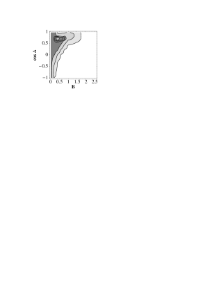
FIG. 2.: Contour plot of the two-dimensional likelihood for $B$ and ${\rm cos}\Delta$. The contours enclose 40%, 86% and 99% of the likelihood and the star marks the peak.

Figure 3 summarizes our results: we plot the one-dimensional likelihood functions obtained by marginalizing all the remaining parameters. Panel a shows that the contribution of isocurvature perturbations can be as large as the adiabatic perturbations, or even larger: we find that $B<1.3$ to 95% c.l.. In contrast, uncorrelated isocurvature perturbations cannot exceed $B<0.5$ to the same c.l.. The likelihood functions for $n$ and $\Omega_{\Lambda}$ extend toward smaller values, as anticipated, while the CDM and the baryon density estimates remain quite unaffected. The average values are $n=0.94\pm 0.1$, $\omega_{b}=0.023\pm 0.004$, $\omega_{c}=0.1\pm 0.03$, $\Omega_{\Lambda}=0.72\pm 0.11$, .

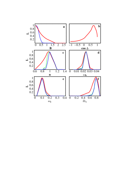
FIG. 3.: One-dimensional likelihood functions in arbitrary units. Green (light) dotted lines for the purely adiabatic models ($B=0$); blue short-dashed lines for uncorrelated fluctuations ($\cos\Delta=0$); red (dark) solid lines for correlated fluctuations. See text for further explanation.

By contrast, Enqvist et al [14] found that a large uncorrelated isocurvature contribution is only consistent with blue tilted slopes. The reason for this difference is that correlations can cause the acoustic peak height to increase relative to the Sachs Wolfe plateau (see Fig. 1) unlike the case of independent perturbations where the relative height always decreases. Trotta et al [16] found that the CMB data was not consistent with a significant CDM isocurvature contribution because they restricted the primordial slope, $n$, to be unity.

As can be seen from Fig. 3 our estimates of $\omega_{b}$ and $\omega_{c}$ are virtually unaffected by the addition of correlated CDM isocurvature perturbations. Thus, in our model, the nature of the isocurvature component can be investigated almost independently of the composition of the matter component.

The main conclusion of the present work is that the current CMB data is consistent with a large correlated CDM isocurvature perturbation contribution when the spectral slopes is allowed a tilt to the red ($n<1$). The higher precision of future satellite data has the potential to detect the isocurvature contribution, if any, thereby showing that inflation was not a single-field process.

The authors are grateful to David Langlois, Roy Maartens and Carlo Ungarelli for useful discussions. CG was supported by the ORS, and DW by the Royal Society.

REFERENCES

- [1] C. B. Netterfield et al., astro-ph/0104460.
- [2] N. W. Halverson et al., astro-ph/0104489.
- [3] A. T. Lee et al., astro-ph/0104459.
- [4] M. Tegmark et al., astro-ph/0008167
- [5] P. de Bernardis et al., astro-ph/0105296; R. Stompor et al., Astrophys. J. 561, L7 (2001); C. Pryke et al., astro-ph/0104490; X. Wang et al., astro-ph/0105091.
- [6] A.D. Linde and L.A. Kofman, Nucl. Phys. B 282 (1987) 555. D. Polarski and A. A. Starobinsky, Phys. Rev. D 50, 6123 (1994). J. García-Bellido and D. Wands, Phys. Rev. D 53 (1996) 5437; A.D. Linde and V. Mukhanov, Phys. Rev. D 56 (1997) 535; M. Sasaki and T. Tanaka, Prog. Theor. Phys. 99, 763 (1998).
- [7] D. Langlois, Phys. Rev. D 59, 123512 (1999).
- [8] C. Gordon et al., Phys. Rev. D 63, 023506 (2001).
- [9] J. Hwang and H. Noh, Phys. Lett. B 495, 277 (2000).
- [10] N. Bartolo et al., Phys. Rev. D 64 (2001) 083514.
- [11] G. Efstathiou and J. R. Bond, Mon. Not. Roy. Astron. Soc. 218, 103 (1986); H. Kodama and M. Sasaki, Int. J. Mod. Phys. A1, 265 (1986); A2, 491 (1987).
- [12] M. Bucher et al., Phys. Rev. D 62, 083508 (2000); M. Bucher et al., astro-ph/0007360; M. Bucher et al., astro-ph/0012141.
- [13] R. Stompor et al., Ap. J. 463 (1996) 8; E. Pierpaoli et al., JHEP 9910, 015 (1999); M. Kawasaki and F. Takahashi, Phys. Lett. B 516 (2001) 388.
- [14] K. Enqvist et al., Phys. Rev. D 62, 103003 (2000).
- [15] D. Langlois and A. Riazuelo, Phys. Rev. D 62, 043504 (2000).
- [16] R. Trotta et al., Phys. Rev. Lett. 87 (2001) 231301.
- [17] D. Wands et al., Phys. Rev. D 62, 043527 (2000).
- [18] J.R. Bond et al., Ap. J., 533, 19 (2000).
- [19] U. Seljak and M. Zaldarriaga, Ap.J., 469, 437 (1996).