Shape Reconstruction and Weak Lensing Measurement with Interferometers: A Shapelet Approach

Abstract

We present a new approach for image reconstruction and weak lensing measurements with interferometers. Based on the shapelet formalism presented in Refregier (2001), object images are decomposed into orthonormal Hermite basis functions. The shapelet coefficients of a collection of sources are simultaneously fit on the $uv$ plane, the Fourier transform of the sky brightness distribution observed by interferometers. The resulting $\chi^{2}$-fit is linear in its parameters and can thus be performed efficiently by simple matrix multiplications. We show how the complex effects of bandwidth smearing, time averaging and non-coplanarity of the array can be easily and fully corrected for in our method. Optimal image reconstruction, co-addition, astrometry, and photometry can all be achieved using weighted sums of the derived coefficients. As an example we consider the observing conditions of the FIRST radio survey (Becker, White & Helfand 1995; White et al. 1997). We find that our method accurately recovers the shapes of simulated images even for the sparse $uv$ sampling of this snapshot survey. Using one of the FIRST pointings, we find our method compares well with CLEAN, the commonly used method for interferometric imaging. Our method has the advantage of being linear in the fit parameters, of fitting all sources simultaneously, and of providing the full covariance matrix of the coefficients, which allows us to quantify the errors and cross-talk in image shapes. It is therefore well-suited for quantitative shape measurements which require high-precision. In particular, we show how our method can be combined with the results of Refregier & Bacon (2001) to provide an accurate measurement of weak lensing from interferometric data.

1 Introduction

Interferometers are widely used for astronomical observations as they provide high angular resolutions and large collecting areas. Existing interferometers in the radio (e.g. the Very Large Array (VLA), the Berkeley-Illinois-Maryland Association (BIMA), etc.) and in the optical band (e.g., the Center for High Angular Resolution Astronomy (CHARA), the Palomar Testbed Interferometer, the Keck Interferometer, the Very Large Telescope (VLT) Interferometer, etc.) will soon be complemented by new facilities such as the Expanded Very Large Array (EVLA), the Square Kilometer Array (SKA), the Atacama Large Millimeter Array (ALMA), and the Low Frequency Array (LOFAR). Interferometers are now also being developed to produce maps of the Cosmic Microwave Background on small scales (e.g., the Cosmic Background Imager (CBI), the Array for Microwave Background Anisotropy (AMiBA), the Very Small Array (VSA), etc).

Interferometric arrays, however, do not provide a direct image of the observed sky, but instead measure its Fourier transform at a finite number of discrete samplings, or ‘$uv$’ points, corresponding to each antenna pair in the array. The image in real space must therefore be reconstructed from the $uv$ plane by inverse Fourier transform while deconvolving the effective beam arising from the finite sampling (see Thompson et al. 1986, Perley et al. 1989, and Taylor et al. 1999 for reviews). For this purpose several elaborate methods have been developed. For instance, the commonly used CLEANing algorithm implemented in the NRAO AIPS software package (Hogbom 1974; Schwarz 1978; Clark 1980; Cornwell 1983), relies on successive subtraction of real-space delta functions from the $uv$ plane. Another method is based on Maximum Entropy (e.g., Cornwell & Evans 1985) and consists of finding the simplest image consistent with the $uv$ data. These methods are well-tested and appropriate for various applications; however, the methods are non-linear and do not necessarily converge in a well-defined manner. Consequently, they are not well-suited for quantitative image shape measurements requiring high precision. In particular, weak gravitational lensing (see Mellier 1999; Bartelmann & Schneider 2000 for reviews) requires the statistical measurements of weak distortions in the shapes of background objects and thus cannot afford the instabilities and potential biases inherent in these methods. While interferometric surveys offer great promises for weak lensing (Kamionkowski et al. 1998; Refregier et al 1998; Schneider 1999), a different approach for shape measurements is therefore required to achieve the necessary accuracy and control of systematics.

In this paper, we present a new method for reconstructing images from interferometric observations. It is based on the formalism introduced by Refregier (2001, Paper I) and Refregier & Bacon (2001, Paper II), in which object shapes are decomposed into orthonormal shape components, or ‘shapelets’. The Hermite basis functions used in this approach have a number of remarkable properties which greatly facilitate the modeling of object shapes. In particular, they are invariant under Fourier transformation (up to a rescaling) and are thus a natural choice for interferometric imaging. We show how shapelet components can be directly fitted on the $uv$ plane to reconstruct an interferometric image. The fit is linear in the shapelet coefficients and can thus be performed by simple matrix multiplications. Since the shapelet components of all sources are fitted simultaneously, cross-talk between different sources (e.g., when the sidelobe from one source falls at the position of a second source) are avoided, or at least quantified. The method also provides the full covariance matrix of the shapelet coefficients, and is robust. We also show how the complex effects of bandwidth smearing, time averaging and non-coplanarity of the array can be easily and fully corrected for in our method. Our method is thus well-suited for applications requiring unbiased, high-precision measurements of object shapes. In particular, we show how the method can be combined with the results of Paper II to provide a clean measurement of weak gravitational lensing with interferometers. We test our methods using both observations from the FIRST radio survey (Becker et al. 1995; White et al. 1997) and numerical simulations corresponding to the observing conditions of that survey. We also show how our method can be implemented on parallel computers and discuss its performance in comparison with the CLEANing method.

Our paper is organized as follows. In §2, we first summarize the relevant features of the shapelet method. In §3, we describe how shapelets can be applied to image reconstruction with interferometers. In §4, we discuss tests of the method using both simulated and real FIRST observations. In §5 we show how our method can be used for weak lensing applications. Our conclusions are summarized in §6.

2 Shapelet Method

We begin by summarizing the relevant components of the shapelet method described in Paper I. In this approach, the surface brightness $f({\mathbf{x}})$ of an object is decomposed as

$$f({\mathbf{x}})=\sum_{{\mathbf{n}}}f_{{\mathbf{n}}}B_{{\mathbf{n}}}({\mathbf{x}};\beta),$$ (1)

where

$$B_{{\mathbf{n}}}({\mathbf{x}};\beta)\equiv\frac{H_{n_{1}}(\beta^{-1}x_{1})~{}H_{n_{2}}(\beta^{-1}x_{2})~{}e^{-\frac{|x|^{2}}{2\beta^{2}}}}{\left[2^{(n_{1}+n_{2})}\pi~{}\beta^{2}~{}n_{1}!~{}n_{2}!\right]^{\frac{1}{2}}}$$ (2)

are the two-dimensional orthonormal Hermite basis functions of characteristic scale $\beta$, $H_{m}(\xi)$ is the Hermite polynomial of order m, ${\mathbf{x}}=(x_{1},x_{2})$ and ${\mathbf{n}}=(n_{1},n_{2})$. The basis is complete and yields fast convergence in the expansion if $\beta$ and $x=0$ are, respectively, close to the size and location of the object. The basis functions can be thought of as perturbations around a two-dimensional Gaussian, and are thus natural bases for describing the shapes of most astronomical objects. They are also the eigenfunctions of the Quantum Harmonic Oscillator (QHO), allowing us to use the powerful formalism developed for that problem. A similar decomposition scheme using Laguerre basis functions has been independently proposed by Bernstein & Jarvis (2001).

The Hermite basis functions have remarkable mathematical properties. In particular, let us consider the Fourier transform of an object intensity, $\tilde{f}({\mathbf{k}})=(2\pi)^{-\frac{1}{2}}\int_{-\infty}^{\infty}d^{2}{x}f({\mathbf{x}})e^{i{\mathbf{k}}\cdot{\mathbf{x}}}$. It can be decomposed as $\tilde{f}({\mathbf{k}})=\sum_{{\mathbf{n}}}f_{{\mathbf{n}}}~{}\widetilde{B}_{{\mathbf{n}}}({\mathbf{k}};\beta)$, where $\widetilde{B}_{{\mathbf{n}}}({\mathbf{k}};\beta)$ are the Fourier-transforms of the basis functions, which obey the dual property

$$\widetilde{B}_{{\mathbf{n}}}({\mathbf{k}};\beta)=i^{(n_{1}+n_{2})}B_{{\mathbf{n}}}({\mathbf{k}};\beta^{-1}).$$ (3)

From the orthonomality of the basis functions, the coefficients are given by

$$f_{{\mathbf{n}}}=\int_{-\infty}^{\infty}~{}d^{2}{k}~{}\tilde{f}({\mathbf{k}})~{}\widetilde{B}_{{\mathbf{n}}}({\mathbf{k}};\beta).$$ (4)

This invariance (up to a rescaling) under Fourier transformation (Eq. [3]) makes this basis set a natural choice for interferometric imaging.

3 Shapelet Reconstruction with Interferometers

In this section, we describe how shapelets can be applied to interferometric imaging. We first briefly discuss how images are mapped onto the $uv$ plane by interferometers. We also show how the $uv$ plane can be binned into cells to reduce computation time and memory requirements. We then describe how the shapelet coefficients can be directly fit onto the binned $uv$ plane using a linear $\chi^{2}$ procedure. Finally, we describe how the resulting shapelet coefficients can be optimally combined to reconstruct the image, to co-add several pointings, and to measure shape parameters.

3.1 Interferometric Observations

An interferometer consists of an array of antennae whose output signals are correlated to measure a complex ‘visibility’ for each antenna pair (see Thompson et al. 1986, Perley et al. 1989, and Taylor et al. 1999 for reviews). Each visibility is then assigned a point on the ‘$uv$ plane’ corresponding to the two-dimensional spacings between the antennae. In practice, the visibilities are close to, but not exactly equal to a two-dimensional Fourier transform of the sky brightness. Within the conventions of Perley, Schwab & Bridle (1989) for the VLA, the visibility measured for the antenna pair $(i,j)$ at time $t$ and at frequency $\nu$ is indeed given by

$$V_{ij}(\nu,t)=\int d^{2}l~{}\frac{A({\mathbf{l}},\nu)f({\mathbf{l}},\nu,t)}{\sqrt{1-|l|^{2}}}e^{-2\pi i[ul+vm+w(\sqrt{1-|l|^{2}}-1)]},$$ (5)

where $f({\mathbf{l}},\nu,t)$ is the surface brightness of the sky at position ${\mathbf{l}}=(l,m)$ with respect to the phase center, and $A({\mathbf{l}},\nu)$ is the (frequency-dependent) primary beam. For the VLA, the primary beam power pattern can be well-approximated as the Bessel function $2J_{1}(z)/z$, where $z\simeq 3.234~{}r\theta_{p}^{-1},~{}\theta_{p}=30^{\prime}.83\times\left(\frac{1.4{\rm GHz}}{\nu}\right)$, $\nu$ is the observation frequency and $r$ is the position offset from the phase center (Condon et al. 1998). The $u,v,w$ coordinates are given by

$$\left(\begin{array}[]{c}u\\ v\\ w\end{array}\right) = \left(\begin{array}[]{ccc}\sin H_{0}&\cos H_{0}&0\\ -\sin\delta_{0}\cos H_{0}&\sin\delta_{0}\sin H_{0}&\cos\delta_{0}\\ \cos\delta_{0}\cos H_{0}&-\cos\delta_{0}\sin H_{0}&\sin\delta_{0}\\ \end{array}\right)$$ (16)

$$\times\left(\begin{array}[]{c}L_{x}\\ L_{y}\\ L_{z}\end{array}\right)\frac{1}{\lambda},$$

where $\lambda=c\nu^{-1}$ is the wavelength of observation, $H_{0}$ and $\delta_{0}$ are the hour angle and declination of the phase center, and $(L_{x},L_{y},L_{z})$ are the coordinate differences for the two antennas. The latter are measured in a fixed-Earth coordinate system, for which the sky rotates about the $\hat{L}_{z}$ axis. Note that the $(u,v,w)$ positions of the visibilities define the synthesized beam pattern. Since the $(u,v,w)$ coordinates are entirely determined by the antenna positions, source coordinates, and time and frequency of the observations, the synthesized beam is precisely known for interforemeters.

Only in the absence of a primary beam ($A=1$), for observations at zenith ($w=0$), and for small displacements from the phase center ($l,m\ll 1$), does the visibility reduce to an exact Fourier Transform of the intensity. Furthermore, the visibilities are measured in practice by averaging over small time and frequency intervals. The resulting averaged visibility is given by

$$\overline{V}_{ij}=\int dt\int d\nu~{}T(t)G(\nu)V_{ij}(t,\nu)$$ (17)

where $T(t)$ and $G(t)$ are the time and frequency window functions, respectively, and are normalized as $\int dtT(t)=\int d\nu G(\nu)\equiv 1$. Because the time and frequency intervals are typically very small, this double integral can be evaluated by Taylor expanding $V_{ij}(t,\nu)$ about the central values $t_{0}$ and $\nu_{0}$ of the window functions. For square-hat window functions of width $\Delta t$ (exact) and $\Delta\nu$ (approximate), respectively, we obtain

$$\overline{V}_{ij} \simeq V_{ij}(t_{0},\nu_{0})+\frac{1}{24}\left[\frac{\partial^{2}V_{ij}(t_{0},\nu_{0})}{\partial t^{2}}(\Delta t)^{2}\right.$$ (18)

$$\left.+\frac{\partial^{2}V_{ij}(t_{0},\nu_{0})}{\partial\nu^{2}}(\Delta\nu)^{2}\right]+\cdots$$

When the telescope points to a fixed location on the sky, the hour angle of the phase center changes as $H_{0}(t)\propto\omega_{E}t$, where $\omega_{E}$ is the angular frequency of the Earth. On the other hand, the declination $\delta_{0}$ of the phase center remains constant.

The above expression for $\overline{V}_{ij}$ can thus be computed analytically, leaving the two-dimensional ${\mathbf{l}}$-integral to evaluate numerically. Note that this provides a direct and complete treatment of primary beam attenuation, time-averaging, bandwidth smearing and non-coplanarity of the array. These effects are difficult to correct for in the context of the standard CLEANing method.

3.2 Binning in the $uv$ plane

In practice, the number of visibilities per observation is large ($>10^{5}$). Directly fitting the shape parameters to all $uv$ points would thus require prohibitively large computing time and memory. Instead, we use a binning scheme to reduce the effective number of $uv$ points without loosing information. In the $uv$ plane, we set a grid of size $\Delta u=\frac{1}{2}~{}{\Delta l}^{-1}$ and average the visibilities inside each cell, where $\Delta l$ is one-half of the intended field of view, and the factor $\frac{1}{2}$ accounts for the Nyquist frequency. The choice of $\Delta u$ is designed both to minimize the number of cells and to avoid smearing at large angular scales, which would otherwise act like an effective primary beam attenuation. We thus calculate the average visibility in the $uv$ cell $c$ (of size $\Delta u$) as

$$\overline{V}_{c}=\frac{1}{N_{c}}\sum_{ij\in c}\overline{V}_{ij}$$ (19)

where $N_{c}$ is the number of visibilities in the cell. This is the data we will use to reconstruct the image.

3.3 Fitting for the shapelet coefficients

We now wish to model the intensity $f_{s}(l,m)$ of each source $s$ as a sum of shapelet basis functions

$$f_{s}({\mathbf{l}})=\sum_{\mathbf{n}}f_{{\mathbf{n}}s}B_{\mathbf{n}}({\mathbf{l}}-{\mathbf{l}}_{s};\beta_{s}),$$ (20)

centered on the source centroid ${\mathbf{l}}_{s}=(l_{s},m_{s})$, and scale $\beta_{s}$. Our goal is to estimate the shapelet coefficients $f_{{\mathbf{n}}s}$ of the sources given the binned $uv$ data $\{\overline{V}_{c}\}$. (We will describe how the centroid and shapelet scales are chosen in practice in §4.1). In principle, the full $uv$ plane provides complete shape information for the sources. However, due to the finite number and non-uniform spacings of the antennae, the $uv$ (Fourier) space is poorly sampled, thus hampering the decomposition. This prevents us from performing a simple linear decomposition as is done with optical images in real space (see Paper I). This problem can be largely resolved by making a linear fit to the $uv$ plane with the shapelet coefficients as the free parameters.

For this purpose, the first step is to compute the binned visibilities $\overline{V}_{c}^{{\mathbf{n}}s}$ corresponding to each shapelet basis functions $B_{{\mathbf{n}}s}({\mathbf{l}}-{\mathbf{l}}_{s};\beta_{s})$ for each source $s$. This can be done by first computing the time- and frequency-averaged visibility $\overline{V}_{ij}^{{\mathbf{n}}s}$ by setting $f({\mathbf{l}})=B_{{\mathbf{n}}s}({\mathbf{l}}-{\mathbf{l}}_{s};\beta_{s})$ in Equations (5) and (17). To prevent potential biases introduced by the binning scheme, we evaluate the basis functions at every visibility point and then average them inside each cell to compute $\overline{V}_{c}^{{\mathbf{n}}s}$ just as in Equation (19). Note that this ensures that the systematic distortions induced by the primary beam, bandwidth smearing, time-averaging and non-coplanarity can all be fully corrected in our method.

The next step is to form and minimize

$${\chi}^{2}=({\mathbf{d}}-{\mathbf{M}~{}f})^{T}~{}{\mathbf{C}}^{-1}~{}({\mathbf{d}}-{\mathbf{M}~{}f}),$$ (21)

where ${\mathbf{d}}=\{\overline{V}_{c}\}$ is the data vector, ${\mathbf{M}}=\{\overline{V}_{c}^{{\mathbf{n}}s}\}$ is the theory matrix, and ${\mathbf{f}}=\{f_{{\mathbf{n}}s}\}$ is the parameter vector. The covariance error matrix

$${\mathbf{C}}={\rm cov}[{\mathbf{d}},{\mathbf{d}}]=\left\langle({\mathbf{d}}-\langle{\mathbf{d}}\rangle)^{T}{(\mathbf{d}}-\langle{\mathbf{d}}\rangle)\right\rangle$$ (22)

for the binned visibilities can be estimated in practice either from the distribution of the visibilities in each bin or from the error tables provided by the interferometric hardware.

Because the model is linear in the fitting parameters, the best-fit parameters $\widehat{\mathbf{f}}$ can be computed analytically as (e.g., Lupton 1993)

$$\widehat{\mathbf{f}}=({\mathbf{M}}^{T}{\mathbf{C}}^{-1}{\mathbf{M}})^{-1}{\mathbf{M}}^{T}{\mathbf{C}}^{-1}{\mathbf{d}}.$$ (23)

The covariance error matrix ${\mathbf{W}}={\rm cov}[\widehat{\mathbf{f}},\widehat{\mathbf{f}}]$ of the best-fit parameters is given by

$${\mathbf{W}}=({\mathbf{M}}^{T}{\mathbf{C}}^{-1}{\mathbf{M}})^{-1}$$ (24)

This provides us with an estimate for the shapelet coefficients for each source and for their full covariance matrix. Note that all sources are fitted simultaneously thus avoiding (or at least quantifying) potential cross-talk between different sources (e.g., when a sidelobe from one source falls at the position of a second source). The coefficient covariance matrix can also be used to determine degeneracies produce by the finite $uv$ sampling of the array.

3.4 Combining the Shapelet Coefficients

Now that we have derived estimates $\widehat{f}_{\mathbf{n}}$ for the shapelet coefficients $f_{\mathbf{n}}$ for each source in a pointing, we can combine them to construct an image and to compute useful quantities such as the fluxes, centroids and sizes of the sources.

We first consider the practical problem of co-adding several pointings to derive an optimal image of a source. Let $\widehat{f}_{{\mathbf{n}}p}$ be the coefficients of a source derived from pointing $p$, and let $W_{{\mathbf{n}m}p}$ be the associated covariance error matrix (from Eq. (24)). It is easy to see that the error in the co-added coefficients $\widehat{f}_{\mathbf{n}}$ will be minimized if they are given by the weighted sum

$$\widehat{f}_{\mathbf{n}}=\frac{\sum_{p}W_{{\mathbf{n}}\mathbf{n}p}^{-1}\widehat{f}_{{\mathbf{n}}p}}{\sum_{p}W_{{\mathbf{n}}{\mathbf{n}}p}^{-1}}.$$ (25)

The covariance error matrix $W_{{\mathbf{n}}\mathbf{m}}={\rm cov}[\widehat{f}_{\mathbf{n}},\widehat{f}_{\mathbf{m}}]$ of the co-added coefficients are then given by

$$W_{{\mathbf{n}}{\mathbf{m}}}=\frac{\sum_{p}W_{{\mathbf{n}}{\mathbf{n}}p}^{-1}W_{{\mathbf{n}}{\mathbf{m}}p}W_{{\mathbf{m}}{\mathbf{m}}p}^{-1}}{\left(\sum_{p}W_{{\mathbf{n}}{\mathbf{n}}p}^{-1}\right)\left(\sum_{p}W_{{\mathbf{m}}{\mathbf{m}}p}^{-1}\right)}.$$ (26)

We can then find an optimal weighting to reconstruct the image of a source from the estimated coefficients $\widehat{f}_{\mathbf{n}}$. To do so we seek the reconstructed coefficients given by

$$f^{r}_{\mathbf{n}}=\phi_{\mathbf{n}}\widehat{f}_{\mathbf{n}}.$$ (27)

The weights $\phi_{\mathbf{n}}$ are chosen so that the reconstructed image $f^{r}({\mathbf{l}})=\sum_{\mathbf{n}}f^{r}_{\mathbf{n}}B_{\mathbf{n}}({\mathbf{l}})$ is ‘as close as possible’ to the true image $f({\mathbf{l}})$, in the sense that the least-square difference

$$\int d^{2}l~{}\left[f^{r}({\mathbf{l}})-f({\mathbf{l}})\right]^{2}=\sum_{\mathbf{n}}[f^{r}_{\mathbf{n}}-f_{\mathbf{n}}]^{2}$$ (28)

is minimized. It is easy to show that this will be the case when

$$\phi_{\mathbf{n}}=\frac{|f_{\mathbf{n}}|^{2}}{|f_{\mathbf{n}}|^{2}+W_{{\mathbf{n}}{\mathbf{n}}}}\approx\frac{|\widehat{f}_{\mathbf{n}}|^{2}-W_{{\mathbf{n}}{\mathbf{n}}}}{|\widehat{f}_{\mathbf{n}}|^{2}},$$ (29)

where the right-hand side provides an approximation which can be directly derived from the data. This weighting amounts to Wiener filtering in Shapelet space, in analogy with that performed in Fourier Space (see, e.g., Press et al. 1987). Figures 1 and 2 show several reconstructed images using this weighting scheme. Note that this produces an estimate for the deconvolved image of the source. For display purposes, it is sometimes useful to smooth the reconstructed image by a Gaussian kernel (the ’restoring beam’ in radio parlance). This can easily be done in shapelet space by multiplying the coefficients by the analytic smoothing matrix described in Paper I.

While Wiener filtering yields an optimal image reconstruction, it is not to be used to measure source parameters such as flux, centroid, size, etc. Instead, an unbiased estimator for shape parameters can be derived directly from the shapelet coefficients (see Paper I). For instance, an estimate for the flux $F\equiv\int d^{2}lf({\mathbf{l}})$ of a source is given by $\widehat{F}={\mathbf{A}}^{T}\widehat{\mathbf{f}}$ where

$$A_{n_{1}n_{2}}=\pi^{\frac{1}{2}}\beta 2^{\frac{1}{2}(2-n_{1}-n_{2})}\left(\begin{array}[]{c}n_{1}\\ n_{1}/2\end{array}\right)^{\frac{1}{2}}\left(\begin{array}[]{c}n_{2}\\ n_{2}/2\end{array}\right)^{\frac{1}{2}},$$ (30)

if $n_{1}$ and $n_{2}$ are both even (and vanishes otherwise). The variance uncertainty in the flux is then simply

$$\sigma^{2}[\widehat{F}]={\mathbf{A}}^{T}{\mathbf{W}}{\mathbf{A}},$$ (31)

which provides a robust estimate of the signal-to-noise SNR$=\widehat{F}/\sigma[\widehat{F}]$ of the source. Similar expressions can be used to compute the centroid and rms size of the source. This can be easily generalized to compute in addition the major and minor axes of the source and its position angle. Note that these expressions are, again, estimates for deconvolved quantities.

4 Test of the Method

As an application, we consider the FIRST radio survey (Becker et al. 1995; White et al. 1997), being conducted with the VLA at 1.4 GHz in the B configuration. For this survey, the primary beam FWHM is $\sim$ 30^′ and the angular resolution is $5^{\prime\prime}.4$ (FWHM). The survey currently contains about $7.2\times 10^{5}$ sources with a $5\sigma$ flux-density limit of 1.0 mJy over $A\simeq 8,000$ deg²; the mean source redshift is $\langle z\rangle\sim 1$. Observing time has been allocated to extend its coverage to 9,000 deg². The survey is composed of 165-second ‘grid-pointings’ with a time-averaging interval $\Delta t=5$ seconds. It was conducted in the spectral synthesis mode, with a channel bandwidth of $\Delta\nu=$ 3 MHz. Because this wide-field survey was performed in the snapshot mode, its $uv$ sampling is very sparse. This makes shape reconstruction particularly challenging for FIRST, providing a good test for our method.

As explained in §3.1, higher order effects such as bandwidth smearing and time-averaging produce small distortions in the reconstructed image shapes if they are left uncounted for. These must be carefully corrected for high-precision statistical measurements of object shapes such as those required in weak lensing surveys. The effects are, however, very small and not noticeable on an object-by-object basis. For the purpose of this test, we thus ignore these effects and instead focus on the dominant factor in shape reconstruction, the finite and discrete $uv$ sampling.

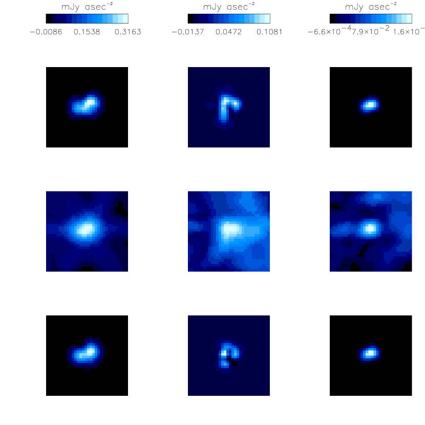
Figure 1: Three sources from the simulation of a FIRST grid pointing. The input images (before the addition of noise), dirty images, and shapelet reconstructions are shown from top to bottom, respectively. The images are 32^′′ across with a 1^′′ pixel size, and the resolution is $\sim$ 5^′′.4 (FWHM). The input source flux densities are (16.0, 4.3, 3.7) mJy from left to right, and the recovered shapelet flux densities calculated using Equation (30) are (16.1, 4.1, 3.8) mJy, respectively, where (10, 21, 6) shapelet coefficients were used in the reconstruction. The noise level in the simulation is about 0.3 mJy beam^-1.

4.1 Simulations

As a first test, we generated simulated VLA data using the observational parameters of FIRST. A grid pointing was generated at zenith with 33 5-second time-averaging intervals and 14 3-MHz channels in the B configuration. Simulated sources were randomly distributed within 23^′.5 of the phase center, the cutoff adopted for creating the final co-added FIRST maps (Becker et al. 1995); the number density, flux density and size distributions chosen for the sources were similar to sources in the FIRST catalog. After generating the visibilities, we added uncorrelated Gaussian noise to the real and imaginary component of each $uv$ data point, with an rms of $\sigma_{v}=\sigma_{n}N_{\rm vis}^{0.5}$, where $N_{\rm vis}$ is the total number of visibilities. The real-space rms noise $\sigma_{n}$ was set to $0.3$ mJy beam^-1, which is somewhat higher than the typical FIRST noise level, $\sim$ 0.2 mJy beam^-1.

We then simultaneously fitted all 23 sources in the grid pointing directly in the $uv$ plane. We imposed the constraint that that source intensities are real (i.e., non-imaginary). Each source $s$ was modeled as a shapelet with scale $\beta_{s}$, maximum shapelet order $n_{{\rm max},s}$, and center position ${\mathbf{l}}_{s}$. In principle, it is possible to determine these parameters with a source detection algorithm which directly uses shapelets. One can, for instance, tile ground-state shapelets with different sizes in the $uv$ plane, and thus detect sources with different sizes. However, this is computationally expensive and, since the FIRST catalog is conveniently available, we have not implemented this algorithm.

Instead, good choices for these parameters were derived from the FIRST catalog, which lists basic shape parameters for each source, such as its centroid, flux density, major and minor axes, and position angle, all obtained from an elliptical Gaussian fit. The shapelet position ${\mathbf{l}}_{s}$ was simply set to the centroid position from the catalog. The choices for the shapelet scales $\beta_{s}$ and maximum shapelet orders $n_{{\rm max},s}$ were derived as follows. As described in Paper I, the Hermite basis functions have two natural scales: $\theta_{\rm max}$ corresponding to the overall extent of the basis functions, and $\theta_{\rm min}$ corresponding to the smallest-scale oscillations in the basis functions. These scales are related to the shapelet scale and maximum order by $\theta_{\rm max}\sim\beta(n_{\rm max}+1)$ and $\theta_{\rm min}\sim\beta(n_{\rm max}+1)^{-1}$. As $n_{\rm max}$ increases, the large-scale size of the shapelet grows, while its small-scale features become finer. The shapelet thus becomes more extended both in real and in Fourier space. We therefore choose $\theta_{\rm max}$ to be the rms major axis from the FIRST catalog, and $\theta_{\rm min}$ to correspond to the longest baseline of the VLA: $\sim$ 1^′′.8 (rms) in real space. This provides us with a choice for $\beta\simeq(\theta_{\rm max}~{}\theta_{\rm min})^{0.5}$ and for $n_{\rm max}\simeq\frac{\theta_{\rm max}}{\theta_{\rm min}}-1$ for each source.

Solving Equation (21), we then obtain the shapelet coefficients and the covariance matrix using Equations (23) and (24). The results are presented in Fig. 1, where the input images (before the addition of noise), inverse Fourier-transformed $uv$ data (‘dirty’ images), and shapelet-reconstructed images (with Weiner filtering, see §3.4) of three of the sources are shown. Each image shown is 32^′′ across and the resolution is about 5^′′.4 (FWHM). The poor $uv$ sampling of FIRST and the effect of noise are evident in the dirty images. For both resolved (left panels) and unresolved or marginally resolved (right panels) sources, the reconstructions agree with the inputs very well. The more complicated structure in the central panel is not fully recovered by shapelets. This is expected, since the small-scale structure of the source is not resolved and therefore can not be fully recovered in the reconstruction.

The comparison between the input and shapelet-reconstructed flux density for all sources in the grid pointing is shown in Figure 4.1. The shapelet flux density is given by Equation (30) and its 1$\sigma$ error by Equation (31). The source flux densities are well-recovered by the shapelets in an unbiased manner. Note the range of error bars at a given input flux is due to the range of source sizes. For instance, for an input flux density of about 2 mJy, the source with a relatively large error bar has a major axis of about $8^{\prime\prime}$ (FWHM), while those with small error bars are unresolved or barely resolved (major axis FWHM $<5^{\prime\prime}$). In general, we find the shapelet reconstruction from the sparsely sampled and noisy simulated data to be in good agreement with the input (noise-free) image. Note that our method can be used to identify and discard spurious sources arising from sidelobes and other artifacts in the dirty image. Indeed, when we place an extra shapelet centered at a random positions in the field, the coefficients of that shapelet are consistent with zero.

Flux density comparison for the simulations: the input flux densities of the 23 sources in the simulated pointing are compared with the shapelet reconstructed flux densities. The solid line corresponds to a perfect reconstruction– i.e., to a recovered flux density equal to the input flux density.

4.2 Data

Next, we test our method by applying it to one of the FIRST grid pointings (14195+38531). For this purpose, we selected all sources within 23^′.5 of the phase center from the FIRST catalog with a measured flux density limit (i.e., including the primary beam response) of 0.75 mJy. For each of the resulting 23 sources, we use the source major axis to estimate $\beta$ and $n_{\rm max}$ as described in the previous section. We then simultaneously fit all the sources for the shapelet coefficients directly in the $uv$ plane. Note that the shapelet coefficients obtained are deconvolved coefficients.

Figure 2 shows the reconstruction of three representative sources in the bottom panels. Also shown for comparison are the images of the sources constructed using the standard AIPS CLEAN algorithm with a CLEANing limit of 0.5 mJy (central panel), along with the dirty images (top panel). Each panel is 32^′′ across and the FWHM of the FIRST resolution is 5^′′.4. The shapelet method does not involve image pixels in the modeling; one is therefore free to specify the pixel size when constructing the images. Here the dirty and CLEANed images have pixel sizes of 1^′′.8, while the shapelet images have pixel sizes of 1^′′ and thus show finer details. For demonstration, the shapelet reconstructions have been Weiner-filtered using the resulting covariance matrix. For a direct comparison, they have also been smoothed with a Gaussian kernel with a standard deviation of 2^′′.3, reproducing the ’restoring beam’ of the CLEANed image. We find that the shapelet reconstructions compare well with the CLEANed images.

In further tests, we have encountered cases where a bright source ($>100$ mJy) lies in or near a grid pointing. We have found that the presence of the bright source does not affect the fit of the other sources in the grid in a noticeable way. Our method can thus well handle the dynamical range of the FIRST survey, which spans more than 3-orders of magnitude. For fainter sources ($<1$ mJy; i.e., detection SNR $<6$), the reconstructions are rather poor at times, in contrast to those for brighter sources (which are almost always well fitted). This is of course reasonable, given the larger impact of noise for faint sources.

In Figure 5 we display a portion of the covariance matrix for the shapelet coefficients for the nine sources in the pointing with the highest peak flux densities. The horizontal and vertical lines separate the nine sources. The diagonal line from the lower-left to the upper-right corner represents the variance of the shapelet coefficients. The block-diagonal boxes are the covariance matrix of the coefficients of the nine sources. The off-diagonal blocks quantify the cross-talk between sources. Note that the correlation between coefficients are roughly an order of magnitude smaller than the variance. Figure 5 shows the error in the shapelet coefficients (n1,n2) of the source shown in the left panels of Figure 2. (These errors are the diagonal segment of the 4^th diagonal box counting from the lower left in Fig. 5). In general, we find that higher-$n$ coefficients tend to be noisier. This is expected since convolution (or, equivalently, $uv$ sampling) suppresses the small scale information encoded by coefficients with large $n$ (see paper I). The covariance matrix thus provides us with useful information on the error in each coefficient, and quantifies cross-talk between coefficients both within and among sources.

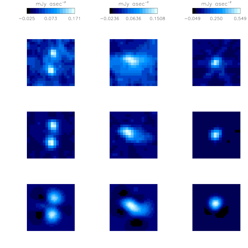
Figure 2: Three sources from one of the FIRST grid pointings. The dirty images, CLEAN images, and shapelet reconstructions are shown from top to bottom, respectively. The images are 32^′′ across and the resolution is about 5^′′.4 (FWHM). The dirty and CLEAN images are displayed with a 1^′′.8 pixel size, while the shapelet reconstruction images have 1^′′ pixels. The source flux densities measured by integrating fitted elliptical Gaussians to CLEANed sources are (13.4, 14.2, 19.5) mJy, from left to right, and the recovered shapelet flux densities calculated using Eq. (30) are (17.0, 13.8, 22.5) mJy, respectively. We used (15, 28, 6) shapelet coefficients in the reconstructions, along with Wiener filtering and smoothing by a Gaussian restoring beam with a standard deviation of 2.3^′′.

4.3 Computation

Since the shapelet coefficients of all sources are simultaneously fit to a large number of visibilities, the computing memory required for the calculation is not negligible. We have implemented the method on the UK COSMOS SGI Origin 2000 supercomputer, which has 64 R10000 MIPS processors with a shared-memory structure. Numerically, the shapelet coefficients can be obtained by performing simple matrix operations as in Equation (23), or by solving the linear least-squares problem, ${\mathbf{M}~{}f}={\mathbf{d}}$, using matrix factorization or singular value decomposition, and assuming that the data covariance matrix ${\mathbf{C}}$ is diagonal. Both methods can be efficiently parallelized. With our binning scheme, the run-time memory required for this particular FIRST grid pointing was about 700 MB, for 23 sources and a total of 177 shapelet parameters. The CPU time required was about 26 seconds with 10 processors or about 5 minutes in scalar mode. For other grid pointings with different numbers of sources, the computation time ranges between 20 and 60 seconds with 10 processors, with a run time memory between 0.5 to 1.5 GB.

5 Applications to Weak Lensing

Weak gravitational lensing is now established as a powerful method for mapping the distribution of the total mass in the Universe (for reviews see Mellier 1999; Bartelmann & Schneider 2000). This technique is now routinely used to study the dark matter distribution of galaxy clusters and has recently been detected in the field (Wittman et al 2000; van Waerbeke et al 2000; Bacon, Refregier & Ellis 2000; Kaiser et al 2000; Maoli et al 2001; Rhodes, Refregier & Groth 2001; van Waerbeke et al 2001). All studies of weak lensing have been performed in the optical and IR bands, where the images are directly obtained in real space.

The covariance matrix for the shapelet coefficients of nine sources in the FIRST grid pointing. The sources are separated by the horizontal and vertical lines. The diagonal entries correspond to the variance (i.e., error) of each shapelet coefficient. The block-diagonal boxes are the covariance matrix of the coefficients for each of the nine sources. The off-diagonal boxes quantify the cross-talk between sources.

The error matrix for one of the FIRST sources plotted in the (n1, n2) plane. The shapelet reconstructed image of this source is shown on the bottom-left panel of Fig.2. These variances can also be used to Weiner filter the coefficients for image reconstruction, as described in §3.4.

There are a number of reasons to try to extend these studies to interferometric images in the radio band. Firstly, the brightest radio sources are at high redshift, thereby increasing the strength of the lensing signal. Secondly, radio interferometers have a well-known and deterministic convolution beam, and thus do not suffer from the irreproducible effects of atmospheric seeing. Thirdly, existing surveys such as the FIRST radio survey (Becker et al. 1995; White el al. 1997) provide a sparsely sampled but very wide-area survey, which offers the unique opportunity to measure a weak lensing signal on large angular scales (Kamionkowski et al. 1998; Refregier et al. 1998; see also Schneider (1999) for the case of SKA). Finally, surveys at higher frequencies or in more extended antenna configurations could potentially yield very high angular resolution and are not limited by the irreducible effects of the seeing disk in ground-based optical surveys.

Because the distortions induced by lensing are only on the order of 1%, the shapes of background objects must be measured with high precision. In addition, systematic effects such as the convolution beam and instrumental distortions must be tightly controlled. For this purpose, a number of shear measurement methods have been developed. The original method of Kaiser, Squires & Broadhurst (1995) was found to be acceptable for current cluster and large-scale structure surveys (Bacon et al. 2000b; Erben et al. 2000), but are not sufficiently reliable for future high-precision surveys. Consequently, several other methods have been proposed (Kuijken 1999; Kaiser 2000; Rhodes, Refregier & Groth 2000, Berstein & Jarvis 2001).

Recently, Refregier & Bacon (2001, Paper II) developed a new method based on shapelets and demonstrated its simplicity and accuracy for ground-based surveys. It is thus straightforward to apply this method to interferometric measurements. Indeed, the shapelet coefficients $f_{\mathbf{n}}$ which we derive from the fit on the $uv$ plane (after co-adding if required) are already deconvolved from the effective beam and can thus be directly used to estimate the shear. This can be done using the estimators for the shear components $\gamma_{1}$ and $\gamma_{2}$ which are given by (see Paper II)

$$\gamma_{i}=\frac{f_{\mathbf{n}}-\langle f_{\mathbf{n}}\rangle}{\sum_{\mathbf{m}}\hat{S}_{i{\mathbf{n}}{\mathbf{m}}}\langle f_{\mathbf{m}}\rangle},$$ (32)

where the sum is over even (odd) shapelet coefficients for $\gamma_{1}$ ($\gamma_{2}$) and the brackets denote an average over an (unlensed) object ensemble. The matrix $\hat{S}_{i{\mathbf{n}}{\mathbf{m}}}$ is the shear matrix, and can be expressed as simple combinations of ladder operators in the QHO formalism. These estimators for individual shapelet components are then optimally weighted and combined to provide a minimum-variance estimator for the shear. This permits us to achieve the highest possible sensitivity (while remaining linear in the surface brightness) by using all the available shape information of the lensed sources.

In Kamionkowski et al. (1998) and Refregier et al. (1998), it has been shown that the FIRST radio survey is a unique database for measuring weak lensing by large-scale structure on large angular scales. In a future paper, we will apply the method described here to this survey, search for the lensing signal, and, from its amplitude, derive constraints on cosmological parameters.

6 Conclusions

We have presented a new method for image reconstruction from interferometers. Our method is based on shapelet decomposition and is simple and robust. It consists of a linear fit of the shapelet coefficients directly in the $uv$ plane, and thus permits a full correction of systematic shape distortions caused by bandwidth smearing, time-averaging and non-coplanarity. Because the fit is linear in the shapelet coefficients it can be implemented as simple matrix multiplications. It provides the full covariance matrix of the shapelet coefficients which can then be used to estimate errors and cross-talk in the recovered shapes of sources. We have shown how source shapes from different pointings can be easily co-added using a weighted sum of the recovered shapelet coefficients. We have also described how the shapelet parameters could be combined to derive optimal image reconstruction, photometry, astrometry and pointing co-addition.

Our method can be efficiently implemented on parallel computers. We find that a fit to all the sources in a FIRST grid pointing takes about 1 minute on an Origin 2000 supercomputer with 10 processors (10 minutes in scalar mode). Because we are fitting all sources simultaneously, 0.5 to 1.5 GB of memory is required.

To test our methods, we considered the observing conditions of the FIRST radio survey (Becker et al. 1995; White et al. 1997) whose snapshot mode yields a sparse sampling in $uv$ space. Using numerical simulations tuned to reproduce the conditions of FIRST, we find that the sources are well-reconstructed with our method. We have also applied our method to a FIRST snapshot pointing and found that the shapes are well-recovered. The reconstruction of our method compares well with the CLEAN reconstruction, without suffering the potential biases inherent in the latter method. Our method is thus well-suited for applications requiring quantitative and high-precision shape measurements.

In particular, our method is ideal for the measurement of the small distortions induced by gravitational lensing in the shape of background sources by intervening structures. Such a measurement from CLEANed images may well not be practical since the systematic distortions induced by that method are very difficult to control. (One could perhaps imagine running numerical simulations to calibrate the shear estimator, but this would be both computationally expensive and rather uncertain). We have shown how our results can be combined with the shear measurement method described in Refregier & Bacon (2001) to derive a measurement of weak lensing with interferometers. This is facilitated both by the fact that our recovered shapelet coefficients are already deconvolved from the effective (dirty) beam, and as a consequence of the remarkable properties of shapelets under shears.

Our method therefore opens the possibility of high-precision measurements of weak lensing with interferometers. While to date all weak-lensing studies have been carried using optical data (and therefore in real space), an interferometric measurement of weak lensing in the radio band is very attractive (Kamionkowski et al. 1998; Refregier et al. 1998; Schneider 1999). Indeed, the lensing signal is expected to be larger because radio sources have a higher mean redshift. In addition, such a measurement would not suffer from the irreproducible effects of atmospheric seeing. Instead, the effective (dirty) beam is fully known for interferometers and the noise properties of the antennas are well-understood. As a result, the impact of systematic effects, the crucial limitation in the search for weak lensing, are expected to be lower with radio interferometers. In a future paper, we will describe our measurement of weak lensing by large-scale structure with the FIRST survey using the present method.

References

- (1) Bacon, D., Refregier, A., Ellis, R., 2000, MNRAS, 318, 625
- (2) Bacon, D. Refregier, A., Clowe, D., & Ellis, R., 2000b, to appear in MNRAS, preprint astro-ph/0007023
- (3) Bartelmann, M., & Schneider, P., 2000, preprint astro-ph/0007023
- (4) Becker, R.H., White, R.L., Helfand, D.J., 1995, ApJ, 450, 559
- (5) Bernstein, G.M., & Jarvis, M., 2001, accepted by AJ, astro-ph/0107431
- (6) Clark, B.G., 1980, A&A, 89, 377
- (7) Condon,J.J., Cotton,W.D., Greisen, E.W., Yin, Q.F., Perley, R.A., Taylor, G.B., Broderick, J.J., 1998, AJ, 115, 1695
- (8) Cornwell, T,J., 1983, A&A, 121, 281
- (9) Cornwell, T.J. & Evans, K.F., 1985, A&A, 143, 77
- (10) Erben T., van Waerbeke, L., Bertin, E., Mellier, Y., Schneider, P., 2001, A&A, 366, 717
- (11) Hogbom, J.,A., 1974, A&AS, 15, 417
- (12) Kaiser, N., 2000, ApJ, 537, 555
- (13) Kaiser, N., Wilson, G., Luppino, G. A., 2000, preprint astro-ph/0003338
- (14) Kamionkowski, M., Babul, A., Cress, C., Refregier, A., 1998, MNRAS, 301, 1064
- (15) Kuijken, K., 1999, A&A, 352, 355
- (16) Lupton, R., 1993, Statistics in Theory and Practice, Princeton University Press
- (17) Maoli, R. et al, 2001, A&A, 368, 766
- (18) Mellier, Y., 1999, ARA&A, 37, 127
- (19) Narayan, R., & Bartelmann, M., 1999, in Formation of Structure in the Universe. Ed. by Dekel, A. and Ostriker, J.P., p.360 (preprint astro-ph/9606001)
- (20) Perley, R.A., Schwab, F.R., & Bridle, A.H., 1989, Synthesis Imaging in Radio Astronomy, A.S.P.C.S. Vol. 6
- (21) Press, W.H., Teukolsky, S.A., Vetterling, W.T., Flannery, B.P., 1987, Numerical Recipes, Cambridge University Press
- (22) Refregier et al. 1998, in Proc. of the XIVth IAP meeting, Wide-Field Surveys in Cosmology, held in Paris in May 1998, eds. Mellier, Y. & Colombi, S. (Paris: Frontieres), preprint astro-ph/9810025
- (23) Refregier, A., 2001, (Paper I) submitted to MNRAS, preprint astro-ph/0105178
- (24) Refregier, A. & Bacon, D.J., 2001, (Paper II) submitted to MNRAS, preprint astro-ph/0105179
- (25) Rhodes, J., Refregier, A., & Groth, E., 2000, ApJ, 536, 79
- (26) Rhodes, J., Refregier, A., & Groth, E., 2001, to appear in ApJL, preprint astro-ph/0101213
- (27) Schneider, P., 1999, in Perspectives on Radio Astronomy, Scientific Imperatives at cm and m wavelengths, Proceedings of a workshop in Amsterdam, April 1999, preprint astro-ph/9907146
- (28) Schwarz, U.J., 1978, A&A, 65, 345
- (29) Taylor, G.B., Carilli, C.L., & Perley, R.A., 1999, Synthesis Imaging in Radio Astronomy II, A.S.P.C.S. Vol. 180
- (30) Thompson, A.R., Moran, J. & Swenson, JR., G.W, 1986, Interferometry and Synthesis in Radio Astronomy (Wiley-Interscience)
- (31) van Waerbeke, L. et al, 2000, A&A, 358, 30.
- (32) van Waerbeke, L. et al, 2001, submitted to A&A, preprint astroph/0101511.
- (33) White, R.L., Becker, R.H., Helfand, D.J., Gregg, M.D., 1997, ApJ, 475, 479
- (34) Wittman, D., Tyson, J. A., Kirkman, D., Dell’Antonio, I., Bernstein, G., 2000, Nature, 405, 143.