A Multi-Threaded Fast Convolver for Dynamically Parallel Image Filtering

Abstract

2D convolution is a staple of digital image processing. The advent of large format imagers makes it possible to literally “pave” with silicon the focal plane of an optical sensor, which results in very large images that can require a significant amount computation to process. Filtering of large images via 2D convolutions is often complicated by a variety of effects (e.g., non-uniformities found in wide field of view instruments). This paper describes a fast (FFT based) method for convolving images, which is also well suited to very large images. A parallel version of the method is implemented using a multi-threaded approach, which allows more efficient load balancing and a simpler software architecture. The method has been implemented within in a high level interpreted language (IDL), while also exploiting open standards vector libraries (VSIPL) and open standards parallel directives (OpenMP). The parallel approach and software architecture are generally applicable to a variety of algorithms and has the advantage of enabling users to obtain the convenience of an easy operating environment while also delivering high performance using a fully portable code.

1 Introduction

The ability to process ever larger images at ever increasing rates is a key enabling technology for a wide variety of medical, scientific, industrial and government applications (e.g., next generation MRI/x-ray, environmental monitoring, real-time digital video, surveillance and tracking). Image filtering via 2D convolutions is often the dominant image processing operation in terms of computation cost. Found in almost image processing pipelines 2D convolution is essential for background compensation, image enhancement, smoothing, detection and estimation. In real-time imaging sensors rapid frame rates require very low latency processing, which requires high performance 2D convolutions. In archival image database queries, the size of the image can be enormous and high performance convolutions are necessary in order to complete the query in a reasonable amount of time.

Traditionally, custom chips or coprocessors have been used to alleviate image processing performance bottlenecks. However, as image processing applications become more complex and more software focused (i.e. workstation based) these solutions become less feasible. There are essentially three ways of improving performance in a software centered image processing environment: better algorithms, better optimization and parallel processing. This work applies all three of these approaches specifically to improve the 2D convolution operation. Although the primary aim of this paper is to demonstrate a faster 2D convolution algorithm, a secondary goal is to consider the system issues necessary to effectively integrate this type of technology into readily available image processing environments with minimal software maintenance overhead.

Section two of this paper presents a general FFT based algorithm for implementing 2D convolutions, which is also well suited for wide field of view images. Section three describes a parallel scheme for the convolution algorithm and provides general analyses the computation, communication, and load balancing costs. Section four, discusses a general purpose software architecture for implementing the algorithm and transparently integrating it within high level image processing environments. Section five presents the parallel performance results. Section six gives the conclusions.

2 2D Filtering Algorithm

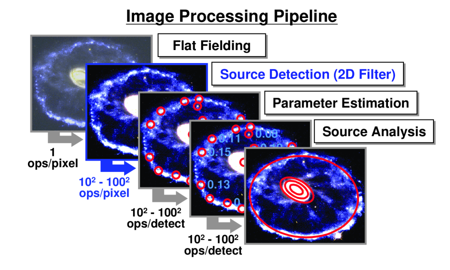
Figure 1: Generic Image Processing Pipeline. Most pipelines consist of steps similar to the above. In this process 2D filtering is the most compute intensive step. Later steps are more complex (e.g. source analysis) but operate on a reduced amount of data. [Cartwheel Galaxy image courtesy of Kirk Borne (ST ScI), and NASA.]

Wide area 2D convolution is a staple of digital image processing. Figure 1 shows one example of how convolution fits into an image processing pipeline. Typically, an image $I(x,y)$ is acquired by a sensor or extracted from an archive. We wish to convolve or filter this image using a kernel $K(x,y)$ to produce a filtered image $F(x,y)$. Mathematically this is equivalent to

$$F(x,y)=\int\int K(x^{\prime},y^{\prime})I(x-x^{\prime},y-y^{\prime})dx^{\prime}dy^{\prime}$$ (1)

For convenience it is reasonable to assume the image and the kernel are $M$ x $M$ and $N$ x $N$ squares, respectively (this condition can be relaxed later without loss of generality). In the discrete case, the above convolution can be computed by the double sum

$$F(i,j)=\sum_{i^{\prime}=0}^{N-1}\sum_{j^{\prime}=0}^{N-1}K(i^{\prime},j^{\prime})I(i-i^{\prime},j-j^{\prime})~{},$$ (2)

where $i$ and $j$ are pixel indices. The above direct summation involves $O(N^{2})$ operations per pixel, which can become prohibitive for large kernels.

2.1 Basic FFT based algorithm

A more efficient implementation of 2D filtering is obtained using the Fast Fourier Transform. This classic result exploits the fact that convolution is equivalent to multiplication in the Fourier domain

$${\hat{F}}({\vec{k}})={\hat{K}}({\vec{k}})\cdot{\hat{I}}({\vec{k}})$$ (3)

where ${\hat{I}}$, ${\hat{K}}$ and ${\hat{F}}$ are the Fourier Transforms

$${\hat{I}}({\vec{k}}) = \int I({\vec{x}})e^{i{\vec{k}}\cdot{\vec{x}}}d{\vec{x}}~{},$$

$${\hat{K}}({\vec{k}}) = \int K({\vec{x}})e^{i{\vec{k}}\cdot{\vec{x}}}d{\vec{x}}~{},$$

$${\hat{F}}({\vec{k}}) = \int F({\vec{x}})e^{i{\vec{k}}\cdot{\vec{x}}}d{\vec{x}}~{},$$ (4)

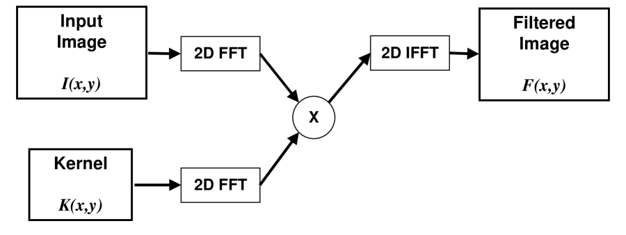
Figure 2: Basic 2D Filtering. FFT implementation of 2D filtering which performs the mathematical operation: $F(x,y)=\int\int K(x^{\prime},y^{\prime})I(x-x^{\prime},y-y^{\prime})dx^{\prime}dy^{\prime}$

where ${\vec{x}}=(x,y)$ and ${\vec{k}}=(k_{x},k_{y})$. Thus, in the discrete case we can compute the convolution using the standard discrete 2D $FFT$ and 2D $FFT^{-1}$ functions (see Figure 2)

$$F=FFT^{-1}(FFT(K)FFT(I))$$ (5)

which has a computation cost of $O(\log_{2}(M+N)^{2}$) operations per pixel, which, as will be shown later, can be reduced to $O(\log_{2}N^{2})$. [Traditionally, it has been necessary to pad the image out to the nearest power of 2 in order to exploit optimized implementations of the FFT. This limitation can easily result in “excessive” padding in many image processing applications. For example, a 560 x 300 image may need to be padded out to 1024 x 512, which is an increase of over 300%. However, more recently, self-optimizating implementations of the FFT (e.g. FFTW [2, 8] allow high performance for non-powers of two to be obtained without additional software tuning by programmers (see Appendix A).]

2.2 Convolution with Variable Kernels

As mentioned earlier, one of the primary drivers towards a more software centered image processing pipelines is increased complexity. One example of this type of complexity occurs in wide field of view imaging where filtering of large images via 2D convolutions is often complicated by a non-uniform point response function or kernel. For example, suppose the kernel function is itself sampled over an $N_{K}$ x $N_{K}$ grid on the image, so that $K_{ij}(x,y)$ represents the kernel centered on the $i,j$ point in the grid (Note: these indices are not the same as the pixel indices used in the previous section). The algorithm for dealing with this case is well known and the particular approach used here is based on the “overlap-and-add” method [12] for FFT based filtering. For discussion purposes the algorithm is first presented for “1D” images and then the 2D algorithm is describe (the method can be generalized to arbitrary dimensions, but that is not done here).

2.2.1 1D Case

Consider a 1D image to be filtered by a kernel which is sampled at two points $K_{1}(x)$ and $K_{2}(x)$. The true kernel at any point can be approximated by the weighted average of the two

$$K(x^{\prime})=W_{1}(x)K_{1}(x^{\prime})+W_{2}(x)K_{2}(x^{\prime})$$ (6)

where $W_{1}(x)=(x-x_{1})/(x_{2}-x_{1})$ and $W_{2}(x)=1-W_{1}(x)$. Thus, filtering with this kernel becomes

$$F(x) = \int K(x^{\prime})I(x-x^{\prime})dx^{\prime}~{},$$ (7)

$$= \int[W_{1}(x)K_{1}(x^{\prime})+W_{2}(x)K_{2}(x^{\prime})]I(x-x^{\prime})dx^{\prime}~{},$$

$$= W_{1}(x)\int K_{1}(x^{\prime})dx^{\prime}~{}~{}+~{}~{}W_{2}(x)\int K_{2}(x^{\prime})I(x-x^{\prime})dx^{\prime}~{}.$$

In other words, convolving with a variable kernel is equivalent to convolving with each kernel individually and combining the results with appropriate weightings.

2.2.2 2D Case

2D images are a straightforward extension of the above case

$$F(x,y)=\sum_{i=0}^{N_{K}-1}\sum_{j=0}^{N_{K}-1}W_{ij}(x,y)\int\int K_{ij}(x,y)I(x-x^{\prime},y-y^{\prime})dx^{\prime}dy^{\prime}~{}.$$ (8)

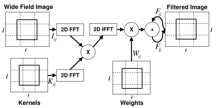
Figure 3: Wide Field Filtering. FFT implementation of 2D filtering for wide field imaging with multiple point response functions. Each portion of image is filtered separately and then recombined using the appropriate weights. The equivalent mathematical operation is: $F_{ij}(x,y)=W_{ij}(x,y)\int\int K_{ij}(x^{\prime},y^{\prime})I_{ij}(x-x^{\prime},y-y^{\prime})dx^{\prime}dy^{\prime}$

Or, more explicitly, if $I_{ij}$ and $F_{ij}$ are the regions of $I$ and $F$ that are affected by $K_{ij}$, then we can compute each $F_{ij}$ separately using FFT-based methods and then add it to the overall image using the appropriate weightings (see Figure 3).

The above derivation is intended to be a rough outline of the classic FFT based approach to 2D convolutions. Many details have been left out (e.g., real vs. complex FFTs, zero padding, treatment of edge effects, etc …). For a more precise description of the details necessary to implement the above algorithm see Appendix B.

3 Parallel Scheme

The previous section presented a general algorithm for efficiently convolving 2D images. Up to this point, there has been no mention as to how to implement this algorithm on a parallel computer. There are many potential “degrees of parallelism” available at the coarse, medium and fine grain level. These levels of parallelism can be described as follows

Image

The highest level of parallelism potentially exists at the application level. It may be the case that multiple independent images are to be filtered in a sequence. Exploiting this task level parallelism (sometimes referred to as “round robining”) is very efficient, but is application specific and leads to long turnaround times for each image (i.e. high latency).

Sub-image

Convolving with multiple kernels (or breaking up a single convolution into multiple smaller convolutions) leads to a natural breakup of the larger image into sub-images. This type of decomposition is sufficiently commonplace that it is reasonable to exploit this level of parallelism. This level of parallelism is relatively coarse grain because the $I_{ij}$, $K_{ij}$, $W_{ij}$, and $F_{ij}$ can all be computed independently. In addition, this level of parallelism can be abstracted away from the user.

Row/Column

Within each image, it is possible to perform the convolutions first by row and then by column (or vice versa). This offers a very large number of degrees of parallelism. However, this method is complicated by the need to transpose or “corner turn” the data between steps, which can introduce large communication costs. Furthermore, this method requires working beneath the 2D FFT routine, thus significantly increasing the coding overhead.

Instruction

The lowest level of parallelism that can be exploited is at the instruction level. This normally requires hardware support and is beyond the scope of this work.

The selection of which level(s) of parallelism to employ is based on a detailed analysis of the computation, communication, load balancing and software overheads incurred. These overheads are summarized in Table 1. Based on this analysis, exploiting the natural decomposition of the larger image into sub-images was selected. In this scheme each sub-image $I_{ij}$ is sent to a different processor (see Figure 3. The approach has a variety of advantages, not the least of which is that it can be implemented within the scope of a math library and does not impose upon the application (see next section). The rest of this section will present a more detailed analysis of the overheads of this approach.

3.1 Computation Cost

The computational cost of implementing an FFT based convolution is dominated by the two forward and one inverse 2D FFTs (i.e. three FFTs total). In addition, each sub-image of the filtered image will be a weighted sum of the convolution of the four neighboring kernels. The cost per sub-image is $4\cdot 3\cdot 5N^{\prime 2}\log_{2}N^{\prime 2}$, where $N^{\prime}=N+M/N_{K}$ is the size each padded sub-image (Note: this padding is due to edge effects and is unavoidable). This cost can usually be reduced by performing the FFT of the kernel in advance, and by exploiting the fact that the images are real valued and not complex. Using these techniques, the computational cost can be reduced to $4\cdot 5N^{\prime 2}\log_{2}N^{\prime 2}$. The cost for computing the entire image is $N_{K}^{2}$ times this value or $4\cdot 5N_{K}^{2}N^{\prime 2}\log_{2}N^{\prime 2}$.

One advantage of the sub-image parallel approach is that it is independent of the underlying method of performing the convolutions. A direct summation approach can be used and may be more efficient in the case of very small kernels. If a direct summation approach is used, this would require $4\cdot 2N_{K}^{2}N^{\prime 2}N^{2}$ operations. The “turnover” point between direct summation and FFT based methods occurs when $2N^{2}=5\log_{2}N^{\prime 2}$. In the case where $N_{K}$ is large and $M/N_{K}\approx N$, and $N^{\prime}\approx 2N$, then the turnover point occurs when

$$4\cdot 5N_{K}^{2}N^{\prime 2}\log_{2}N^{\prime 2}=4\cdot 2N_{K}^{2}N^{\prime 2}N^{2}$$ (9)

or

$$N^{2}=5\log_{2}(4N).$$ (10)

In other words, if $N>8$ then it is more efficient to use an FFT based approach. [This estimate is only a guideline as many other system specific factors (cache architecture, vector size, pipeline depth, etc …) effect the precise performance of these operations.]

3.2 Communication Cost

The impact of communication depends upon the distributions of the input and output images and the memory and networking architecture of the parallel computer.

In the expected case, communication costs of this approach are dominated by the initial sending of data to each processor and the final assembly of the filtered sub-images into one image. Because of edge effects, slightly more than the entire image needs to be sent to the individual processors, $N^{\prime 2}$ pixels per sub-image or $N_{K}^{2}N^{\prime 2}=M^{2}+N_{K}^{2}N^{2}$ pixels in total. To assemble the final image, there are no edge effects, but requires summing up to four separate sub-images or $4M^{2}$ pixels total.

In the best case, if each sub-image is initially distributed onto a processor the initial sending of data reduces to sending the overlapping edge data or $N_{K}^{2}N^{2}$ pixels, and the final assembling of data will be reduced to $3M^{2}$ pixels (not a large change from the expected case).

In the worst case, all of the data reside on a single processor, which doesn’t change the amount of data transmitted (as compared to the expected case), but can lead to a bottleneck due to the finite link bandwidth into and out of a single processor.

These communication costs, when combined with computation costs leads to a computation to communication ratio of

$$R=\frac{{\rm Computation}}{{\rm Communication}}=\frac{20N_{K}^{2}N^{\prime 2}\log_{2}N^{\prime 2}}{N_{K}^{2}N^{\prime 2}+4M^{2}}.$$ (11)

In the case where $N_{K}$ is large and $M/N_{K}\approx N$, and $N^{\prime}\approx 2N$ then $M\approx\frac{1}{2}N_{K}N^{\prime}$, and

$$R\approx\frac{20N_{K}^{2}N^{\prime 2}\log_{2}N^{\prime 2}}{N_{K}^{2}N^{\prime 2}+N_{K}^{2}N^{\prime 2}}=10\log_{2}N^{\prime 2}~{},$$ (12)

which for a typical value (e.g., $N^{\prime}=256$) leads to a computation to communication ratio of 160, which indicates that reasonably good parallel speedups should be possible with this parallel scheme.

More specifically, the parallel speedup can be roughly modeled as

$${\rm Speedup}=\frac{T_{\rm Comp}}{T_{\rm Comp}/N_{P}+T_{\rm Comm}}=\frac{(T_{\rm Comp}/T_{\rm Comm})}{(T_{\rm Comp}/T_{\rm Comm})/N_{P}+1}=\frac{\alpha^{-1}R}{\alpha^{-1}R/N_{P}+1}$$ (13)

where $N_{P}$ is the number processors, $T_{\rm Comp}/T_{\rm Comm}=\alpha^{-1}R$, and $\alpha$ parameterizes the performance of the parallel computer

$$\alpha=\frac{\rm Efffective~{}Processor~{}Speed}{\rm Effective~{}Link~{}Bandwidth}\approx\frac{0.15({\rm Peak~{}Speed})}{0.5({\rm Peak~{}Bandwidth})}~{}.$$ (14)

For a typical loosely connected parallel computer such as a cluster $\alpha\approx 3$ flop/byte. In such a system, the maximum speedup obtainable ($N_{P}\rightarrow\infty$) is $\alpha^{-1}R\approx 50$. For a more tightly coupled system $\alpha\approx 1$ and the maximum speedup is closer to 150.

3.3 Load Balancing

Load balancing is critical to the effective use of a parallel system. Finite images with edges introduce load imbalances. The four corner sub-images will have to do only one quarter of the processing and the $4(N_{K}-2)$ edge sub-images will have roughly one half the processing of the $(N_{K}-2)^{2}$ interior sub-images. In addition, if the image is not square additional imbalances will occur. Depending on the distribution of the data, the amount of time it will take to communicate to different processors depends on their location within the computer, which can lead to further imbalances.

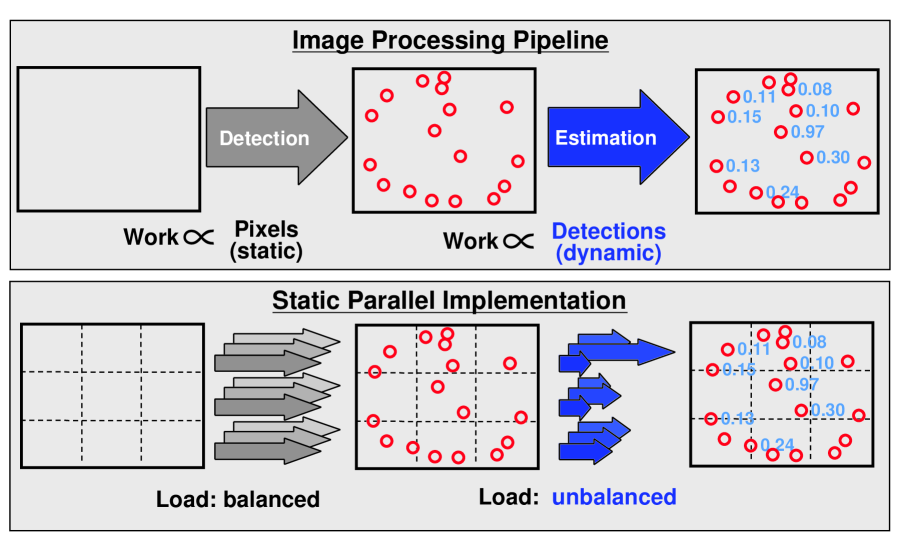
Figure 4: Load Imbalance. Pre-detection the work in a pipeline is usually a simple function of the number of pixels. Post-detection the work is usually a simple function of the number of detections. In a statically parallel system, statistical fluctuations in the number of detections will lead to a load imbalance in the post detection processing.

In addressing these load balancing issues, it is worthwhile to consider how filtering is used within the overall image processing chain (see Figure 4). It is often the case that filtering immediately precedes the detection stage in an image processing pipeline, which marks the boundary between the deterministic and stochastic processing loads. Before detection, the amount of processing is simply a function of the size of the input image and can be determined in advance. After detection, the work load is proportional to the number of detections which are randomly distributed.

Randomly distributed loads are a challenging and well studied problem [11]. In general, dynamic load balancing is required in order to effectively handle these types of problems (see Appendix C). Dynamical load balancing approaches often use a central authority to assign work to processors as they become available. Thus, from a higher level system perspective, given the need for dynamic load balancing approaches in the system, it is worthwhile to exploit them to handle the deterministic load imbalance introduced by edge effects.

The parallel algorithm employed here lends itself to dynamic load balancing for two reasons. First, the input data is never modified and can be broadcast in any order. Second, the final assembly consists of weighted sums which can also be performed in any order. The ability perform operations out of order allows a great deal of flexibility in pursuing dynamic load balancing techniques. Of course, the price for employing these mechanisms is the need for the underlying hardware and software technologies that support them, such as shared memory and multi-threading.

3.4 Software Costs

As mentioned earlier, one of the primary benefits of parallelizing over the sub-images is that it allows all the parallel complexity be implemented in a way that is hidden from the user. Thus this parallel convolution function can be implemented with a very simple signature

       filtered_image = convolve(input_image,kernels,n_processors)

Such a lightweight application level signature places all of the burden of the implementation into the library, but this burden can be significantly eased by employing existing open standards for doing high performance mathematical operations and thread based parallelism (see next section)

4 Software Architecture

The previous sections presented and analyzed an algorithm and parallel scheme for image filtering operations. The analysis indicates that significant speedups should be possible with this approach. However, this potential will be of limited value unless it can be incorporated into an effective software architecture, which addresses the issues of portability, performance and productivity. This section describes how these issues are addressed for the 2D convolution algorithm, using software techniques that are generally applicable to a wide variety of algorithms.

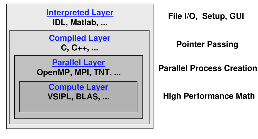
Figure 5: Layered Software Architecture. The user interacts with the top layer which provides high level abstractions for high productivity. Lower layers provide performance via parallel processing and high performance kernels.

The key to supporting a parallel algorithm with effective software is to use a layered approach with each layer addressing a different system requirement (see Figure 5). At the top level a high level interpreted language (such as IDL or Matlab) is used. This allows for rapid integration of the parallel 2D convolver into a high productivity environment by simply adding a function call to these environments. The next layer is the parallel library layer (in this case OpenMP) which provides access to thread-based parallelism using an open portable standard. The lowest level is the computation layer where the actual mathematical operations are performed. Here the Vector, Signal, and Image Processing Library (VSIPL) standard is used to provide high performance computations using an open standard. Both the OpenMP and VSIPL standards have enormous potential to allow users to realize the goal of portable applications that are both parallel and optimized.

VSIPL is an open standard C language Application Programmer Interface (API) that allows portable and optimized single processor programs. This standard encompasses many core mathematical functions including FFT and other signal processing operations which are essential for 2D filtering. In addition, VSIPL provides strong support for early binding and in place operations which allows the overhead of setup and memory allocation to be dealt with outside of the time critical part of the program.

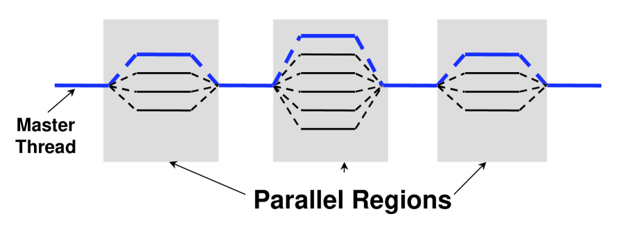
Figure 6: Multi-threaded Program. OpenMP uses a fork/join model in which a master thread forks off multiple parallel threads, which rejoin to communicate or synchronize (figure adapted from [7])

OpenMP [9] is an open standard C/Fortran API that allows portable thread based parallelism on shared memory computers. OpenMP uses a basic fork/join model (see Figure 6) wherein a master thread forks off threads which can be executed in parallel and rejoins them when communication or synchronization is required. This very simple model allows for a large program to be parallelize quickly with the insertion of a small number of compiler pragmas. As described earlier thread based parallelism is advantageous for two reasons. First, it is highly amenable to dynamic load balancing schemes. Second, it is easily implemented underneath higher level environments because it based on dynamic process creation and does not require a priori process creation or multiple invocations of the higher level library.

Exploiting these new open standards requires integrating them into existing applications as well as using them in new efforts. Image processing is one of the key areas where VSIPL and OpenMP can make a large impact. Currently, a large fraction of image processing applications are written in the Interpreted Data Language (IDL) environment [3]. A goal of this work is to show that it is possible to bring the performance benefits of these new standards to the image processing community in a high level manner that is transparent to the user. IDL, like most interpreted languages, does not have parallel constructs, but has a simple means for linking to externally built library functions. This mechanism allows the user to write functions in Fortran, C or C++ to obtain better performance. In addition, it is possible to link in other high performance and parallel libraries in a manner that is independent of the calling mechanism.

There are many opportunities for parallelism in this algorithm. The one chosen here is to convolve each kernel separately on a different processor and then combine all the results on a single processor. At the top level a user passes the inputs into an IDL routine which passes pointers to an external C function. Within the C function OpenMP forks off multiple threads. Each thread executes its convolution using VSIPL functions. The OpenMP threads are then rejoined and the results are added. Finally a pointer to the output image is returned to the IDL environment in the same manner as any other IDL routine.

5 Results

The inputs of image convolution with variable kernels consists of a source image, a set of kernel images, and a grid which locates the center of each kernel on the source image. The output image is the convolution of the input image with each PRF linearly weighted by its distance from its grid center. Today, typical images sizes are in the millions (2K x 2K) to billions (40K x 40K) of pixels. A single kernel is typically thousands of pixels (100 x 100) pixels, but can be as small 10 x 10 or as large as the entire image. Over a single image a kernel will be sampled as few as once but as many as hundreds of times depending on the optical system.

The parallel convolution algorithm presented here was implemented on an SGI Origin 2000 at Boston University. This machine consists of 64 300 MHz MIPS 10000 processors with an aggregate memory of 16 GBytes. IDL version 5.3 from Research Systems, Inc. was used along with SGI’s native OpenMP compiler (version 7.3.1) and the TASP VSIPL implementation. Implementing the components of the system was the same as if each were done separately. Integrating the pieces (IDL/OpenMP/VSIPL) was done quickly, although care must be taken to use the latest versions of the compilers and libraries. Once implemented the software can be quickly ported via Makefile modifications to any system that has IDL, OpenMP, and VSIPL (currently these are SGI, HP, Sun, IBM, and Red Hat Linux).

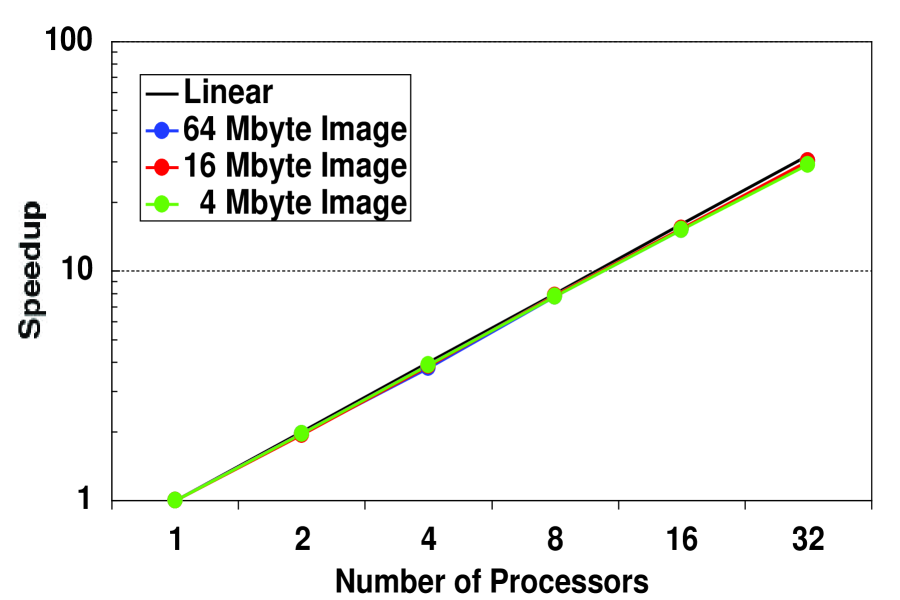
Figure 7: Parallel Speedup. Measured speedups of wide field 2D filtering application on an shared memory parallel system (SGI Origin2000).

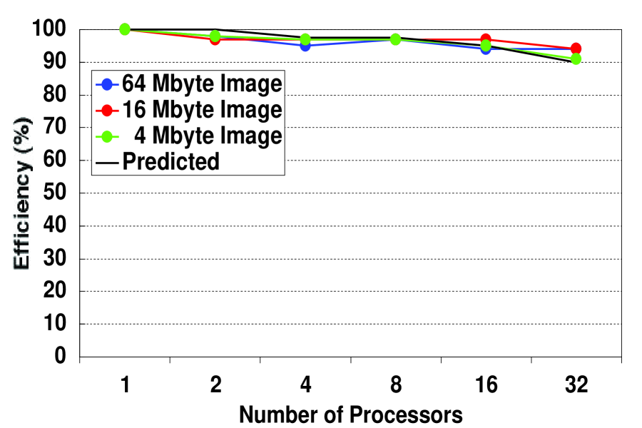
Figure 8: Parallel Efficiency. Measured parallel efficiency of wide field 2D filtering application on an shared memory parallel system (SGI Origin2000).

The performance of this implementation was tested by timing the program over a variety of inputs and numbers of processors. The measured speedups were computed by dividing the parallel times by the single processor times (see Table 2 and Figure 7). In all cases, the kernel size was $N=100$ and the padded sub-image size was $N^{\prime}=512$. The resulting computation to communication ratio obtained from Equation 11 was $R=288$. Assuming $\alpha\approx 1.0$ and inserting this value of $R$ in Equation 13 gives predicted speedups of 2.0, 3.9, 7.8, 15.2, and 28.8 on 1, 2, 4, 8, 16 and 32 processors, respectively The measured and predicted parallel efficiencies (speedup/number of processors) are shown in Figure 8, and are good agreement.

6 Conclusions

Image filtering via 2D convolutions is often the dominant image processing operation in terms of computational cost. This work has looked at three ways of improving performance of 2D convolutions in a software centered image processing environment: better algorithms, better optimization and parallel processing. The result is a general FFT based algorithm for implementing 2D convolutions, which is also well suited for wide field of view images. The algorithm uses a parallel scheme which minimizes the communication overhead and allows for dynamic load balancing. The algorithm has been implemented using a general purpose software architecture for transparently integrating it within high level image processing environments. This implementation exploits the OpenMP and VSIPL standards. We have conducted a variety of experiments which show linear speedups using different numbers of processors and different image sizes (see Figures 7 and 8). Thus, it is reasonable to conclude that it is possible to achieve good parallel performance using open standards underneath existing high level languages.

This general approach is not limited to IDL but can be extended to most interpreted languages (e.g., Matlab, Mathematica, …). Extending this approach to other environments and implementing a variety of important signal processing kernels (e.g. pulse compression, adaptive beam-forming, …) has enormous potential for enabling easy to use high performance parallel computing.

The author is grateful to Glenn Breshnehan, Kadin Tsang and Mike Dugan of the Boston University Supercomputer Center for their assistance in implementing the software; to Randy Judd and James Lebak for their assistance with the VSIP Library; to Charlie Rader for helpful comments on 2D FFTs; to Matteo Frigo and Steve Johnson for their assistance with FFTW; to Paul Monticciolo for his help with the text and to Bob Bond for his overall guidance.

A Optimal padding of FFTs

Parallel implementations of any algorithm need reliable models for the underlying computations. The standard computational cost of a complex FFT of length $N$ is $5N\log_{2}(N)$. The FFT can be implemented with a variety radixes, but normally base 2 is the simplest to optimize. In a typical optimized FFT implementation powers of two FFT sizes usually offer a significant performance boost over other sizes. Furthermore, because of the butterfly data access patterns of the FFT, the performance penalty of using a non-optimized FFT can be quite large (especially on a computer with a multi-level cache). Given this situation, it has been standard practice to “pad” the FFTs out to the nearest power of two $N^{\prime}=2^{\lceil\log_{2}(N)\rceil}$.

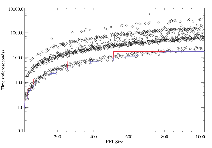
Figure 9: FFTW performance. Performance of FFTW on FFTs ranging in size from 16 to 1024. The blue line indicates the performance achieved using the optimally padded FFT. The red line shows the performance obtained using powers of two.

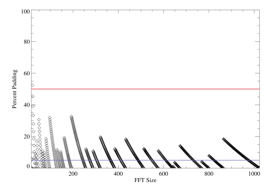
Figure 10: FFTW Optimal Paddings. Optimal padding (as a percentage of FFT size). The ability to get good performance with non-powers of two significantly reduces the amount of padding required. The blue line indicates the average padding require across all the different cases. The red line shows the average padding required if only powers of two are used.

Fortunately, the advent of self-optimizing software libraries such as FFTW now significantly reduce the software engineering cost of optimizing non-standard length FFTs. Figure 9 shows the times for different length FFTs using FFTW, and the results of using the optimal amount of padding. The amount of padding and the performance gains of using this padding are shown in Figure 10. The performance gained using a non-powers of two FFT are shown in Figure 11. These results indicate that while some padding is still a good idea, it is usually quite modest ($\sim$5%). Given this situation it is now quite reasonable to estimate FFT performance using unpadded values.

B 2D Convolution Algorithm Description

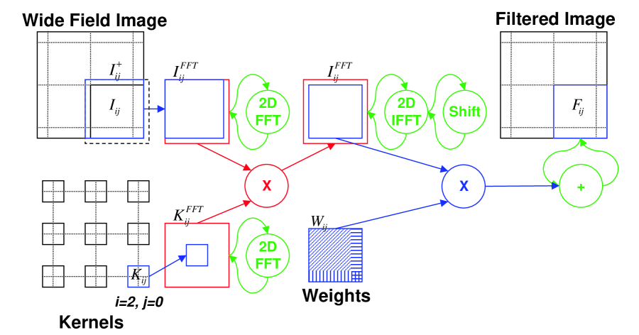
Figure 12: Detailed Algorithm Flow. Precise computations, data structures and data movements necessary to execute 2D convolution algorithm with multiple kernels. The inputs consist of the image to be filtered and a grid with a kernel at each node. The algorithm proceeds by looping (in parallel) over each kernel in the grid $K_{ij}$ and executing the following steps:

Section 2 provided a high level description of using FFTs for 2D convolution with variable kernels. This appendix is meant to provide the more specific details necessary for implementation. Figure 12 presents pictorially the precise computations, data structures and data movements necessary to execute 2D convolution algorithm with multiple kernels. The inputs consist of the image to be filtered and a grid with a kernel at each node. The algorithm proceeds by looping (in parallel) over each kernel in the grid $K_{ij}$ and executing the following steps:

• Determine boundaries of input sub-image $I_{ij}$. Using kernel grid determine area affected by kernel $K_{ij}$.

• Compute corresponding weights $W_{ij}$. Determine number of kernels contributing to each part of the sub-image. Linearly weight each pixel by its distance from the center of kernel.

• Determine boundaries of filtered sub-image $F_{ij}$ (same as relative position as $I_{ij}$).

• Determine boundaries of sub-image padded by kernel $I^{+}_{ij}$ by adding N/2 pixel border to $I_{ij}$.

• Determine size of and create padded sub-image $I^{FFT}_{ij}$ by padding $I^{+}_{ij}$ out to an optimal FFT size (see Appendix A).

• Create padded kernel $K^{FFT}_{ij}$ (same size as $I^{FFT}_{ij}$).

• Copy $I^{+}_{ij}$ into $I^{FFT}_{ij}$ so that sub-image $I_{ij}$ is in the center.

• Copy $K_{ij}$ to center of $K^{FFT}_{ij}$.

• In place 2D FFT $I^{FFT}_{ij}$.

• In place 2D FFT $K^{FFT}_{ij}$.

• Multiply $I^{FFT}_{ij}$ by $K^{FFT}_{ij}$ and return to $I^{FFT}_{ij}$.

• In place 2D IFFT $K^{FFT}_{ij}$.

• In place 2D circular Shift $I^{FFT}_{ij}$. Full half shift in both x and y directions.

• Multiply $I^{FFT}_{ij}$ sub-region corresponding to $I_{ij}$ by $W_{ij}$ and add to $F_{ij}$.

C Dynamic Load Balancing “Balls into Bins”

The classic “Balls into Bins” problem has been well studied (see [10, 1] and references therein). In this appendix results are derived for this classic problem as it pertains to pipeline image processing. The notation used in this section is different from the main body of the text, but consistent with what is used in the wider literature where $M$ is the number of “balls” (i.e., the amount work to be done) and $N$ is the number of “bins” (i.e., the number of processors that can be used).

In an image processing context $M$ is the average number of detections that can be expected in a given image. In a parallel processing pipeline, the image will be divided up into $N$ sub-images. Let $\lambda=M/N$ be the expected number of detections in each sub-image, and $p_{\lambda}(m)$ be the probability that that a given sub-image will have exactly $m$ detections. Likewise, let $P_{\lambda}(m)=\sum_{m^{\prime}=0}^{m}p_{\lambda}(m^{\prime})$ be the probability that a given sub-image has up to $m$ detections in it.

In most analysis of this type the focus is on the expected maximum number of “balls” that would fall in a given “bin.” In a real-time image processing pipeline environment, it is more typical to work with the function $M_{f}$ which is the number detections at a given a failure rate $f$. In other words, $f$ is the probability that a given processor in the system will have more than $M_{f}$ detections to process. This approach is necessary in order to bound the amount of work that is allowed to during the detections step so as not to miss any real-time deadlines. In general, $M_{f}$ is given by the following equation

$$P_{\lambda}(M_{f})^{N}=1-f$$ (15)

Finding $f$ for a given value of $M_{f}$ is simply a matter of evaluating $P_{\lambda}$. Finding $M_{f}$ for a given $f$ is slightly more difficult but can be accomplished by using the following coupled recursive equations

$$N_{f}^{0} = 0$$

$$P^{0} = p_{\lambda}(N_{f}^{0})$$

$$N_{f}^{i+1} = \{N_{f}^{i}+1:P^{i}<(1-f)^{N}$$

$$P^{i+1} = \{P^{i}+p_{\lambda}(N_{f}^{i+1}):N_{f}^{i+1}>N_{f}^{i}$$ (16)

The above formula will work for arbitrary $p_{\lambda}$, but typically we are interested in the case where the detections are independent random events and $p_{\lambda}$ follows a Poisson distribution

$$p_{\lambda}(m)=\frac{\lambda^{m}e^{-\lambda}}{m!}$$ (17)

In this case, $P_{\lambda}$ is given by the unnormalized incomplete Gamma function

$$P_{\lambda}(m)=\tilde{\Gamma}(m+1,\lambda)=\frac{\Gamma(m+1,\lambda)}{m!}~{},$$ (18)

where $\Gamma$ is the incomplete Gamma function given by the following sum

$$\Gamma(m+1,\lambda)=m!\sum_{m^{\prime}=0}^{m}\frac{\lambda^{m^{\prime}}e^{-\lambda}}{m^{\prime}!}~{}.$$ (19)

Thus, $M_{f}$ can be computed by inverting the above function

$$M_{f}+1=\tilde{\Gamma}^{-1}((1-f)^{1/N},\lambda)$$ (20)

For a given $M_{f}$ the speedup on a parallel computer is given by

$${\rm Speedup}=\frac{M}{M_{f}}$$ (21)

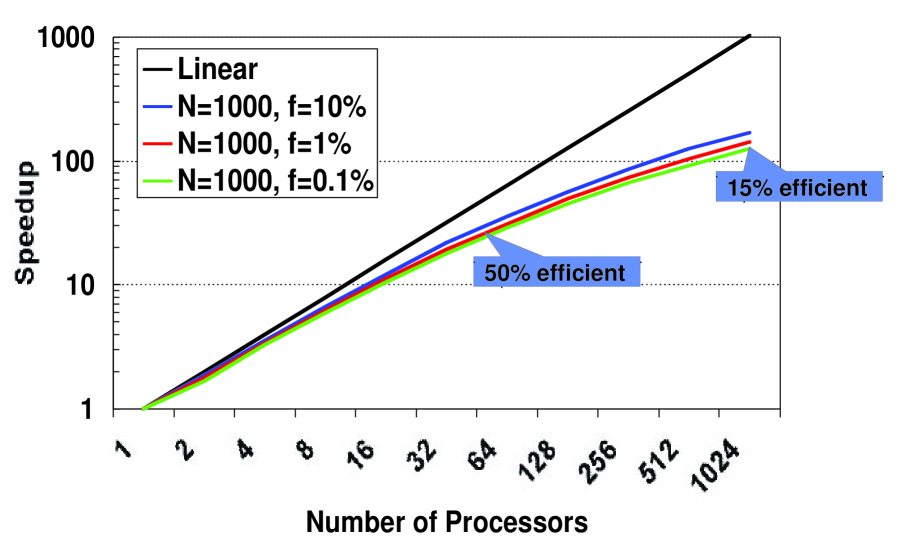
Figure 13: Static Speedup. Speedup obtainable for M=1000 tasks (“balls”) and given failure rates using a static assignment scheme. Random fluctuations significantly bound speedup.

If $M_{f}=\lambda$ then the speedup is linear. Random fluctuations in the distribution of detections will mean that some processors will have more detections resulting in sub-linear speedups. Figure 13 shows the speedup on various numbers of processors for different failure rates and indicates that even for a modest number of processors over half the processors will be idled due to load imbalances.

Alleviating the effects of random work loads requires adopting dynamic schemes that allow work to be assigned to processors as they become available. Assuming the work can be broken up with a granularity $g$ (i.e. the smallest amount of work is $gM$), then the worst case speedup ($f=0$) is given by

$${\rm Speedup}=\frac{M}{\lambda+gM}=\frac{M}{M/N+gM}=\frac{N}{1+gN}~{}.$$ (22)

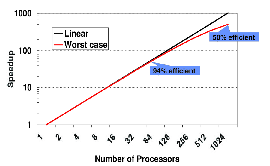
Figure 14: Dynamic Speedup. Speedup obtainable for M=1000 tasks and f = 0 using a dynamic work assignment scheme. This scheme provides good speedups even in the worst case.

Asymptotically, for large $N$ the speedup converges to $1/g$. Figure 14 shows the speedup obtainable using this type of strategy, which is significantly better than what can be obtained in the static situation.

Parallel	Compute Latency	Communication	Load	Software
Approach	Overhead	Overhead	Balancing	Overhead
Image	high	high	excellent	application
Kernel	medium	low	good	math library
Row/Column	low	high	good	math kernel
Instruction	low	unknown	excellent	OS/hardware

Table 1: Parallel Overheads. Computation, communication, load balancing and coding overheads for exploiting different levels of parallelism for doing a 2D convolution.

Image size	Kernel grid	Number of	Measured	Parallel
$M$	$N_{K}$	Processors	Speedup	Efficiency (%)
1024	8	1	1.00	100
1024	8	2	1.96	98
1024	8	4	3.88	97
1024	8	8	7.76	97
1024	8	16	15.2	95
1024	8	32	29.0	91
2048	16	1	1.00	100
2048	16	2	1.93	97
2048	16	4	3.86	97
2048	16	8	7.79	97
2048	16	16	15.3	97
2048	16	32	30.1	94
4096	32	1	1.00	100
4096	32	2	1.95	98
4096	32	4	3.80	95
4096	32	8	7.73	97
4096	32	16	15.1	94
4096	32	32	30.1	94

Table 2: Parallel speedups. Measured parallel speedup and parallel efficiency obtained for different image sizes and different numbers of processors. In each case the kernel size was $N=100$.

Figure 11: FFTW Performance Benefit. The percentage performance improvement obtained using optimal padding compared to only powers of two.

• Determine boundaries of input sub-image $I_{ij}$.

• Compute corresponding weights $W_{ij}$.

• Determine boundaries of filtered sub-image $F_{ij}$.

• Determine boundaries of sub-image padded by kernel $I^{+}_{ij}$.

• Determine size of and create padded sub-image $I^{FFT}_{ij}$.

• Create padded kernel $K^{FFT}_{ij}$.

• Copy $I^{+}_{ij}$ into $I^{FFT}_{ij}$.

• Copy $K_{ij}$ to center of $K^{FFT}_{ij}$.

• In place 2D FFT $I^{FFT}_{ij}$.

• In place 2D FFT $K^{FFT}_{ij}$.

• Multiply $I^{FFT}_{ij}$ by $K^{FFT}_{ij}$ and return to $I^{FFT}_{ij}$.

• In place 2D IFFT $K^{FFT}_{ij}$.

• In place 2D circular Shift $I^{FFT}_{ij}$.

• Multiply $I^{FFT}_{ij}$ sub-region corresponding to $I_{ij}$ by $W_{ij}$ and add to $F_{ij}$.

These steps are described in greater detail in Appendix B.

References

- [1] P. Berenbrink, A. Czumaj, A. Steger and B. Vocking, Balanced Allocations: The Heavily Loaded Case, in “Proceedings of the 32nd Annual ACM Symposium on Theory of Computing,” pp 745-754, Portland, OR, May 21-23 2000. ACM Press, New York, NY.
- [2] M. Frigo and S. Johnson, FFTW: An Adaptive Software Architecture for the FFT, ICASSP Proceedings (1998), vol 3., p 1381.
- [3] Interactive Data Language by Research Systems, Inc. Boulder, CO http://www.rsi.com/
- [4] J. Kepner, M. Gokhale, R. Minnich, A. Marks and J. DeGood, Interfacing Interpreted and Compiled Languages to Support Applications on a Massively Parallel Network of Workstations (MP-NOW), Cluster Computing 2000, volume 3, number 1, page 66
- [5] J. Kepner Integration of VSIPL and OpenMP into a Parallel Image Processing Environment, J. Kepner, proceedings of the the fourth High Performance Embedded Computing Workshop (HPEC 2000), September 20-22, 2000, MIT Lincoln Laboratory, Lexington, MA
- [6] J. Kepner, Exploiting VSIPL and OpenMP for Parallel Image Processing, in “Proceedings of ADASS X” (editors), Boston, MA 2000
- [7] T. Mattson and R. Eigenmann, Parallel Programming with OpenMP, Supercomputing’99, Nov 13, 1999, Orlando, FL
- [8] C. Moler and S. Eddins, Faster Finite Fourier Transforms, Matlab News & Notes, Winter 2001
- [9] OpenMP: Simple, Portable, Scalable Programming, http://www.openmp.org/
- [10] M. Raab & A. Steger, Bins into Balls — A Simple and Tight Analysis In 2nd International Workshop on Randomization and Approximation Techniques in Computer Science (RANDOM’98), pages 159–170, 1998.
- [11] B. A. Shirazi, A R. Hurson, K. M. Kavi, Scheduling and Load Balancing in Parallel and Distributed Systems, IEEE Computer Society Press, 1995
- [12] T. G. Stockham, High Speed Convolution and Correlation, Spring Joint Computer Conference, AFIPS Proceedings, 28, pp 229-233, 1966
- [13] Vector, Signal, and Image Processing Library http://www.vsipl.org/