A revision of the solar neighbourhood metallicity distribution

Abstract

We present a revised metallicity distribution of dwarfs in the solar neighbourhood. This distribution is centred on solar metallicity. We show that previous metallicity distributions, selected on the basis of spectral type, are biased against stars with solar metallicity or higher. A selection of G-dwarf stars is inherently biased against metal rich stars and is not representative of the solar neighbourhood metallicity distribution. Using a sample selected on colour, we obtain a distribution where approximately half the stars in the solar neighbourhood has a metallicity higher than [Fe/H]=0. The percentage of mid-metal-poor stars ([Fe/H]$<$-0.5) is approximately 4 per cent, in agreement with present estimates of the thick disc.
In order to have a metallicity distribution comparable to chemical evolution model predictions, we convert the star fraction to mass fraction, and show that another bias against metal-rich stars affects dwarf metallicity distributions, due to the colour (or spectral type) limits of the samples. Reconsidering the corrections due to the increasing thickness of the stellar disc with age, we show that the Simple Closed-Box model with no instantaneous recycling approximation gives a reasonable fit to the observed distribution. Comparisons with the age-metallicity relation and abundance ratios suggest that the Simple Closed-Box model may be a viable model of the chemical evolution of the Galaxy at solar radius.

1 Introduction

The aim of this paper is to present and discuss a new metallicity distribution of the stellar material found in the solar neighbourhood. In recent years, several such metallicity distributions, constructed from various samples of solar neighbourhood dwarfs have been published [Rocha-Pinto & Maciel, 1996, Wyse & Gilmore, 1995, Flynn & Morell, 1997, Favata et al., 1997]. These studies have repeatedly pointed to a deficit of metal-poor stars relative to the simplistic but insightful Simple Closed-Box model (hereafter SCB model). However, since the early seventies, models have successfully fit the observed metallicity distribution by alleviating one or another assumption of the SCB model . Such fits are now routinely obtained with present day models of chemical evolution of the Milky Way [Chiappini et al., 1997, Prantzos & Silk, 1998] using a pletora of solutions, the most widely accepted being the infall model.
In view of the apparent easiness of these models to fit this constraint of chemical evolution, one may wonder why the deficit of metal-poor stars is regularly addressed, and why we intend to do so. One reason is that the completion of Strömgren surveys by Olsen (see Olsen (1983) and thereafter) has considerably extended the available data. Moreover, the coincidental publication of the $Hipparcos$ Catalogue now allows a clean definition of a complete sample of solar neighbourhood dwarfs.

A second reason is that the role of the thick disc is still unclear and difficult to evaluate : is the thick disc the first epoch of the disc formation ? Is it cogenetic to the Galaxy ? And how should it be taken into account when considering the G dwarf problem ? In the present study, we take the view that the thick disc is an integral part of the disc and that it should be considered when discussing the G-dwarf problem. This raises the question of the exact contribution of the thick disc at [Fe/H]$<$-0.4. Wyse & Gilmore (1995) have contended that the important metallicity tail below this limit ($>$20%) is likely due to contamination by the thin disc. This problem is then connected to another. If the thin disc contribution at [Fe/H]$<$-0.4 is as important as envisaged by Wyse & Gilmore (1995), it leads to the conclusion that the SFR must have been very efficient at early times in the disc. This conclusion is reinforced by the apparent rapid rise of metallicity in the age-metallicity relation [Scully et al., 1997] - leaving even less time to produce the material at [Fe/H]$<$-0.4. As a matter of fact, it is a feature common to most models with infall that they use a decreasing SFR, in accordance with the infall decay rate [Tosi, 1996]. In contrast, all recent determinations of the SFR history of the disc point to a constant, or even slightly increasing SFR [Haywood et al., 1997, Binney et al., 2000]. We show here that these apparent contradictions are mostly an effect of pre-Hipparcos data, and that the metallicity tail at [Fe/H]$<$-0.4 is drastically reduced with Hipparcos parallaxes.

Third, while chemical evolution models have increased considerably in complexity over the last decade, the sophisticated solutions envisaged to solve the ‘G-dwarf problem’ (such as infall, variable initial mass function, etc), are still essentially adhoc, and direct observational evidence favoring one or another alternative have remain extremely elusive. Infall models have focused most of the efforts of galactic chemical evolution studies in recent years, while relatively little attention has been devoted to other solutions. Since the G-dwarf problem remains the main (indirect) support for long time-scale gas accretion by the Milky Way disc, it is important to check the failure (or success) of no-infall models. Also, when considering scenarios where the thick disc is envisaged as a genuine galactic population (as is the case here), it must be born in mind that no-infall models may come as a more natural alternative. The existence of the thick disc, if considered as cogenetic, implies that a substantial stellar disc must have been in place at early times (Wyse, 2000 astro-ph/0012270). As remarked by Wyse, this suggestion could find some support or invalidation in a more general context, from studies of high redshift galactic discs [Brinchmann & Ellis, 2000].

Finally, another incentive for this work has been the (naive) realisation by the author that while models of chemical evolution predict distributions of stellar mass as a function of metallicity, previous studies of the dwarf metallicity distributions have only been able to give statistics of stars as a function of metallicity. The accurate positioning of the stars in the HR diagram allowed by $Hipparcos$ parallaxes permits the conversion from (colour, magnitude) to masses. It will be demonstrated that, while the conversion itself has a relatively minor effect, the colour limits of the sample bias the distribution by underestimating the contribution of solar-metallicity and metal-rich stars.

The remainder of the paper is divided into 5 parts. In the following section, we present the calibrations used to estimate metallicity from Geneva and Strömgren photometry. After selecting a basic sample from considerations of completeness and available photometry, we select long-lived stars and discuss the biases introduced by our selection procedure. A first estimate of a corrected metallicity distribution of star frequency distribution is given. This distribution is then compared to previous works in section 3, where we also discuss the problem of biases in other samples. We evaluate the proportion of X-ray emitter stars in the sample. Since X-ray coronal activity is usually considered as a tracer of young stars, we discuss the significance of the high percentage of young star candidates in the sample. In section 4 we convert our dwarf metallicity distribution to a mass metallicity distribution. A proper correction for the mass bias and a final metallicity distribution are given for both iron and oxygen abundances. In section 5, we briefly review the observed parameters of the disc that enter the SCB model, and following Occam’s Razor, we explore how the Simple model fits other local constraints of chemical evolution. We conclude in the last section.

2 The observed dwarf metallicity distribution

2.1 Description of the sample

The solar neighbourhood, as sampled by the Hipparcos Catalogue, is considered to be essentially complete to $M_{v}$=8.5 for stars with $\pi>$40 mas [Jahreiss & Wielen, 1997], and contains 959 entries within these limits. At $M_{v}$=8.5, main sequence stars have $B-V$ colour between 1.3 and 1.5. Present day available photometric metallicity calibrations are limited to bluer colour. The Geneva photometric system is probably the best suited system in that regard, since the calibration is available down to $B_{2}-V_{1}$=0.65 [Grenon, 1978], corresponding to $B-V$=1.05 approximately. According to the available data, the main sequence of the galactic globular cluster M92 ([Fe/H]$\approx$-2) passes through the point B-V=1.00, M_v=8.0 [Stetson & Harris, 1988]. This means that the limit at M_v=8.5 is unlikely to produce any significant bias against low metallicity stars in the sample.

Within these limits, the sample contains 681 entries. If we further select stars with M${}_{v}>$3.5 and $B-V>$0.25 and which are not flagued as either G, O, S, or V suspected binaries, we find 475 entries, of which 82 are flagued “C” component solutions in the main catalogue. For 27 of these 82 systems, no Geneva photometry is available from the General Catalogue of Photometric Data [Mermilliod et al., 1997]. Those “C” component solutions for which photometry is available are usually not separated or simply not detected as binaries in the GCPD data base (except for 3 systems, for which photometry for the primary is available). We decided therefore to exclude entries with the flag “C” from further consideration, keeping in mind that we are however excluding a minimum of 82 stars with $B-V<$1.05 from our sample. We are then left with 393 stars for which iron abundance estimates are necessary.

2.2 Photometric metallicity calibration

When dealing with the metallicity distribution of stars in the solar neighbourhood, one is interested by long-lived stars down the main sequence, in order to avoid bias favoring young – and possibly more metal-rich – objets. However, metallicity measurements and calibration of M stars are still in infancy, and one is limited to stars bluer than M spectral type. There is no one single metallicity indicator for all the stars in the samples analysed in Sec. 3 and 4 and we rely on Strömgren or Geneva photometric metallicity, and for a few stars on spectroscopic data. We discuss herebelow the photometric calibrations we use, by reference to spectroscopic measurements.

2.2.1 Geneva photometric calibration for dwarfs : Grenon (1978)

A metallicity calibration of Geneva colour indices exists for main sequence stars down to $B_{2}-V_{1}$=0.65 ($B-V$=1.05) [Grenon, 1978]. Towards hotter main sequence stars, this calibration is valid up to $B_{2}-V_{1}$=0.4. The metallicity is related to the index $\delta_{1256}$, defined as the difference between the $U-B$ Geneva colour index of the star and the Hyades sequence at the $B_{2}-V_{1}$ colour of the star (see Grenon (1978)). This calibration is :

[Fe/H]_Gen=2.96+2.04/($\delta_{1256}$-0.72).

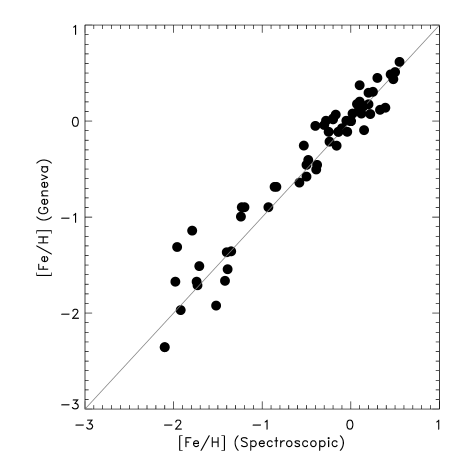
Figure 1: Photometric determination of metallicity using the calibration by [Grenon, 1978], versus spectroscopic measurements for dwarfs with 0.40$<$ B₂-V₁ $<$ 0.65.

Figure 2: Strömgren metallicities versus spectroscopic metallicities. Photometric metallicities are derived from the calibration by [Schuster & Nissen, 1989].

Numerous spectroscopic metallicities have been published for G and K dwarfs since 1978, so that we can check how this calibration behaves compared with recent spectroscopic metallicity measurements. We gathered a sample of spectroscopic metallicities from the literature, selecting stars that have Geneva photometry and 0.40$<$B₂-V${}_{1}<0.65$ from [Edvardsson et al., 1993, Feltzing & Gustafsson, 1998, Flynn & Morell, 1997, Axer et al., 1995, Castro et al., 1997]. We added a sample of Hyades stars, with individual spectroscopic [Fe/H], as listed in Perryman et al. (1997). The total sample amounts to 76 stars.

Fig. 1 shows the correlation between the photometric and spectroscopic iron abundance in this sample. Dispersion increases for low metallicity stars, however the photometric metallicity still nicely correlates with spectroscopic metallicities, with no apparent large deviations. A least square fit to the points of Fig. 1 yields a regression curve of [Fe/H]_Geneva=1.002*[Fe/H]_Spectro+0.054, indicating that the photometric iron abundance may overestimate the spectroscopic iron abundance by an amount of 0.05 dex.

2.2.2 Strömgren metallicity scale

Most previous studies of the G-dwarf problem are based on Strömgren photometry, it is therefore interesting to see how Strömgren metallicity calibration compares with respect to the Geneva photometric metallicity and to the spectroscopic scale. We apply the calibration given by Schuster & Nissen (1989) :

$$[Fe/H]=1.052-73.21m_{1}+280.9(b-y)m_{1}+$$

$$333.95(b-y)m_{1}^{2}-595.5(b-y)^{2}m_{1}+(5.486-$$

$$41.62m_{1}-7.963(b-y)(log(m_{1}-c_{3}))$$ (1)

when 0.22$<b-y<$0.375

$$[Fe/H]=-2.0965+22.45m_{1}-53.8m_{1}^{2}-62.04m_{1}b-y+$$

$$145.5m_{1}^{2}(b-y)+(85.1m_{1}-13.8c_{1}-137.2m_{1}^{2})*c_{1}$$ (2)

when 0.375$<b-y<$0.59.

The indix c3 is defined as $c3=0.6322-3.58(b-y)+5.20(b-y)^{2}$

Fig. 2 shows the spectroscopic vs Strömgren photometric determination of [Fe/H] for an enlarged sample of 110 stars, with the Strömgren metallicity calculated using the Schuster & Nissen (1989) calibration. A fit applied to this sample yields [Fe/H]_Stromgren=0.865[Fe/H]_Spectro-0.052, indicating a problem in the calibration, a result similar to Alonso et al. (1996). The correction to this calibration suggested by these authors is 0.85 [Fe/H]-0.04, which is concordant with our fit.

Figure 3: Stars with Strömgren photometric iron abundance estimates (hashed histogram) and Geneva photometric abundance estimates (thick line histogram).

Of the 393 stars of our sample, 324 have Geneva photometry, 69 stars have not. Out of these 324 stars, 177 have 0.4 $<~{}$B₂-V₁ $<$ 0.65, and their metallicity can be estimated with the calibration of [Grenon, 1978]. Among the 147 stars with B₂-V₁ out of this interval, 9 stars have B₂-V₁ $>$ 0.65, and are not considered any further. We are left with 138 stars plus 69 stars which have no Geneva photometry. Out of these 207 objects, 166 have a Strömgren photometry, and the corrected calibration above can be applied. There are 41 stars for which no Strömgren nor Geneva photometry is available, and 7 of these have a metallicity in the catalogue of Cayrel de Strobel et al. (1997). Two stars with a position above the main sequence that suggest binarity have been removed. Our final sample has 348 stars with estimated iron abundance.

Fig. 3 shows the photometric [Fe/H] distributions of the two subsamples (Geneva and Strömgren photometric metallicities), and illustrates that they cover approximately the same [Fe/H] range, with a tendency for the ’Geneva’ sample to be more metal-rich. The colour criteria for the selection of the stars in each sample explains this difference, the objects in the ’Geneva’ sample are redder, and it is expected to favor metal-rich stars.

2.3 Age and mass biases

One of the predicted quantities of chemical evolution models of the galactic disc is the fraction of stellar mass as a function of metallicity. Ideally, a distribution also function of the age would be desirable, but since measurements of the age of (most) long-lived stars is impractical, such a distribution is still out of reach. However, because we observe metallicity to be a rough function of age, an unbiased sample must not favor any particular age, and in particular should not include short lived stars, which are only representative of recent chemical evolution.

A second bias, that has been neglected in previous determinations of the metallicity distribution, is introduced in observed samples by the fact that, due to selection criteria (e.g, colour limits or spectral types), the metallicity is not sampled over the same width of mass interval. The selection of long-lived stars and the colour limit imply that metal-rich stars are selected on a smaller mass interval than metal-poor stars. This would be of no consequence if chemical evolution models take this effect into account, but this is never done in practice. We review these 2 biases in turn.

2.3.1 Correcting for age bias

The selection of long-lived dwarfs is necessary to avoid bias favoring young stars in the sample, or recent galactic evolution. We are looking for those stars in the sample which would still be below the turn-off after a duration equal to the disc age. If the (thick and thin) disc age is 12 Gyr, this imply that the stars we are interested in have a main sequence mass lower than the turn-off mass of the 12 Gyr isochrone at the star metallicity, which we note M${}_{TO}^{*}$. In principle, because the stars in the sample may have any age between 0 and 12 Gyr, they must be located to the right of the evolutionary track with mass M${}_{TO}^{*}$, and to the left of the 12 Gyr isochrone.

In practice, these requirements are impossible to apply because (1) we don’t know the age of the disc to a satisfactory accuracy, (2) although excellent, $Hipparcos$ parallaxes are not sufficiently accurate to locate meaningfully the observed star between the isochrone and evolutionary track (3) theory of stellar evolution and the various transformations necessary to compare the observed star with isochrones and evolutionary tracks are still too imprecise. As a consequence, we have applied a simpler procedure which consisted in selecting stars to the right or below the evolutionary track with mass M${}_{TO}^{*}$. The turn-off mass is obtained from a 12 Gyr isochrone, which is taken here as the age of the galactic (thin and thick) disc. Lebreton (2000) has demonstrated that standard stellar evolution calculation shows differences of about 100–200 K compared with the best available data for deficient and mildly deficient stars. According to Lebreton (2000), these differences can be eliminated if (1) non-ETL corrections are applied to the metallicity data and (2) microscopic diffusion of heavy elements is accounted for in stellar models, which results in effective temperature shift of about 100-200 K. Before selecting the stars, we artificially applied an equivalent shift in metallicity to the observed sample, and in temperature to the stellar models.

Figure 4: Description of the sample of long-lived dwarfs (a) Iron abundance distribution. The upper histogram (thick line) is the sample before the selection of long-lived dwarfs. The (thin line) histogram counts the stars left after having selected long-lived stars. (b) HR diagram of selected stars. (c) For a given star in the sample, the abscissa gives the $B-V$ of the solar isochrone at the magnitude of the star, minus the $B-V$ colour of the star.

The selection of long-lived dwarfs, applied to the 348 initial stars, yielded 218 objects.

Fig. 4a shows the iron abundance distribution resulting from this selection. The initial set of 318 stars is centred on the solar metallicity, and the distribution of long-lived stars (218 objects) is almost symetrically centred on [Fe/H]=-0.05–0.0, a slight and expected shift. Although the selection preferentially removes metal-rich stars, note that the effect is relatively minor. The metallicity histogram of long-lived dwarfs has 38 per cent objects with [Fe/H]$>$0.0, 43 per cent for the initial sample. The Fig. 4b illustrates the position of the stars in the Hertzsprung-Russel (HR) diagram, and Fig. 4c shows more distinctly the variation of metallicity along the main sequence width.

2.3.2 Approximate correction of the mass bias

Figure 5: Mass interval between our two limits defining our sample on the main sequence (Turn-off and $B-V$=1.05), for different metallicities. Crosses give the interval in solar masses. The diamonds give the fraction of mass interval relative to the mass interval at [Fe/H]=-0.7. Correcting factor has been applied after this.

As such, the resulting metallicity distribution of Fig. 4(a) should not be compared with chemical evolution models, because the colour limits of the sample (at $B-V$=1.05 and turn-off) introduce a bias in the mass interval over which stars of different metallicity are sampled. Chemical evolution models work with stellar mass percentage at a given metallicity, without any reference to how this mass is displayed over ’real’ stars. However, at $B-V$=1.05, stars of metallicity [Fe/H]=-0.70 have masses of 0.60 M_⊙, whereas at the same colour, solar metallicity stars have 0.63 M_⊙, and at [Fe/H]=+0.4 stars have masses of 0.79 M_⊙.

Fig. 5 shows how the width of the mass interval (Mass(Turn-off)-Mass($B-V$=1.05)) varies as a function of metallicity (crosses) in stellar isochrones by [Bertelli et al., 1994]. As can be seen, stars with metallicity [Fe/H]=-0.70 are sampled over a mass interval which is roughly two times larger than those with [Fe/H]=+0.4. A correction can be applied to the number distribution of Fig. 4a, which is of course dependent on the amount of stars created at a given mass for a given metallicity. Our correction is a linear interpolation to the fraction of the mass interval at different metallicity relative to the mass interval at [Fe/H]=-0.7. This correction is plotted on Fig. 5 (diamonds).

Figure 6: Kinematically unweighted metallicity distributions of long-lived dwarfs. The hatched histogram is our brute metallicity distribution after selection of 218 long lived dwarfs. The thick line histogram is the distribution corrected for the mass bias, as described in the text.

2.4 The metallicity distribution of long-lived dwarfs

The effect of the mass correction on the metallicity distribution of long-lived dwarfs is shown on Fig. 6. While strictly speaking the resulting distribution is still not comparable to chemical evolution models (it is not a distribution of mass fraction), it is an unbiased distribution of star numbers as a function of metallicity. We postpone the derivation of our final metallicity distribution of stellar mass to section 4.

The main characteristic of our distribution is that it is centred on solar metallicity, while previous studies have found distributions centred between [Fe/H]=-0.3 and -0.1. In order to illustrate that our result is not an effect of a flawed metallicity calibration, we plot on Fig. 7 the HR diagram of our stars divided into objects with metallicity [Fe/H]$<$+0.14 and [Fe/H]$>$+0.14, which limit is the metallicity of the Hyades according to [Perryman et al., 1998]. Single stars within 10 pc of the Hyades cluster centre as selected by [Perryman et al., 1998] are also plotted. The figure clearly shows that according to their position in the HR diagram these stars are undoubtedly metal-rich stars.

There are two other reasons that suggest we do not overestimate the global shift of the distribution to higher metallicities. The first one comes from a study by [Thévenin & Idiart, 1999], which shows that due to non-LTE effects, the spectroscopic abundance scale should be corrected. This correction is unimportant for solar metallicities, but is of the order of 0.05 dex at [Fe/H]=-0.5. The second reason is studied by [Gimenez et al., 1991], [Morale et al., 1996], [Favata et al., 1997], [Rocha-Pinto & Maciel, 1998], showing that chromospheric activity affects the photometric indice m₁ on the Strömgren scale, in the sense that young active stars may appear metal-deficient. We discuss this point in section 3.3.

Since previous studies on the G dwarf metallicity have found a relative consensus that the distribution peaks between -0.3$<$[Fe/H]$<$-0.15, we think it is highly desirable to spend some time looking for the origin of the differences in the metallicity distributions.

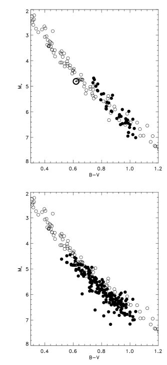
Figure 7: The sample of long-lived stars separated into 2 parts. Plot (a) shows the Hyades sequence (open symbols) and the 40 stars in the sample that have [Fe/H]$>$+0.14, which is the metallicity of the Hyades [Perryman et al., 1998], plot (b) shows stars with [Fe/H]$<$+0.14. The Hyades stars have been selected by [Perryman et al., 1998] as single stars within 10 pc of the cluster centre. The sun is located at (0.62, 4.81). These figures clearly illustrate the existence of a large proportion of metal-rich stars in the sample.

3 Comparison with previous metallicity distributions

3.1 General comments

Different biases may affect the metallicity distribution due to selection criteria of the observed stars. Two such biases have been discussed and corrected in the previous section. In the literature, only the first one has been corrected (the age bias), although it is the least important one. An even more problematic bias occurs prior to the two former biases mentioned, in samples selected on the basis of spectral type. A selection on spectral type is sometimes imposed by the availability of photometric surveys (such as Strömgren surveys of Olsen), but seems to be perpetuated for rather historical reasons (the ‘G-dwarf’ metallicity distribution) than real limitations in the available data. Unfortunately, spectral type criteria introduce biases in the metallicity distribution which are almost impossible to correct.

We have demonstrated in section 2.3.2 how the colour limit of the observed samples introduces a non-negligible bias against metal-rich stars. In order to be able to correct this bias, one must know the colour limits of the sample. This is impossible to obtain once the selection has been made from spectral type, due to the intrinsic high dispersion of colours at a given spectral type. A brief inspection of the Third edition of the Catalogue of Nearby Stars (hereafter CNS3, [Gliese & Jahreiß, 1991]) illustrates this point: for example G5 V stars have colours extending from $B-V$=0.58 to 1.1. and G0 V stars from 0.50 to 0.69. The intricacy of colours between spectral types forbids a clean definition of the sample mass limits.

The metallicity bias introduced is even more severe if one does not include sufficiently late spectral types. This point has been discussed in [Grenon, 1978], [Grenon, 1987]. According to [Grenon, 1990], turn-off of the oldest solar metallicity stars is $B-V$=0.68, which implies that samples selected on spectral types earlier than G2 V or G5 V would miss most of them, not to speak of metal-rich stars. We show below that an unbiased sample must comprise spectral type as late as K.

In the last five years numerous studies of the local metallicity distribution of dwarfs have been published [Wyse & Gilmore, 1995, Rocha-Pinto & Maciel, 1996, Flynn & Morell, 1997, Favata et al., 1997, Rocha-Pinto & Maciel, 1998]. All are based on trigonometric distances from the CNS3 or CNS2. The first two and [Rocha-Pinto & Maciel, 1998] used Strömgren photometry, while Flynn & Morel designed their own metallicity indicator based on the $B_{1}$ Geneva and the $R-I$ Cousins colour indices. Finally [Favata et al., 1997] relied on their own spectroscopic determinations. As a general rule, it can be said that the metallicity distributions of all these authors present the same characteristics. Briefly : a broad maximum is found between [Fe/H]=$-0.3$ and $-0.1$, 20–30 percent of the stars have [Fe/H]$>$0.0, 10 to 20 per cent between -1.0$<$[Fe/H]$<$-0.5. Very few or no stars have [Fe/H]$<$-1 (however Flynn & Morel find 7 stars with [Fe/H]$<$-1.0) or [Fe/H]$>$0.3. The exception to this rule is [Favata et al., 1997], with a distribution that peaks at a somewhat higher metallicity than the others with the consequence that 41 per cent of their stars have a metallicity higher than solar, and 7 per cent between -1.0$<$[Fe/H]$<$-0.5.

In order to understand the origin of the differences and similarities between our metallicity distribution and those obtained by [Wyse & Gilmore, 1995, Rocha-Pinto & Maciel, 1996, Favata et al., 1997], we examine in more detail the samples used by these authors.

3.2 Comparison with other studies

[Wyse & Gilmore, 1995]

Out of 90 stars in the Wyse & Gilmore (1995) sample given as nearer than 30 pc in the CNS3 catalogue, 28 are in fact at a larger distance according to $Hipparcos$ parallaxes. The great majority of these were selected on the basis of trigonometric parallax in the CNS3 corresponding to a distance between 20 and 30 pc. All had large errors on parallaxes.

An interesting point is the presence of metal-rich stars in our sample which are totally absent from the sample by Wyse & Gilmore. This difference is an illustration of the bias introduced by spectral type. The sample of Wyse & Gilmore (1995) resulted from the cross-identification of the CNS3 and [Olsen, 1983] catalogue of Strömgren photometry for F/G0 spectral types. Wyse & Gilmore (1995) then applied a 2^nd selection by excluding stars outside the interval 0.4$<B-V<$0.9. A consequence of their spectral type selection is that 10 stars in our sample with [Fe/H]$>$ 0.2 and 0.4$<$ B-V $<$0.9 are absent from the Wyse & Gilmore (1995) sample. Nine of these objects are in the CNS3, but have G5V–K0V spectral types, and are therefore absent from the catalogue of [Olsen, 1983]. Even more surprising is the fact that for 39 stars with [Fe/H]$>$0 and $B-V<$0.9 in our sample, none has a (Simbad) spectral type earlier than G5. Therefore, 39 stars selected as long-lived objects and [Fe/H]$>$0 in our sample are absent from the sample of Wyse & Gilmore (1995).

Finally, note that due to the accurate $Hipparcos$ parallaxes, the overdensity of metal-poor stars found by Wyse & Gilmore (1995) is washed out. Fifteen stars ($\approx$ 6 per cent) have $[$M/H$]<$-0.5 in our sample, 17 (19 per cent) in Wyse & Gilmore (1995). Six stars only are in common. Nine stars in the sample of Wyse & Gilmore (1995) have a parallax smaller than 40 mas and have not been included in our sample. Two stars have a parallax larger than 40 mas but have a multiplicity flag in the $Hipparcos$ catalogue.

[Rocha-Pinto & Maciel, 1996]

[Rocha-Pinto & Maciel, 1996] have selected a sample similar to that of Wyse & Gilmore (1995), except that they extended their selection to all G dwarfs in the Gliese catalogue. Thus, they are less sensitive to bias against metal-rich stars (but see below): approximately 20 per cent of their sample has [Fe/H]$>$0. They find very few stars with [Fe/H]$>$0.2 (approximately 2 per cent), and their distribution peaks between [Fe/H]=-0.2 and -0.3. Several factors contribute to the importance of this peak. First note that 47 per cent of the stars are illegitimate in the sample of [Rocha-Pinto & Maciel, 1996], because of parallaxes smaller than 40 mas according to $Hipparcos$. Second, the use of [Schuster & Nissen, 1989] metallicity calibration underestimates the metallicity of the stars. Finally, the limitation to spectral types G is undoubtedly a source of bias, (even though it is less important than for the previous study). Fig. 8(a) shows their metallicity distribution, after cleaning from objects with $\pi_{Hipparcos}<40$ mas. We also removed those objects which are subgiants and giants according to their position in the HR diagram. The result is not very different from their initial distribution (see their Fig. 2).

On the same plot, we show our sample, from which we have removed all K-type stars, in order to mimic the selection of [Rocha-Pinto & Maciel, 1996]. The effect of this simple modification is to produce a new distribution which peaks at -0.3$<$[Fe/H]$<$-0.2, in agreement with that of [Rocha-Pinto & Maciel, 1996]. The bias is clear : by simply removing K-type stars, the sample is shifted from [Fe/H]$\approx$0.0 to -0.3$<$[Fe/H]$<$-0.2

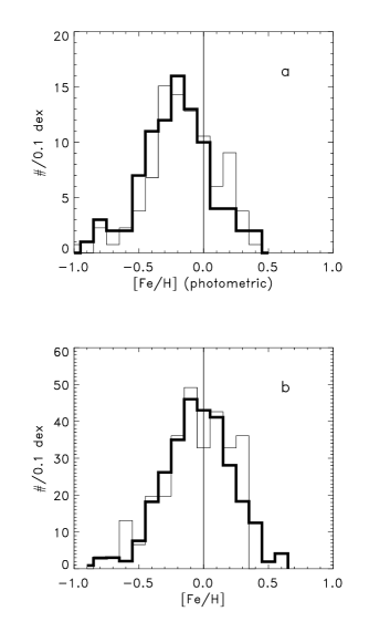
Figure 8: Plot (a) illustrates how a bias against metal-rich stars is introduced by selecting G-type stars. The plot shows our sample of long-lived dwarfs, with all K-type stars removed, to mimic the metallicity bias (in thick line). The sample of [Rocha-Pinto & Maciel, 1996], which contains only G-type stars (cleaned using $Hipparcos$ parallaxes) is also shown. The lower plot shows our distribution (all stars, corrected as described in section 2) and the distribution by [Favata et al., 1997], which shows no apparent bias. Histograms have been normalised to contain the same number of stars.

[Favata et al., 1997]

The distribution obtained by Favata et al. is interesting because (1) it is based on spectroscopic measurements and (2) its maximum is shifted towards solar metallicity stars, as in our sample. They have measured the iron abundance for 91 stars among the 1979 edition of the catalogue of Nearby stars (Gliese & Jahreiss, 1979), limited to stars with $\pi>$ 0.045$\arcsec$. The distance definition of the sample suffers from problems mentioned for previous samples, with 40 per cent of these 91 stars being outside the 22.5 pc sphere. However, although the sample is obviously incomplete in distance, it is probably not biased by spectral type because the objects were selected at random in a given colour interval. The result on Fig. 8(b) is a distribution very similar to that of our sample.

Conclusions

Examination of the first two examples shows that they certainly suffer from biases introduced by a selection on spectral types. Although the attention in the literature has been mainly focused on biases affecting low metallicity stars, we argue that at least as much important biases have truncated the metal-rich ([Fe/H]$>$0) side of the metallicity distribution. All three samples are plagued by incompleteness of the colour intervals and underestimated distances from the Catalogue of Nearby Stars. As a conclusion, we should say that the two studies by [Rocha-Pinto & Maciel, 1996] and Wyse & Gilmore (1995) have provided G dwarf metallicity distributions consistent with each other. However, G dwarfs are not representative of the metallicity of the disc, and are biased against metal-rich stars. On the contrary, when the samples are not limited to G spectral types, as is the case for [Favata et al., 1997], the metallicity distribution contains about 40 per cent of stars with [Fe/H]$>$0.0.

3.3 A glimpse on the age distribution of the sample

In models describing the chemical evolution of the galactic disc with infall, the infall rate fixes the pace at which the galactic disc is built, through the SFR. This is well illustrated in models reviewed by Tosi (1996). Because the infall rate is usually taken as a decreasing function of time, the SFR history follows. Thus, since infall is so widely used to explain the lack of metal-poor dwarfs observed in the solar neighbourhood, a desirable test of these models would be the age distribution of dwarfs that make the metallicity distribution. Unfortunately, as mentioned previously, most of the stars in the sample have a main sequence evolution that is too close to the ZAMS to have an age determined with some accuracy in the HR diagram. However, an interesting information is available for the young dwarfs because they can be detected as X-ray emitters due to coronal activity. The cross-identification between the $ROSAT$ survey and the Catalogue of Nearby Stars [Huensch et al., 1999] can be used to quantify the percentage of potentially young stars in our sample.

There are 90 stars (40 per cent) in our sample in the list of objects resulting from this cross-identification. Fig. 9(a) shows the X-ray flux of these stars as a function of $B-V$ colour. The figure shows that our sample may contain slightly over 90 stars with X-ray luminosity brighter than log X/L_bol=-5.5, which could be absent from the sample of Huensch et al. (1999), due to the incompleteness to the X-ray data for the reddest stars. In order to get a rough estimate the corresponding ages, we utilise the log L_X/L_bol-logR’_HK relation of Sterzik & Schmitt (1997) and the logR’_HK-logt relation of Soderblom et al. (1991). According to these relations, log L_X/L_bol=-5.5 corresponds to an age of 2 Gyr. Most our stars having X-ray emission at the level of log L_X/L${}_{bol}>$-5.5 could therefore be considered younger than 2 Gyr.

Fig. 9(b) illustrates what the metallicity distribution of these stars is. It is centred on [Fe/H]=0.0, with an unexpected but important contribution of 11 stars with [Fe/H]$<$-0.3. Some of these stars have a spectroscopic iron abundance which confirms the photometric iron abundance. For instance, HIP 88622 has [Fe/H]_photo=-0.506, and [Fe/H]_spectro=-0.47, dated 15 Gyr in [Edvardsson et al., 1993], and HIP 15510 has [Fe/H]_photo=-0.35, and [Fe/H]_spectro=-0.48 [Pasquini et al., 1994]. The X-ray emission of HIP 88622 may appear somewhat puzzling because of its metallicity, and because HIP 88622 has no significant chromospheric emission according to Pasquini et al. (1994). While these cases may be exceptions, it has been suggested more generally that activity may affect photometric indices and that presumably young stars may be measured as deficient objects if abundance is measured from photometry [Gimenez et al., 1991, Morale et al., 1996, Favata et al., 1997, Rocha-Pinto & Maciel, 1998]. This effect may explain the shape of the histogram of Fig.9, but its importance is uncertain, and we do not try to correct it. While some of the stars may have been detected as X-ray emitters in the sample for reasons not related to their age, it is clearly demonstrated that X-ray emission is a tracer of young stars [Guillout et al., 1998]. In this respect, the fact that around 40 per cent of the sample is composed of X-ray emitters that have ages less than 2 Gyr suggests a few comments.

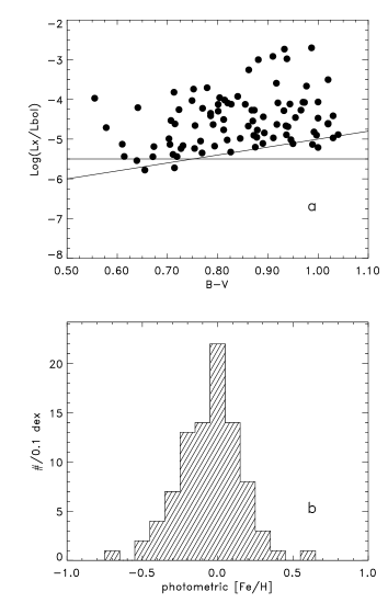
Figure 9: (a) X-ray flux as given in [Huensch et al., 1999] as a function of $B-V$ colour. The horizontal line shows approximate flux level for 2 Gyr stars according to the logL_X-logR’_HK relation of [Sterzik & Schmitt, 1997] and the logR’_HK-logt relation of [Soderblom et al., 1991]. The other line delineates the incompleteness of the X-ray data, according to [Sterzik & Schmitt, 1997]. The 90 stars may slightly underevaluate the number of X-ray emitters in our sample, because of incompleteness of the X-ray data $B-V>$0.8. (b) Photometric metallicity distribution of stars in (a).

In section 5, we calculate a model metallicity distribution assuming a constant SFR. We argue that although a constant SFR is not phenomenologically directly related to the gas content, it is compatible with available determination of the SFR history in the Milky Way. If a constant star formation rate has dominated the history of the galactic disc, then of the order of 15–25 per cent of the stars are expected to have an age less than 2 Gyr (for a 8-12 Gyr thin disc). However, a distance limited sample of the solar neighbourhood is biased against old stars because of the secular heating of the disc, observed in the increase of the vertical velocity dispersion with age. Using the correction factors introduced in section 5.2.2, (factor of 5 decrease in the surface density for stars between 8 and 4 Gyr, 2.2 for stars between 4 and 1 Gyr, normalised to 1 for stars with age less than 1 Gyr. The thin disc age is taken to be 8 Gyr; adopting 10 Gyr, this estimate changes to 40 per cent), we obtain of the order of 45 per cent of the local stellar material to have an age less than 2 Gyr. This is compatible with 40 percent of the stars having X-ray emission.

4 Final distribution

4.1 [Fe/H] distribution

As already mentioned, a distribution suitable for comparison with presently available chemical evolution models is the percentage of mass found at different metallicities. To obtain such distribution, we estimate the mass of each star from the adequate isochrone [Bertelli et al., 1994] – for unevolved stars – or evolutionary track – for those stars for which evolution is significant. The masses of unevolved stars have been estimated by matching the observed and theoretical absolute magnitudes on the isochrone. We have not taken the colour into account because of the uncertainty of the stellar model temperatures and the conversion to colour [Lebreton, 2000]. For this reason, it is expected that for some stars that fall below their isochrone, the mass may correspond to a colour on the isochrone that is beyond the colour limit at B-V=1.05 shown on Fig. 10a. Stars near the turn-off all fall within the limit, because the fit to the stellar models includes the age as a supplementary parameter. The resulting fraction of stellar mass as a function of metallicity is plotted on Fig. 10b.

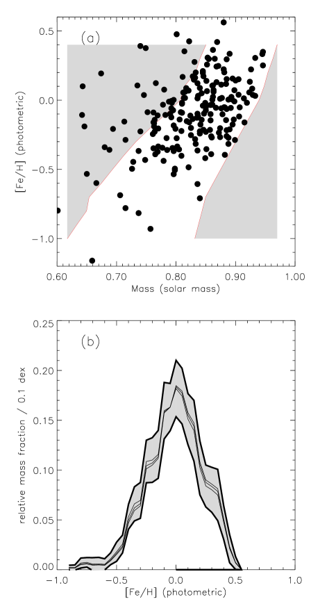
Figure 10: (a) : Mass-metallicity distribution for dwarfs in the sample. The 2 lines show the selections due to the colour limit at $B-V$=1.05 (left) and turn-off (right). The gray areas shows the limits within which a correction has been applied. (b) : the final metallicity distribution of stellar material in the solar neighbourhood. The result is illustrated adopting 3 different IMF slopes (0.05,0.7,1.2), which shows negligible effect (the 3 curves). The gray area shows the uncertainty in the distribution due to poisson noise.

Table 1: Percentage of stellar mass as a function of metallicity in the solar neighbourhood per 0.1 dex bin

[Fe/H]	%	error(%)
-0.90	0.23	0.22
-0.85	0.23	0.25
-0.80	0.68	0.50
-0.75	0.74	0.48
-0.70	0.57	0.64
-0.65	0.59	0.65
-0.60	0.54	0.56
-0.55	1.10	0.59
-0.50	1.80	0.96
-0.45	2.58	0.89
-0.40	5.31	1.25
-0.35	6.61	1.71
-0.30	6.96	1.80
-0.25	10.86	2.13
-0.20	11.01	2.24
-0.15	11.58	2.40
-0.10	15.96	2.83
-0.05	16.32	2.38
0.00	18.18	2.83
0.05	17.43	2.79
0.10	15.11	2.57
0.15	13.95	3.05
0.20	10.22	2.70
0.25	8.40	2.10
0.30	8.02	2.26
0.35	7.50	2.58
0.40	4.74	1.69
0.45	2.11	1.41
0.50	0.67	0.64

In order to correct for the bias introduced by the colour limit and the selection of long-lived objects, we use the following procedure. We assume a given initial mass function, the same at all metallicities over the mass interval of interest, from 0.60 to 0.95M_⊙. This IMF is used to extrapolate the amount of stellar mass outside the mass interval where completeness is achieved. The number of stars as a function of [Fe/H] within the mass interval where completeness is achieved is used as normalisation. The plot of fig. 10b shows the resulting metallicity distribution for different IMF slopes. The influence of the IMF slope is negligible, due to the small mass interval involved. We have also evaluated the contribution of the poisson noise to the distribution. If N stars in the sample contribute to a given metallicity interval $\Delta$[Fe/H], we can evaluate the total mass $\sqrt{N}$ stars would represent, weighted by the adopted IMF. The resulting distribution, together with its errors is given in Table 1.

4.2 [O/H] distribution

In order to have a distribution comparable with the predictions of the Simple Closed-Box model with instantaneous recycling approximation or other types of models which use the instantaneous approximation, the iron distribution is usually converted to an oxygen abundance distribution. Since Pagel (1989), this is achieved by noting that oxygen, being mostly synthesized in type II supernovae, whose recycling time is negligible, is better suited to compare with the Simple model. Clegg et al. (1981) have shown that [O/H]=0.52[Fe/H]+0.03 for -1$\leq$[Fe/H]$\leq$+0.4, which has subsequently been approximated to [O/H]=$0.5$[Fe/H] in studies dealing with the G-dwarf metallicity distribution. Applying this relation to the [Fe/H] distribution much strengthens the narrowness of the distribution and the disagreement with the SCB model, and it deserves more attention. There is now a large debate on the exact behavior of the [O/Fe] ratio as a function of [Fe/H] for [Fe/H]$<$-1.0. We are interested here in the metal-richer part at [Fe/H]$>$-1.0.

When measured on the dataset by Edvardsson et al. (1993), a linear regression yields

$$[O/H]=$0.64$*[Fe/H]-0.041$$ (3)

while the study by [Carretta, Gratton, & SnedenCarretta et al., 2000] gives the relation

$$[O/H]=$0.51$*[Fe/H]-0.064$$ (4)

and the study by [Chen et al., 2000] gives the relation

$$[O/H]=$0.70$*[Fe/H]+0.07$$ (5)

The difference of 0.11 dex offset between the relations 3 and 5 is due to different temperature scales adopted in the two studies, as mentioned by Chen et al. (2000). In the metallicity range of interest, the second relation gives similar results to the relation of Clegg et al. (1981), implying a narrow [O/H] distribution, but with a shift of 0.1 dex. On the contrary, the relation of Chen et al. (2000) seriously reduces the effect of converting from [Fe/H] to [O/H]. Looking at Fig 11, it seems that the conversion to [O/H] comes as an additional uncertainty in an already long list of approximations whose effect has not been seriously accounted for. There are too few indications that can help us deciding which conversion to apply, hence, we prefer to keep on working with the [Fe/H] distribution.

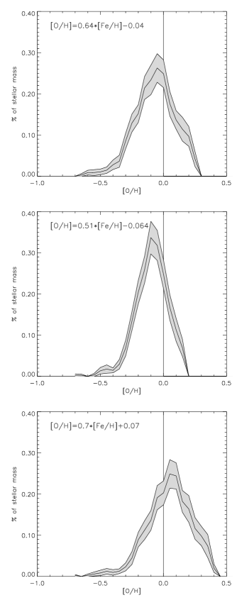
Figure 11: Distribution of stellar mass with [O/H], adopting 3 different [Fe/H] to [O/H] relations from [Edvardsson et al., 1993] (a), [Carretta, Gratton, & SnedenCarretta et al., 2000] (b), [Chen et al., 2000] (c).

5 The Simple Closed-Box model

Two kinds of assumptions define the Simple Closed-Box model. The first kind assumes that complex physical processes can reasonably be represented by simple analytical laws. They reflect our (poor) knowledge of these processes but are convenient for the derivation of the model results. These assumptions include : (1) an IMF constant with time, (2) no exchange of matter (3) the interstellar medium is initially free of metals (4) the interstellar medium is homogeneous at all times. Assumptions of the second kind are introduced purely for analytical tractability. This is the case for the instantaneous recycling approximation (IRA). We are tempted to classify assumption (4) in the second category, because it is possible to conceive sub-SCB models which would evolve independantly at slightly different rates and that would preserve individually the characteristics of the SCB model. This would give rise to some amount of inhomogeneity in the metallicity distribution without corrupting the Simple model as the main evolutionary path for chemical evolution.

5.1 The ‘G-dwarf problem’ : A little bit of semantics

The ‘G-dwarf problem’ is usually referred to as the lack of metal-poor stars in the vicinity of the sun, relative to the SCB model. However, the ‘G-dwarf problem’ seems to cover two different problems. In Section 3, we have demonstrated that there is a real ‘G-dwarf’ problem in the sense that a sample of G-dwarf stars is inherently biased in regard to metallicity, and cannot be compared directly to chemical evolution models. Perhaps the ‘G-dwarf problem’ should more appropriately only refer to this specific bias.

The second aspect of the so-called G-dwarf problem (which arguably should better be quoted as the SCB model problem), refers to the long-lasting difference between the amount of metal-poor material generated by the SCB model, and the observed metallicity distribution.

5.2 Model input parameters

The derivation of the metallicity distribution of the stellar material in the case of the SCB model with IRA can be made analytically, due to the assumptions of the model, see for example [Binney & Tremaine, 1987]. In the case of zero initial metallicity of the gas in the disc, the metallicity evolves as

$$Z(t)=-p\-ln[S_{gas}(t)/S_{gas}(0)]$$ (6)

where S(0) is the initial gas surface density, and S(t) is the gas surface density at time t.

In the above equation, the yield p modulates the position of the peak of the metallicity distribution, and S(t) is an implicit combination of the SFR consumption of gas and the rejection rate of the stars. It is usually chosen so that the final ratio S_gas(t)/S_gas(0) meets the (loose) observational constraints of the solar neighbourhood. When the instantaneous approximation is not assumed, the gas fraction evolves as the complex result of stellar ejecta, lifetimes, and gas definitively locked up in low mass stars and stellar remnants. The resulting metallicity distribution is a function of the yield and the gas fraction of the disc, while the comparison with the data also depends on the disc thickening. We review each of these three points in turn.

5.2.1 The yield

The yield of a generation of stars is the mass of metals synthetized and ejected per unit mass of material locked for a sufficiently long time in stars and stellar remmants. It is dependant on nucleosynthesis, mass loss rate and stellar ejecta, but also on the IMF. In the case of the SCB model with IRA, the yield is chosen so that the equation above is compatible with the present fraction of gas in the disc and abundance of the interstellar medium. The abundance of the interstellar medium is usually evaluated to be solar [Binney & Merrifield, 1998] (this parameter is however very uncertain, and not necessarily representative of the evolution on the last Gyr. ). The gas fraction is situated between 0.1-0.3, depending on the adopted gas density (6–11M_⊙.pc^-2) and total density (40–50M_⊙.pc^-2). With these values and equation 6, the yield is evaluated to be within the range 0.0086-0.025, which is a fairly large range, and is of little help in defining the paramaters of the SCB model with IRA.

How does this estimate compare with the yield calculated from the local IMF and stellar yields ? Such yields have been calculated using a model with the following characteristics : The gas is ejected from stars assuming the same initial to final mass relation as that used in Scully et al. (1997), which comes from Iben & Tutukov (1984) :

m$\leq$6.8M_⊙   M_R=0.11$\times$m+0.45 M_⊙

m$>$6.8M_⊙   M_R=1.5M_⊙.

The stellar yields come from Portinari & Chiosi (1999) for massive stars and van den Hoek & Groenewegen (1997) for intermediate mass stars.

Although the IMF of solar neighbourhood stars is still highly uncertain, it is now admitted that it has at least two different regimes, for low (roughly lower than one solar mass), and high masses. The IMF at low masses is essential, but in many cases in the literature the value of the index adopted in chemical evolution models seems unrealistic. For instance, Portinari & Chiosi (1999) adopt x=1.35 for M$<$ 2 M_⊙, while others Gratton et al. (2000) use Scalo (1986), which is also too steep at low masses. Other works utilise a single index for calculating the yield, such as Pilyugin & Edmunds (1996). Recent measurements of the IMF from the solar neighbourhood luminosity function have proved that the IMF index at low masses is much shallower than the Salpeter value, at x=0.05 [Reid et al., 1996]. At higher masses, the IMF is much more uncertain (see Scalo (1998), Haywood et al. (1997b) for a review). We consider that values between x=1 and 2 are reasonable, and values between 2 and 3 are not unrealistic.

Figure 12: Yield weighted by the IMF as a function of the IMF slope for low mass stars ($<1$M_⊙) and high mass stars ($>$1M_⊙). The yield is calculated assuming stellar yields at solar metallicity, with specifications mentioned in the text.

Fig. 12 shows that for values of the high mass IMF index less than $\approx$ 1.9, the yield is larger than 0.01. For Salpeter IMF index, values of the yield as high as 0.05 are possible.

Assuming that the present ratio S_gas(t)/S_gas(0) is around 0.1–0.3 and that the abundance of the interstellar medium is of the order 0.02–0.03, this value is in the range of possible yields.

5.2.2 Surface and volume densities

An important issue when discussing the distribution of metallicities is the surface densities of the stellar and gas components in the solar neighbourhood. According to [Jahreiss & Wielen, 1997], the local stellar density is 3.9$\times$10^-2M_⊙.pc^-3. The projection to distance outside the galactic plane can be made assuming exponential density for the thin disc and the thick disc. Assuming the thick disc is responsible for 2 per cent of the local stellar mass, and has a scale height of 1400 pc [Reid & Majewski, 1993], the thin disc with 325 pc, then the relative amount of thick disc is of the order of 8–9 per cent. The total surface density of visible stars (i.e no stellar remnants) is of the order of 27 M_⊙.pc^-2. Taking into account the gas surface density and allowing for some stellar remnant, the total surface density is of the order of 40–50 M_⊙.pc^-2. Assuming disc characteristics as those proposed by [Haywood et al., 1997] and [Robin et al., 1996], one finds that the thick disc represents 15 per cent of the local stellar surface density.

A correlated problem is the correction one has to apply in order to convert volume densities to surface densities, and vice versa. This is a difficult problem, because the scale heights of the (thin and thick) discs are a function of age, which is not a quantity that can be derived for stars in the sample. Various attempts have been made, see in particular Sommer-Larsen (1991) and Wyse & Gilmore (1995). Wyse & Gilmore (1995) estimated a correction function of the metallicity. One problem with their solution is that they use the same correction for stars in the interval [Fe/H]=[-0.3,+0.3]. However, even though this may seem a rather narrow range, there is a significant age trend over this interval (see the age-metallicity relation below). It implies that such stars may have quite different ages, hence quite different correction should be applied. We choose to ‘correct’ the predicted distribution instead (that is, we convert model surface density to volume density), since metallicity is an explicit function of age in the model. This solution has the advantage of being consistent with the fact that the vertical velocity dispersion is also a known function of age.

Quantitative estimates of the corrections as a function of age have been derived using the oscillation period given in Wyse & Gilmore (1995). We combine this relative oscillation period with the age-vertical velocity dispersion relation given in Gómez et al. (2001). The combination of these two factors gives a relative correction of the order of 13 for ’thick disc’ stars, and 5 for the oldest disc stars. Note that these values are much larger than that applied by Wyse & Gilmore (1995), and partly explains why we succeed in giving a reasonable fit to the data. Note also that these values are compatible with scale height variations within the (thick and thin) disc.

5.3 Local constraints on the Simple Closed-Box model with no IRA

Since the previous section shows the uncertainty introduced by converting [Fe/H] to [O/H], we preferentially work with the iron distribution. This means that we have to drop the IRA and calculate numerically the metallicity distribution.

5.3.1 The model

The main characteristics of the model are given in Table 2. The stellar yields are used as described in section 5.2 for massive and intermediate mass stars. The stellar lifetimes come from [Pols et al., 1997], and are dependent on metallicity. The onset of type Ia supernovae happens when the metallicity reaches [Fe/H]=-1.0. The yields for the different species produced by type Ia SN are from Nomoto et al. (1984) (iron $\approx$ 0.6 M_⊙/event) and the rate of SNIa is assumed to be proportional to the number of SNII, with SNII/SNIa=8.5. Note that we don’t use a Schmidt law type SFR. While there are some evidences that the SFR of massive stars may be proportional to some power of the gas density, there are few evidences that this can be extrapolated to low and intermediate mass stars. Since determinations to date are compatible with a constant SFR history for the disc of the Milky Way, we use this simple prescription.

5.3.2 Metallicity distribution

The delayed ejection of important quantities of gas from long-lived stars could enhanced the dilution of metals in the interstellar medium, and permit the production of more stars at intermediate (e.g solar) abundance. In our tests however, this effect proved to be very minor, for the reason that the release of gas is spread on long time-scale by the important variation of stellar lifetime with abundance and mass; therefore, there is no sudden release of gas, and the dilution of metals in the interstellar medium is smoothed over long time scales.

The only marked effect of the SCB model with no IRA is the more rapid metallicity increase at the onset of SNIa at [Fe/H]=-1. This translates in the metallicity distribution into a shift of the distribution to higher metallicities, as can be seen at [Fe/H]$\approx$-1 (Fig.13a). The SCB with no IRA doesn’t seems to generate more solar metallicity stars. Note that this somewhat contradicts the findings of Scully et al. (1997). However, they use very different prescriptions (stellar lifetimes independent of metallicity, IMF index=1.7 over the whole mass range, which they take to be 0.4$\leq$ m/M_⊙ $\leq$ 100).

Table 2: Characteristics of the SCB model of Fig.15.

Surface density	40M⊙.pc-2
Initial metallicity	Fe/H=0.
SFR	Constant 3.5M⊙.pc-2.Gyr-1
IMF	x=0.05 m$<$ 1M⊙, x=1.7 m$>$ 1M⊙
Final gas density	8M⊙.pc-2
Age of the model	14 Gyr

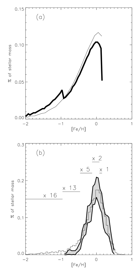
Figure 13: Plot (a) shows two Closed-Box models, one with IRA and yield p=0.02 (thin line) and no IRA (thick line), as described in the text. Plot (b) shows the SCB model (no IRA), converted to volume density as described in section 5.2.2, to which we have added a dispersion of 0.1 dex to account for metallicity measurement dispersion in the observed distribution.

The total duration of the model is 14 Gyr. In the model, we identify three phases corresponding (not necessarily in a univocal correspondance) more or less to the galactic stellar populations. The first phase is defined by [Fe/H]$<$-1.0 dex. We do not try to ascribe a particular stellar population (halo or thick disc) to this phase, and the scale height correction attributed to this metallicity range is arbitrary. In other words, we don’t include this part of the distribution in our discussion of the SCB model. This conservative position is justified to some extent by (1) the fact that the characteristics of the metal weak thick disc (or flattened halo ?) are still essentially unknown (2) the limited volume of our sample is not well suited for studying an intrinsically rare population. In the model, the duration of this phase is 3 Gyr. The thick disc phase starts at [Fe/H]=-1.0, and may last 2 to 3 Gyr, ending when the metallicity reaches -0.58 or -0.45. Then the thin disc phase may be identified with the remaining evolution, with the metallicity rising from -0.58 or -0.48 to [Fe/H]=+0.17. The disc as a whole is characterised by having around 11 Gyr, and a metallicity that evolves from [Fe/H]=-1 to [Fe/H]=+0.17.

Figure 13(b) shows the metallicity distribution of the SCB model with no IRA after the disc thickening has been accounted for. A gaussian noise of 0.15 dex has been added to account for metallicity dispersion at all ages, plus 0.1 dex for simulating individual measurement error. The figure shows a quite reasonable agreement between the model and the observations.

5.3.3 The age-metallicity relation

On Fig. 14(a), we display the age-metallicity relation (AMR) of the model, together with the one derived by [Rocha-Pinto et al., 2000]. The plot shows a reasonable agreement between the two over a large age range. Note that the two points corresponding to very old stars are upper limits according to [Rocha-Pinto et al., 2000].

The age-metallicity relation has been the subject of numerous studies since the work of [Edvardsson et al., 1993]. Because the cosmic dispersion in the relation is viewed as an important constraint for chemical evolution models, it has focused a number of comments (see [Rocha-Pinto et al., 2000] for a review). The dispersion in the AMR measured by [Edvardsson et al., 1993] is about 0.2 dex, larger than the one given by more recent studies. [Edvardsson et al., 1993] cautioned however that their sample has been chosen for representativeness of all metallicities, which doesn’t mean completeness at all metallicities. This makes their sample ill-suited for a correct measurement of the real dispersion. Although they provide corrections for the bias, their procedure is necessarily uncertain. It is not surprising that [Garnett & Kobulnicky, 2000] and [Rocha-Pinto et al., 2000] find a smaller dispersion, of the order of 0.10–0.15 dex. A consequence on the AMR is that the correlation between age and metallicity is tighter than has been thought after [Edvardsson et al., 1993]. This view confirms that the distinction made (section 5.2) in the scale height corrections for stars with metallicity varying between -0.5 and +0.2 is justified.

There are three main processes by which the dispersion may be explained: inhomogeneity in the interstellar medium [Malinie et al., 1993], diffusion of stellar orbits [Grenon, 1987, Francois & Matteucci, 1993, Wielen et al., 1996], and sporadic infall [van den Hoek & de Jong, 1997]. While it is almost certain that the first two play a role, even if minor, infall has the capability to explain large dispersion in the age-metallicity relation.

Whatever the processes that lead to variations of the conditions of the star birth, it is worth noting that a 10 per cent dispersion on the IMF, SFR and SN1 rate is sufficient to account for the observed dispersion. This is illustrated in Fig.14a), where each point has been simulated as the result of SCB models with slightly different properties simulated at random from the model of table 2 allowing for 10 percent dispersion in the IMF slope (for m$>$ 1M_⊙), SNIa rate and SFR. A weighting according to the disc thickening described in section 5.2.2 has been applied. Fig. 14b shows the metallicity histogram for these simulated points, compared to the metallicity distribution of Fig. 6.

Figure 14: (a) The mean age-metallicity relation given by the model (thick curve). The dots are calculated according to the same model, but assuming 10 per cent dispersion on the IMF, SFR, and SN1 rate, plus 0.1 dex ‘measurement error’ in [Fe/H] and age. This simulated ‘local’ distribution has been weighted according to the disc thickening described in section 5.2.2. The points with error bars are the observed age-metallicity relation according to [Rocha-Pinto et al., 2000]. Note that the two points corresponding to ages 11.5 and 13.5 Gyr are only upper estimates. (b) Shows the histogram of metallicities for these points (thick line). The histogram of Fig. 6 is also shown (thin line).

5.3.4 Abundance ratios

Our aim here is to demonstrate further how a model with simple prescriptions gives a satisfactory fit to complementary local constraints such as abundance ratios.

Fig.15 displays these ratios for CNO and Si, Mg elements. The model has obvious failures (N/Fe, Mg/Fe) and reasonable success (O/Fe, C/Fe), in comparable proportion to more sophisticated models [Timmes et al., 1995, Portinari et al., 1998, Goswami & Prantzos, 2000]. Possible reasons for the failure of N/Fe, Mg/Fe are discussed in [Goswami & Prantzos, 2000], and we don’t replicate their discussion.

Figure 15: Abundance ratios for Carbon, Nitrogen, Oxygen, Silicon and Magnesium.

6 Discussion

A reanalysis of the solar neighbourhood metallicity distribution has brought the following results :

(1) The metallicity distribution of long-lived dwarfs is centred on [Fe/H]$\approx$0, not [-0.3,-0.1]. When considering a sample of stars with no bias on the age, between 40 and 50 percent of stars have metallicity higher than [Fe/H]=0. Most previous studies have used samples biased against stars with solar metallicity or higher. This result reconciles the age-metallicity relation with the dwarf metallicity distribution.

(2) The percentage of mid-metal-poor stars ([Fe/H]$<$-0.5) is in agreement with estimates of the thick disc density from remote star counts and is situated between 2-4 per cent. The thin disc is not an important contributor to stars with [Fe/H]$<$-0.5.

(3) 40 per cent of these long-lived stars in our sample are X-ray emitters, which suggest that a large part of the sample may consist of young stars (age $<$2 Gyr). This supports the idea that the SFR is not a decreasing function of time.

(4) We have evaluated the distribution of stellar mass with metallicity. Due to selection criteria of observed samples, stars of varying metallicities are sampled on unequal mass intervals. We show that if this effect is left uncorrected, a second important bias against metal-rich stellar mass is introduced.

(5) We argue that a reasonable fit to the [Fe/H] distribution can be obtained with a SCB model with no instantaneous recycling approximation. Satisfactory fits are also obtained for the age-metallicity relation and abundance ratios. These results suggest that the solar neighbourhood metallicity distribution contains few (or no) indications that long time-scale infall may have play a major role in the building of the galactic disc.

In their study, Wyse & Gilmore (1995) commented that ‘even were the Simple Box model to fit some dataset, its inherent implausibility means that it is more likely that several compensating effects had generated this agreement by chance’. How much unrealistic is the SCB model presented here ? Our model incorporates all ingredients usually found in chemical evolution models of the Galaxy, (i.e metallicity-dependent stellar yields and lifetimes, empirical IMF and SFR), and satisfies local constraints. The only marked feature absent in our model is infall. While infall is prevalent in chemical evolution models, it is merely viewed as an additional free parameter to control the dilution of metals in the interstellar medium. In this respect, the SCB model is as much realistic as other models, but it is simpler. However, the remark of Wyse & Gilmore (1995) still holds, and the assumptions of the SCB models should be looked at with even more scrutiny.

The SCB model is basically a description of the chemical evolution of the mean parameters of the galactic disc. What we seek in fitting the observed distribution presented here is to know if the evolutionary path followed by the SCB model is the correct one. This approach has a chance of being sound if the assumptions of the SCB models do not contradict observed features. We shortly review the main assumptions of the SCB model.

(1) Initial metallicity Fe/H=0. It was not necessary to adopt a non-zero initial metallicity to account for the observed metallicity distribution. If correct, this implies that stars at arbitrarily low metallicities with disc kinematics must exist. Morrison et al. (1990) found that thick disc stars possibly reach as low metallicities as [Fe/H]=-1.60, while Martin & Morrison (1998) have been able to show that objects with thick disc kinematics can reach [Fe/H]=-2.05. It remains to be demonstrated that thick disc metallicities can reach even lower values. Note that at the same time, [Fuhrmann, 1998] showed that the halo and thick disc may be contemporary.

(2) Constant IMF. There is to date no clear-cut evidence for systematic variations in the IMF. The case for a universal IMF has been considered by different authors (Kroupa, astro-ph/0009005; Gilmore (1999)) and is favored at low masses ($<$1M_⊙). The diagnostic for a universal IMF is much less clear for masses of concern in nucleosynthesis [Scalo, 1998]. Variable IMF have been envisaged in the context of chemical evolution but has received relatively poor support (e.g Martinelli & Matteucci (2000) and Chiappini et al. (2000) for recent attempts).

(3) Homogeneous interstellar medium. As mentioned above, this is a minor assumption of the SCB model, introduced for analytical tractability. Inhomogenity can be introduced in the model while keeping with the SCB model as the main evolutionary path for chemical evolution. For example, it may be conceived that the disc as a whole has behaved as an ensemble of sub-SCB models with slightly varying properties. This would not seriously affect the picture of the SCB model as the progressive enrichment of a gaseous disc initially free of metals.

(4) Closed Box. This arguably is the most challenging hypothesis of the SCB model. Note that what we have assumed with this hypothesis is that the surface density of the model has remained constant, therefore fixing the rate of dilution of metals. In sophisticated models where the Closed-Box hypothesis is not assumed, infall is essentially viewed as a way to regulate the metal enrichment, in order to provide a solution to fitting the observed metallicity distribution. It works essentially as an additional free parameter. In view of the work presented here, infall looks unnecessary to describe the solar vicinity metallicity distribution. The local fossil signature of infall is still to be found. We note that the potentially most serious indication that infall processes may have played an important role in the building of the disc lies in the age-metallicity relation.

Infall provides the only mechanism to generate old metal-rich (solar-like) stars at the solar radius. If it can be demonstrated that old stars (age$>$8 Gyr) with disc-like kinematics and solar-like abundance exist in significant proportion, then they may represent the signature that the disc, or part of the (old) disc has formed through an evolutionary path that differs from the SCB model evolution.

References

- [Alonso et al., 1996] Alonso A., Arribas S., Martinez-Roger C., 1996, Astronomy and Astrophysics Supplement Series, 117, 227
- [Axer et al., 1995] Axer M., Fuhrmann K., Gehren T., 1995, Astron. Astrophys., 300, 751
- [Bertelli et al., 1994] Bertelli G., Bressan A., Chiosi C., Fagotto F., Nasi E., 1994, Astronomy and Astrophysics Supplement Series, 106, 275
- [Binney et al., 2000] Binney J., Dehnen W., Bertelli G., 2000, Mon. Not. R. Astron. Soc., 318, 658
- [Binney & Merrifield, 1998] Binney J., Merrifield M., 1998, ”Galactic astronomy”. Galactic astronomy / James Binney and Michael Merrifield. Princeton University Press. (Princeton series in astrophysics)
- [Binney & Tremaine, 1987] Binney J., Tremaine S., 1987, ”Galactic dynamics”. Princeton, NJ, Princeton University Press, 1987, 747 p.
- [Brinchmann & Ellis, 2000] Brinchmann J., Ellis R. S., 2000, Astrophys. J., Lett., 536, L77
- [Carretta, Gratton, & SnedenCarretta et al., 2000] Carretta E., Gratton R. G., Sneden C., 2000, Astron. Astrophys., 356, 238
- [Castro et al., 1997] Castro S., Rich R. M., Grenon M., Barbuy B., McCarthy J. K., 1997, Astron. J., 114, 376
- [Cayrel De Strobel et al., 1997] Cayrel De Strobel G., Soubiran C., Friel E. D., Ralite N., Francois P., 1997, Astronomy and Astrophysics Supplement Series, 124, 299, Provided by the NASA Astrophysics Data System
- [Chen et al., 2000] Chen Y. Q., Nissen P. E., Zhao G., Zhang H. W., Benoni T., 2000, Astron. Astrophys. Suppl. Ser., 141, 491
- [Chiappini et al., 1997] Chiappini C., Matteucci F., Gratton R., 1997, Astrophys. J., 477, 765
- [Chiappini et al., 2000] Chiappini C., Matteucci F., Padoan P., 2000, Astrophys. J., 528, 711
- [Clegg et al., 1981] Clegg R. E. S., Tomkin J., Lambert D. L., 1981, Astrophys. J., 250, 262
- [Edvardsson et al., 1993] Edvardsson B., Andersen J., Gustafsson B., Lambert D. L., Nissen P. E., Tomkin J., 1993, Astron. Astrophys., 275, 101
- [Favata et al., 1997] Favata F., Micela G., Sciortino S., 1997, Astron. Astrophys., 323, 809
- [Favata et al., 1997] Favata F., Micela G., Sciortino S., Morale F., 1997, Astron. Astrophys., 324, 998
- [Feltzing & Gustafsson, 1998] Feltzing S., Gustafsson B., 1998, Astronomy and Astrophysics Supplement Series, 129, 237
- [Flynn & Morell, 1997] Flynn C., Morell O., 1997, Mon. Not. R. Astron. Soc., 286, 617
- [Francois & Matteucci, 1993] Francois P., Matteucci F., 1993, Astron. Astrophys., 280, 136
- [Fuhrmann, 1998] Fuhrmann K., 1998, Astron. Astrophys., 338, 161
- [Garnett & Kobulnicky, 2000] Garnett D. R., Kobulnicky H. A., 2000, Astrophys. J., 532, 1192
- [Gilmore, 1999] Gilmore G., 1999, in The Identification of Dark Matter, p. 121
- [Gimenez et al., 1991] Gimenez A., Reglero V., de Castro E., Fernandez-Figueroa M. J., 1991, Astron. Astrophys., 248, 563
- [Gliese & Jahreiß, 1991] Gliese W., Jahreiß H., 1991, Preliminary version of the third catalogue of nearby stars, Technical report
- [Goswami & Prantzos, 2000] Goswami A., Prantzos N., 2000, Astron. Astrophys., 359, 191
- [Gratton et al., 2000] Gratton R. G., Carretta E., Matteucci F., Sneden C., 2000, Astron. Astrophys., 358, 671
- [Grenon, 1978] Grenon M., 1978, Publications de l’Observatoire de Genève, 1
- [Grenon, 1987] Grenon M., 1987, Journal of Astrophysics and Astronomy, 8, 123
- [Grenon, 1990] Grenon M., 1990, in Proceedings of the Fifth IAP Workshop, Astrophysical Ages and Dating Methods, June 26-30, 1989., p. 153
- [Guillout et al., 1998] Guillout P., Sterzik M. F., Schmitt J. H. M. M., Motch C., Neuhaeuser R., 1998, Astron. Astrophys., 337, 113
- [Haywood et al., 1997] Haywood M., Robin A. C., Crézé M., 1997, Astron. Astrophys., 320, 440
- [Huensch et al., 1999] Huensch M., Schmitt J. H. M. M., Sterzik M. F., Voges W., 1999, Astron. Astrophys. Suppl. Ser., 135, 319
- [Iben & Tutukov, 1984] Iben I., Tutukov A. V., 1984, Astrophys. J., Suppl. Ser., 54, 335
- [Jahreiss & Wielen, 1997] Jahreiss H., Wielen R., 1997, Proceedings of the ESA Symposium ‘Hipparcos - Venice ’97’, 13-16 May, Venice, Italy, ESA SP-402 (July 1997), p. 675-680, 402, 675
- [Lebreton, 2000] Lebreton Y., 2000, Ann. Rev. Astron. Astrophys., 38
- [Malinie et al., 1993] Malinie G., Hartmann D. H., Clayton D. D., Mathews G. J., 1993, Astrophys. J., 413, 633
- [Martin & Morrison, 1998] Martin J. C., Morrison H. L., 1998, Astron. J., 116, 1724
- [Martinelli & Matteucci, 2000] Martinelli A., Matteucci F., 2000, Astron. Astrophys., 353, 269
- [Mermilliod et al., 1997] Mermilliod J. ., Mermilliod M., Hauck B., 1997, Astron. Astrophys. Suppl. Ser., 124, 349
- [Morale et al., 1996] Morale F., Micela G., Favata F., Sciortino S., 1996, Astron. Astrophys. Suppl. Ser., 119, 403
- [Morrison et al., 1990] Morrison H. L., Flynn C., Freeman K. C., 1990, Astron. J., 100, 1191
- [Olsen, 1983] Olsen E. H., 1983, Astron. Astrophys. Suppl. Ser., 54, 55
- [Pagel, 1989] Pagel B. E. J., 1989, in Evolutionary Phenomena in Galaxies, p. 201
- [Pasquini et al., 1994] Pasquini L., Liu Q., Pallavicini R., 1994, Astron. Astrophys., 287, 191
- [Perryman et al., 1998] Perryman M. A. C. et al., 1998, Astron. Astrophys., 331, 81
- [Pilyugin & Edmunds, 1996] Pilyugin L. S., Edmunds M. G., 1996, Astron. Astrophys., 313, 783
- [Pols et al., 1997] Pols O. R., Tout C. A., Schroder K., Eggleton P. P., Manners J., 1997, Mon. Not. R. Astron. Soc., 289, 869
- [Portinari & Chiosi, 1999] Portinari L., Chiosi C., 1999, Astron. Astrophys., 350, 827
- [Portinari et al., 1998] Portinari L., Chiosi C., Bressan A., 1998, Astron. Astrophys., 334, 505
- [Prantzos & Silk, 1998] Prantzos N., Silk J., 1998, Astrophys. J., 507, 229
- [Reid et al., 1996] Reid I. N., Hawley S. L., Gizis J. E., 1996, Astron. J., 111, 2469
- [Reid & Majewski, 1993] Reid N., Majewski S. R., 1993, Astrophys. J., 409, 635
- [Robin et al., 1996] Robin A., Haywood M., Crézé M., Ojha D., Bienayme O., 1996, Astron. Astrophys., 305, 125