Lyman Continuum Extinction by Dust in H ii Regions of Galaxies

Abstract

We examine Lyman continuum extinction (LCE) in H II regions by comparing infrared fluxes of 49 H II regions in the Galaxy, M31, M33, and the LMC with estimated production rates of Lyman continuum photons. A typical fraction of Lyman continuum photons that contribute to hydrogen ionization in the H II regions of three spiral galaxies is $\lesssim$ 50 %. The fraction may become smaller as the metallicity (or dust-to-gas ratio) increases. We examine the LCE effect on estimated star formation rates (SFR) of galaxies. The correction factor for the Galactic dust-to-gas ratio is 2-5.

1 Introduction

Dust grains exist everywhere — from circumstellar environment to interstellar space. Hence, radiation from celestial objects is always absorbed and scattered by dust grains. Without correction for the dust extinction, we inevitably underestimate the intrinsic intensity of the radiation, and our understanding of physics of these objects may be misled. Thus, dust extinction for nonionizing photons ($\lambda>912$ Å) in the interstellar medium (ISM) has been well studied to date (e.g., interstellar extinction curve: Savage & Mathis 1979; Seaton 1979; Calzetti, Kinney, & Storchi-Bergmann 1994; Gordon et al. 2000).

In H ii regions, Lyman continuum (LC) photons also suffer extinction by dust grains (e.g., Ishida & Kawajiri 1968; Harper & Low 1971). We refer to this another type of extinction as the Lyman continuum extinction (LCE). Indeed, the fraction of LC photons absorbed by dust in H ii regions can be large (e.g., Petrosian, Silk, & Field 1972; Panagia 1974; Mezger, Smith, & Churchwell 1974; Natta & Panagia 1976; Sarazin 1977; Smith, Biermann, & Mezger 1978; Aannestad 1989; Shields & Kennicutt 1995; Bottorff et al. 1998). Petrosian et al. (1972), for example, have estimated the fraction of LC photons contributing to hydrogen ionization to be 0.26 in the Orion nebula.

If a large amount of LC photons is absorbed by dust in H ii regions, the effect of the LCE on estimating the star formation rate (SFR) will be very large. This is because we can only estimate the number of ionizing photons, LC photons used for hydrogen ionization, from the observation of hydrogen recombination lines or thermal radio continuum. When we define the fraction of ionizing photons estimated from observations as $f$, we obtain

$$N^{\prime}_{\rm LC}=fN_{\rm LC}\,,$$ (1)

where $N_{\rm LC}$ and $N^{\prime}_{\rm LC}$ are the intrinsic and apparent production rates of LC photons, respectively. Unless we correct the observed data for the LCE, we cannot obtain the actual LC photon production rate, and then, the true SFR. Therefore, we should estimate the fraction, $f$, in H ii regions. However, the LCE has not been discussed in the context of estimating the SFR of galaxies before Inoue, Hirashita, & Kamaya (2001a, hereafter Paper I).

Paper I has proposed two independent methods for estimating $f$, and applied the methods to the Galactic H ii regions. Then, they have shown that there are a number of H ii regions with $f\lesssim 0.5$ in the Galaxy. Moreover, they have found that $f$ can be approximated to be only a function of dust-to-gas ratio. If the approximation can be applied to the nearby spiral galaxies and their observed dust-to-gas ratios are adopted, $f$ averaged over galactic scale is about 0.3. Therefore, the SFR corrected by the LCE effect is 3 times larger than the uncorrected SFR.

The aim of this paper is that we confirm these results of Paper I not only for H ii regions in our Galaxy but for extragalactic H ii regions. We also discuss if the effect of the LCE on estimating the SFR of galaxies is really important. We describe the method for estimating $f$ in section 2. Then, $f$ is determined for the H ii regions in the local group galaxies in section 3. We discuss the dependence of $f$ on the dust-to-gas ratio in section 4, and our conclusions are summarized in the final section.

2 Method for Estimating the Effect of LCE

To estimate $f$ in equation (1) for each H ii region, the apparent production rate of LC photons in each region, $N^{\prime}_{\rm LC}$, is compared to its IR luminosity, $L_{\rm IR}$. In this paper, we use a method for estimating $f$ presented in section 3 of Paper I.

According to equation (12) in Paper I, we obtain

$$f=\frac{0.44+0.56\epsilon}{0.28+5.6(L_{\rm IR,7}/N^{\prime}_{\rm LC,50})}\,,$$ (2)

where $\epsilon$ denotes the average efficiency of dust absorption for nonionizing ($\lambda>912$ Å) photons, and $L_{\rm IR,7}$ and $N^{\prime}_{\rm LC,50}$ are the IR luminosity and LC photon production rate normalized by $10^{7}$ $L_{\sun}$ and $10^{50}$ s^-1, respectively. The equation is based on the theory of the IR emission from H ii regions by Petrosian et al. (1972) and the following discussion by Inoue, Hirashita, & Kamaya (2000). It is also worthwhile to note that $L_{\rm IR,7}/N^{\prime}_{\rm LC,50}$ is proportional to the flux ratio of the IR emission to the thermal radio emission, H$\alpha$ line, etc. If we express in the form of the flux ratio, the determination of $f$ is free from the uncertainty of the distance to the object.

Here, we describe some assumptions adopted in the derivation of equation (2). Since $L_{\rm IR}$ is the total energy emitted by dust, the wavelength range is set to 8–1000 µm, which covers almost all wavelength range of dust emission. Also, it is supposed that the IR radiation from H ii regions is dominated by large ($\sim 0.1\micron$) grains in thermal equilibrium with ambient radiation field. In other words, we neglect the contribution to the total IR luminosity of very small grains ($\lesssim 0.01\micron$) and polycyclic aromatic hydrocarbons (PAHs), which emit mainly in the mid-infrared (MIR, 8–40 µm) (e.g., Dwek et al. 1997). In principle, the assumption would make us underestimate the total IR luminosity of dust in H ii regions because such MIR emission is observed from these regions (e.g., Pişmiş & Mampaso 1991; DeGioia-Eastwood 1992; Leisawitz et al. 1998). Fortunately, it seems that the contribution of the MIR luminosity to that of the total IR is enough small to be neglected (Figure 1 in Leisawitz et al. 1998). Thus, the IR spectral energy distribution (SED) of H ii regions is assumed to be a modified black-body function with one temperature through the paper.

Moreover, we do not take account of the existence of helium. This is because almost all (96% according to Mathis 1971) photons produced by helium recombination can ionize neutral hydrogen. We do not consider the escape of LC photons from H ii regions, either. Indeed, less than 3 % of LC photons can escape from the star-forming regions in nearby galaxies (Leitherer et al., 1995). In short, we deal with an ideal H ii region that consists of only hydrogen and dust, and where no LC photons leak.

Let us determine $\epsilon$, which denotes the average efficiency of dust absorption for nonionizing photons. The total (absorption and scattering) optical depth of dust, $\tau_{\lambda}$, is expressed by

$$\tau_{\lambda}=\frac{\tau^{\rm abs}_{\lambda}}{1-\omega_{\lambda}}=\frac{A_{\lambda}}{2.5\log e}\,,$$ (3)

where $\tau^{\rm abs}_{\lambda}$, $\omega_{\lambda}$, and $A_{\lambda}$ are the absorption optical depth of dust, the dust albedo, and the amount of extinction at wavelength, $\lambda$, respectively. We can determine $A_{\lambda}$ from an extinction curve, $X_{\lambda}$, and its normalization, $E_{B-V}$, i.e. $X_{\lambda}=A_{\lambda}/E_{B-V}$. The efficiency of dust absorption at wavelength, $\lambda$, $\epsilon_{\lambda}$ is defined as

$$\epsilon_{\lambda}\equiv 1-e^{-\tau^{\rm abs}_{\lambda}}=1-10^{-0.4X_{\lambda}E_{B-V}(1-\omega_{\lambda})}\,.$$ (4)

Then, averaging $\epsilon_{\lambda}$ over $\lambda$ with weight of the intrinsic stellar flux density yields the average efficiency, $\epsilon$.

We show $\epsilon$ as a function of $E_{B-V}$ in Figure 1. In this calculation, we set the stellar spectrum to be simply the black-body of 30000 K. The change of the temperature dose not alter the result significantly. For example, if we choose 50000 K as the effective temperature of stars, the value of $\epsilon$ increases with a factor of about 1 %. The calculation of the average is performed from 1100 to 3500 Å. We adopt two types of the interstellar extinction curve, $X_{\lambda}$: one is that in our Galaxy (Seaton, 1979), the other is that in the Large Magellanic Cloud (LMC) (Howarth, 1983). Each case is shown in Figure 1 by the solid and dashed lines, respectively. Moreover, we set the dust albedo to be a constant of 0.5 for simplicity, although it varies with wavelength (Witt & Lillie, 1973; Lillie & Witt, 1976). The results in this case are shown by the thick lines. Also, the results without scattering (i.e. $\omega_{\lambda}=0$) are shown by the thin lines for comparison.

Once we determine $\epsilon$ for H ii regions from Figure 1, we can estimate $f$ from the ratio of the IR luminosity to the observed LC photon production rate via equation (2). In the next section, we will examine $f$ for H ii regions in some Local Group galaxies.

3 Fraction $f$ of H ii Regions in the Local Group Galaxies

In order to determine $f$, the data of the IR luminosity and the production rate of LC photons for the individual H ii region are required. But, when we compare two photometric data, we must match their apertures and resolutions with each other, because, in general, different observations have different aperture and resolution. It prevents us from constructing uniform data of a large number of H ii regions. These effects produce one of the largest uncertainties in the current analysis.

We have gathered the data that allow us to estimate $f$ with proper accuracy, though the sample size is rather small. In this section, we estimate $f$ of H ii regions in our Galaxy, M31, M33, and LMC.

3.1 Our Galaxy

Suitable data for our analysis have been compiled by Wynn-Williams & Becklin (1974). The data are read out from their figure 9 directly, and are tabulated in Table 1. The column 1 is the name of H ii regions. Since two separate components of W3, W51, and NGC 6537 are plotted in figure 9 of Wynn-Williams & Becklin (1974), we list both components of these regions in Table 1. The columns 2 and 3 are the logarithmic production rate of LC photons estimated from radio observations and FIR (40–350 µm) luminosity, respectively. The FIR (40–350 µm) luminosity is almost equal to the total IR (8–1000 µm) luminosity if the dust SED is assumed to be the modified black-body function with the temperature of 30 K and the emissivity index of 1.

Since $E_{B-V}\sim 1$ for the Galactic H ii regions (e.g., Caplan et al. 2000), Figure 1 tells us that $\epsilon\simeq 1$, even in the case with the scattering for nonionizing photons. Thus, we can safely assume $\epsilon=1$ for the Galactic H ii regions, so that we can determine $f$ of these regions via equation (2) (column 5). The mean value of $f$ is 0.45. Thus, we find that about half of LC photons is absorbed by dust in H ii regions. This is one of the results in Paper I.

3.2 M31

Xu & Helou (1996) have studied the properties of discrete FIR sources in M31 by using the IRAS HiRes image (Aumann, Fowler, & Melnyk 1990; Rice 1993). Thirty nine sources are extracted from the 60 µm map. They have also examined the correlation between these FIR sources and H$\alpha$ sources presented by Walterbos & Braun (1992). Since Walterbos & Braun (1992) have surveyed only the northeast half of M31, 12 out of 39 FIR sources have H$\alpha$ counterparts. These twelve FIR sources make the sample for the current analysis. In Table 2, some properties of the sample H ii regions in M31 are listed.

The column 2 of Table 2 is the measured flux density at 60 µm. Unfortunately, only the 60 µm flux densities of almost all sample regions are available. Hence, we estimate total IR luminosity of dust emission in each region from the 60 µm flux density by the following way: Assuming the IR SED of these FIR sources to be the modified black-body function with temperature of 30 K and emissivity index of 1, we obtain $L_{\rm IR}/L_{\sun}=3.50\times(D/{\rm kpc})^{2}(F_{60\micron}/{\rm Jy})$, where the wavelength range of the IR luminosity, $L_{\rm IR}$, is 8–1000 µm, and $D=760$ kpc is the adopted distance to M31. The derived IR luminosities are shown in the column 3 of Table 2. The adopted dust temperature of 30 K is reasonable because dust temperature of 10 isolated H ii regions whose flux densities at both 60 and 100 µm are listed in Table 3 of Xu & Helou (1996) is estimated to be 29 K on average.

Since the angular resolution of H$\alpha$ image is much higher than that of 60 µm image, numerous H$\alpha$ sources are included in the area over which the flux density of one FIR source at 60 µm is integrated. The sum of the H$\alpha$ fluxes in the area of each FIR source is shown in the column 4 of Table 2. These values are corrected for the [Nii] contamination by assuming a constant ratio of [Nii]/H$\alpha$ = 0.3 (Walterbos & Braun, 1992).

When we estimate the production rate of LC photons from H$\alpha$ flux, we must correct it for the interstellar extinction. Walterbos & Braun (1992) have commented that the mode of the interstellar extinction at H$\alpha$ is 0.8 mag. Since this value of extinction is estimated from the column density of Hi gas, it is a typical extinction averaged over the ISM of M31. If we assume the Case B and the gas temperature of 10000 K (Osterbrock, 1989), we obtain $N^{\prime}_{\rm LC}/{\rm s^{-1}}=8.77\times 10^{55}(D/{\rm kpc})^{2}(F_{\rm H\alpha}/{\rm ergs\,s^{-1}\,cm^{-2}})\times 10^{0.4A_{\rm H\alpha}}$, where $F_{\rm H\alpha}$ is H$\alpha$ flux (column 4) and $A_{\rm H\alpha}=0.8$ mag is the assumed amount of extinction at H$\alpha$ line. The derived $N^{\prime}_{\rm LC}$ is in the column 5. The ratio of the IR luminosity to the LC photon production rate is shown in the column 6.

Now, we need to estimate $\epsilon$. Adopting $A_{V}/E_{B-V}=3.1$ and the Galactic extinction curve, $E_{B-V}$ is $\sim 0.3$ mag when $A_{\rm H\alpha}\sim 0.8$ mag. Then, we can assume $\epsilon=0.7$ for the H ii regions in M31 from the line for the dust albedo of 0.5 in Figure 1. Finally, we determine $f$ via equation (2) (column 7). The mean $f$ is 0.38, which is almost equal to that of the Galactic H ii regions.

Also, Devereux et al. (1994) have compared the H$\alpha$ emission map of M31 with the IR emission map produced by the maximum correlation method (IRAS HiRes image). They divided the H$\alpha$ emission into three components; the star-forming ring, the bright nucleus, and diffuse (unidentified) component. The star-forming ring, whose diameter is 1$\fdg$65, has the observed H$\alpha$+[Nii] luminosity of $4.77\times 10^{6}L_{\sun}$. They estimated its IR (8–1000 µm) luminosity to be $1.08\times 10^{9}L_{\sun}$ by assuming the modified black-body function with 26 K and the index of 1. If we regard the star-forming ring as an aggregation of a lot of H ii regions, and assume $A_{\rm H\alpha}=0.8$ mag and [Nii]/H$\alpha$ = 0.3, we obtain $L_{\rm IR,7}/N^{\prime}_{\rm LC,50}\sim 0.5$ for the ring. This corresponds to $f\sim 0.3$ when $\epsilon=0.7$. The value of $f$ shows a good agreement with the mean $f$ of the sample in Table 2.

3.3 M33

We find suitable data of H ii regions in M33 in Devereux, Duric, & Scowen (1997), who examine correlation between H$\alpha$, FIR, and thermal radio emission of M33. They have reported some properties of 8 isolated H ii regions. We determine $f$ of these regions. The sample properties are tabulated in Table 3.

In the column 2, FIR (40–1000 µm) luminosities of the H ii regions, which are determined from the flux densities at 60 and 100 µm measured from IRAS HiRes images, are presented. In the column 3, the 5 GHz flux densities (see also Duric et al. 1993) are shown, and the estimated LC photon production rates are in the column 4 via $N^{\prime}_{\rm LC}/{\rm s}^{-1}=8.88\times 10^{46}(D/{\rm kpc})^{2}(F_{\rm 5GHz}/{\rm Jy})$ (Condon, 1992). For the distance to M33, 840 kpc is adopted. If dust SED can be fitted by modified black-body function (emissivity index of 1, 30K), we have $L_{\rm FIR}$ (40–1000 µm) $\sim L_{\rm IR}$ (8–1000 µm). We determine the ratio of the IR luminosity to the photon production rate under this assumption (column 5).

Devereux et al. (1997) have also commented on the properties of the interstellar extinction for the H ii regions in M33. They have compared H$\alpha$ emission with thermal radio emission, and argued in their figure 7 that the average extinction is $A_{V}\sim 1$ mag (i.e. $A_{\rm H\alpha}\sim 0.8$ mag), although there is a large dispersion corresponding to $\pm 1$ mag. Thus, we can assume $\epsilon=0.7$ for all the sample regions in M33 as well as those in M31. The determined values of $f$ are listed in the column 6 of Table 3. The mean is 0.41, although the large dispersion of the interstellar extinction may cause a large dispersion of $f$.

Thus, we saw that $f\sim 0.4$ or less for the H ii regions in M31 and M33. Hence, we conclude that the typical values of $f$ in these galaxies are nearly equal to that in our Galaxy. Therefore, we suggest that the fraction of LC photons consumed by dust in the H ii regions of other spiral galaxies may be a $\gtrsim 50\%$ as well as that in the Galaxy, M31, and M33.

3.4 LMC

DeGioia-Eastwood (1992) have provided the data of 6 H ii regions in the LMC. The IR flux densities of the sample regions have been measured from the co-added survey data by IRAS. Relatively isolated regions have been chosen as the sample regions in order to perform a reasonable subtraction of the background flux. DeGioia-Eastwood (1992) have reported the IR, H$\alpha$, and radio fluxes of the sample regions whose apertures have been matched carefully among images of different wavelengths. The properties of the data are shown in Table 4.

The columns 2 and 3 are IRAS 60 and 100 µm flux densities, respectively. The IR (8–1000 µm) luminosity is calculated from these flux densities via $L_{\rm IR}/L_{\sun}=0.61\times(D/{\rm kpc})^{2}[2.58(F_{60}/{\rm Jy})+(F_{100}/{\rm Jy})]$. Here, we assume the dust SED to be modified black-body function with 30 K and index of 1, that is, $L_{\rm IR}$ (8–1000 µm) $\simeq$ 1.66 $L_{\rm FIR}$ (40–120 µm). Then, the estimated total IR luminosities are shown in the column 4. The adopted distance to the LMC is 51.8 kpc. From the flux densities at 5 GHz in the column 5, the production rates of LC photons are calculated via Condon’s formula in section 3.3 (column 6).

The color excess of each region, $E_{B-V}$, estimated from the observed Balmer decrement and corrected for a foreground reddening is listed in the column 8. Using the line of the LMC extinction law and the dust albedo of 0.5 in Figure 1, we obtained the value of $\epsilon$ from each $E_{B-V}$ (column 9). Finally, $f$ is determined for each sample region (column 10). The mean $f$ is 0.74. This is obviously larger than those of the Galaxy, M31, and M33.

DeGioia-Eastwood (1992) have also determined $f$ for these regions. Her mean $f$ is $0.65\pm 0.13$, which is consistent with that in the current paper. Here, we should note that $f$ of DeGioia-Eastwood (1992) is determined from the dust optical depth for UV (1000–3000 Å) photons. By the definition of $f$, however, it should be determined from the dust optical depth for LC photons ($\lambda<912$ Å) such as we stated in Paper I or this paper.

On the other hand, Xu et al. (1992) have compared the IR, H$\alpha$, and radio emission from the LMC, and have examined more global correlations among these emissions. They have displayed appealing contour maps of these wavelengths, which strongly make us believe that these three kinds of emission have the same origin, i.e. the star-forming regions. Indeed, there are excellent coincidences among IR, thermal radio, and H$\alpha$ sources (see also Maihara, Oda, & Okuda 1979; Fürst, Reich, and Sofue 1987 for the Galactic sources). According to Xu et al. (1992), the FIR (40–120 µm) flux associating with the star formation in the LMC is $28.9\times 10^{-10}$ W m^-2, and the thermal radio flux density at 6.3 cm in the same area is 131 Jy. Since the corresponding $L_{\rm IR,7}/N^{\prime}_{\rm LC}$ is 0.13, $f\sim 0.7$ when we assume $\epsilon=0.4$ (the average value for the sample in Table 4). This is in good agreement with the mean $f$ of the sample in Table 4.

Therefore, we conclude that $f$ of the H ii regions in the LMC is about 0.7 and larger than those in the spiral galaxies like the Galaxy, M31, and M33. The larger $f$ may be caused by the lower metallicity of the LMC. A lower metallicity is likely to lead to a smaller dust-to-gas ratio, so that the fraction of ionizing photons, $f$, increases. The issue will be discussed more closely in the next section.

4 Discussions

We have estimated $f$ for each H ii region in some Local Group galaxies by comparing its observed IR luminosity with production rate of LC photons. Here, we discuss what the determined $f$ values suggest.

4.1 Value of $f$ as a function of metallicity/dust-to-gas ratio

First, we discuss the relationship between the mean $f$ of each galaxy and its metallicity (or dust-to-gas ratio). We naturally expect that the effect of the LCE becomes larger as the dust content increases. Then, we also expect the mean $f$ of sample H ii regions to be a function of dust-to-gas ratio or metallicity of their host galaxy. In order to examine the issue, we summarize some parameters of each galaxy in Table 5.

The mean $f$ with its sample standard deviation is shown in the column 2 of Table 5. Also, we find metallicities and dust-to-gas mass ratios of sample galaxies in the columns 3 and 4, respectively. Here, the metallicities are taken from van den Bergh (2000). The dust-to-gas mass ratios except for that of M31 are taken from Issa, MacLaren, & Wolfendale (1990), who have estimated the dust-to-gas ratio from the ratio of the amount of visual extinction to the surface density of H i gas. For M31, we determined the dust-to-gas ratio from the observed dust mass and gas mass directly. According to the observation of Haas et al. (1998) by ISO, M31 have $3\pm 1\times 10^{7}M_{\sun}$ as the dust mass. Also, M31 contains H i gas of $3.8\times 10^{9}M_{\sun}$ (Cram, Roberts, & Whitehurst, 1980) and H₂ gas of $2.7\times 10^{8}M_{\sun}$ (Dame et al., 1993). Thus, the dust-to-gas mass ratio of M31 is $7.4\times 10^{-3}$. Moreover, the dust-to-gas ratios of sample galaxies are normalized by a typical one of the ISM in our Galaxy, $6\times 10^{-3}$ (Spitzer, 1978).

In Figure 2, mean $f$ values of H ii regions in each galaxy are plotted as a function of metallicity. We may find a trend that the mean $f$ decreases as the metallicity increases. We also show that mean $f$ as a function of dust-to-gas mass ratio in Figure 3. In this figure, the mean $f$ seems to become small as the dust-to-gas ratio becomes large. However, since the number of sample galaxies is still small, more investigation is needed. For example, the dependence of $f$ on metallicity will become clearer if we examine H ii regions in the Small Magellanic Cloud or other metal poor galaxies, or examine the relation of this issue to the abundance gradient of galaxies.

Let us see how to produce two solid lines in Figure 3. In Parer I, we have formulated the dust optical depth for LC photons, $\tau_{\rm d}$, as a function of its dust-to-gas ratio (see also Hirashita et al. 2001);

$$\tau_{\rm d}=x\left(\frac{\cal D}{\cal D_{\rm MW}}\right)\,,$$ (5)

where $\tau_{\rm d}$ is evaluated over the actual ionized radius of a spherical H ii region containing dust grains uniformly. Here, we estimate $\tau_{\rm d}$ at the Lyman limit approximately. In the right hand side, $\cal D$ is the dust-to-gas mass ratio which is normalized by a typical Galactic ISM value, ${\cal D}_{\rm MW}=6\times 10^{-3}$ (Spitzer, 1978). The coefficient, $x$, is a factor depending on the production rate of LC photons and the gas density of the H ii region. For a galaxy having the Galactic dust-to-gas ratio, the coefficient, $x$, means the dust optical depth for LC photons itself. We find, in Paper I, $x\sim 2$ for the observed LC photon production rates and electron number densities in the sample of Galactic H ii regions. Petrosian et al. (1972) have derived the relation between the monochromatic dust optical depth, $\tau_{\rm d}$, and $f$ as the following;

$$f=\frac{\tau_{\rm d}^{3}}{3\{e^{\tau_{\rm d}}(\tau_{\rm d}^{2}-2\tau_{\rm d}+2)-2\}}\,.$$ (6)

The relation is shown in figure 1 of Paper I. When $\cal D$ is given, therefore, we determine $f$ via equations (5) and (6). The data points in Figure 3 are well reproduced by setting $x\simeq 1$–2 in equation (5).

Here, we assume that the dust-to-gas ratio in H ii regions to be almost equal to a typical value of that in the ISM of the host galaxy, although the ratio in local may vary significantly across the galaxy (Stanimirovic et al., 2000). On the other hand, the mean value of the dust-to-gas ratio of the H ii gas in our Galaxy is almost equal to those of the H i and H₂ gas (Sodroski et al., 1997). Thus, the assumption may be valid globally.

In this paper, the determined $f$ values are somewhat larger than those in Paper I systematically. That is, the suitable $x$ parameter in equation (5) for the data points is 1 rather than 2 which is the best fit value in Paper I. This may be because we neglect the MIR component emitted by very small grains and PAHs in the dust IR luminosity (see section 2). Thus, $f$ determined here may be an upper limit. Also, $f$ in Paper I is considered to be a lower limit because the scattering of LC photons by dust is not taken into account in Paper I.

Anyway, the model presented by equations (5) and (6) can reproduce the trend of the observational data, when the coefficient, $x$, is set to between 1 and 2. In short, the $\cal D$–$f$ relation falls in the area between two curves in Figure 3. Therefore, we conclude that $f$ is expected a function of dust-to-gas ratio (or metallicity): as the dust content increases, $f$ becomes smaller.

4.2 Effect of LCE on estimating SFR

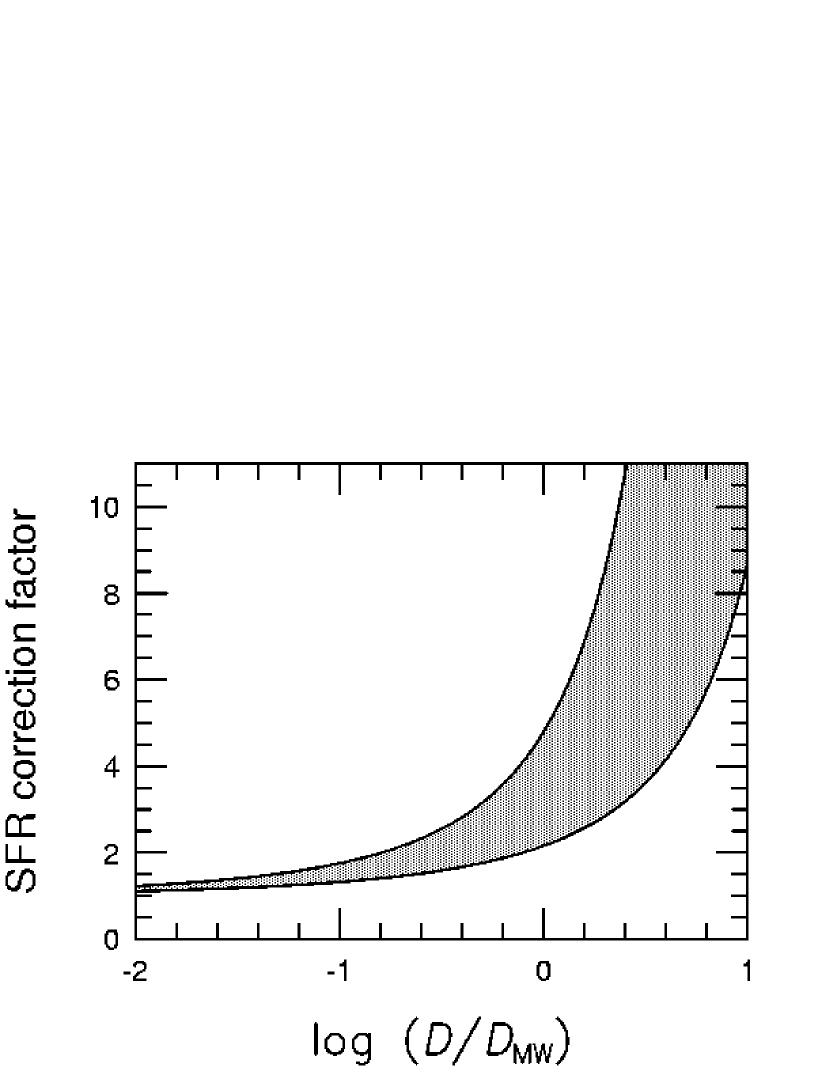
Figure 4: Correction factor for star formation rate by the LCE effect as a function of dust-to-gas ratio. The correction factor is $1/f$. The below and above lines are the case of $x=1$ and 2 in equation (5), respectively. The correction factor is expected in the shaded area between two curves.

Finally, we discuss the effect of the LCE on estimating the SFR. By the definition of $f$ in equation (1), we obtain the correction factor for the SFR by the LCE as $1/f$. If $f$ is a function of dust-to-gas ratio, the correction factor is also a function of dust-to-gas ratio. This is shown in Figure 4.

Clearly, we find that the correction factor increases as dust-to-gas ratio increases. For nearby spiral galaxies, their dust-to-gas ratios distribute around the Galactic value (Alton et al. 1998; Stickel et al. 2000, see also Paper I). Indeed, even the starburst galaxies (e.g., M82) and the ultra-luminous IR (ULIR) galaxies (e.g., Arp 220) are likely to have about the Galactic dust-to-gas ratio (Krügel, Steppe, & Chini, 1990; Lisenfeld, Isaak, & Hills, 2000). For such dust-to-gas ratio, we expect that the correction factor is 2–5. Thus, the effect of the LCE is more important than the uncertainty of the IMF, which is about a factor of 2 (e.g., Inoue et al. 2000). Therefore, we should take account of the LCE effect when we estimate the SFR of nearby spiral galaxies.

5 Conclusions

To examine the Lyman continuum extinction (LCE) in H ii regions, we compared the observed infrared emission with production rate of Lyman continuum photons for 49 H ii regions in our Galaxy, M31, M33, and LMC. Then, we estimate the fraction of Lyman continuum photons contributing to hydrogen ionization, $f$, in these regions. We reached the following conclusions:

[1] In many H ii regions, $f$ is smaller than 0.5. The mean $f$ of the sample regions in spiral galaxies (our Galaxy, M31, and M33) is about 0.4. On the other hand, the mean $f$ in the H ii regions in the LMC is about 0.7.

[2] The mean $f$ of sample H ii regions in each galaxy may be a function of metallicity or dust-to-gas ratio of their host galaxy. Namely, $f$ decreases as the metallicity or dust-to-gas ratio increases.

[3] The observational trend is reproduced very well by the model that the dust optical depth for Lyman continuum photons over the ionized region is proportional to the dust-to-gas ratio. The dust optical depth is in between 1 and 2 for the Galactic dust-to-gas ratio.

[4] It is expected that the correction factor for the star formation rate by the LCE increases as dust-to-gas ratio (metallicity) increases. The expected correction factor for the galaxies with the Galactic dust-to-gas ratio is 2–5. Therefore, the LCE effect should be taken into account when we estimate the SFR of the nearby spiral galaxies, since the dust-to-gas ratios of these galaxies are almost same as that in the Galaxy.

Table 1: The Galactic H ii regions

Object	$\log N^{\prime}_{\rm LC}$	$\log L_{\rm FIR}$	$L_{\rm IR}/N^{\prime}_{\rm LC}$	$f$
	(s-1)	($L_{\sun}$)	($10^{7}L_{\sun}/10^{50}{\rm s}^{-1}$)
(1)	(2)	(3)	(4)	(5)
NGC2024	47.7	4.3	0.40	0.40
W3	48.2	5.3	1.26	0.14
	49.4	6.1	0.50	0.32
M8	48.3	4.7	0.25	0.59
NGC6357	48.4	5.2	0.63	0.26
	48.4	5.0	0.35	0.44
IC4628	48.6	5.4	0.63	0.26
Orion	48.7	5.2	0.35	0.44
G343.4-0.4	48.7	5.5	0.56	0.29
DR15	48.8	5.8	1.12	0.15
G5.9-0.4	49.1	5.6	0.32	0.49
W75/DR21	49.2	5.3	0.13	1.01
RCW117	49.5	6.1	0.35	0.44
G351.6+0.2	49.7	6.1	0.25	0.59
W58	49.7	6.0	0.20	0.71
G351.6-1.3	49.8	6.3	0.32	0.49
W51	49.8	6.2	0.25	0.59
	50.4	6.9	0.32	0.49
RCW122	49.9	6.3	0.25	0.59
Sgr C	50.0	6.8	0.63	0.26
M17	50.1	6.5	0.25	0.59
Sgr B	50.5	7.1	0.35	0.44
W49	50.7	7.3	0.35	0.44

Note. — Col. (1): Object name. Two separate components in W3, W51, and NGC6357 are both listed. Col.(2): LC photon production rates estimated from radio observations. Col.(3): Observed FIR luminosities. Col.(4): Ratios of IR luminosity to LC photon production rates. Col.(5): Estimated $f$ from equation (2) by assuming $\epsilon=1$.

Table 2: H ii regions in M31

Object ID	$F_{60\micron}$	$L_{\rm IR}$	$F_{\rm H\alpha}$	$N^{\prime}_{\rm LC}$	$L_{\rm IR}/N^{\prime}_{\rm LC}$	$f$
	(Jy)	($10^{6}L_{\sun}$)	($10^{-12}$ erg s-1 cm-2)	($10^{50}{\rm s}^{-1}$)	($10^{7}L_{\sun}/10^{50}{\rm s}^{-1}$)
(1)	(2)	(3)	(4)	(5)	(6)	(7)
16	3.50	7.07	3.33	3.53	0.20	0.59
17	3.40	6.87	1.81	1.92	0.36	0.36
22	4.56	9.21	4.37	4.63	0.20	0.59
23	4.53	9.15	2.23	2.36	0.39	0.34
25	3.96	8.00	0.77	0.82	0.98	0.14
27	2.58	5.21	1.83	1.94	0.27	0.46
28	6.55	13.2	3.51	3.72	0.36	0.36
30	1.84	3.72	0.69	0.73	0.51	0.26
31	6.52	13.2	2.08	2.20	0.60	0.23
33	7.12	14.4	3.58	3.79	0.38	0.34
35	2.27	4.59	1.12	1.19	0.39	0.34
39	2.81	5.68	2.33	2.47	0.23	0.53

Note. — Col. (1): Identification of 60 µm sources in Xu & Helou (1996). Col.(2): Extracted 60 µm fluxes from IRAS HiRes image by Xu & Helou (1996). Col.(3): Estimated IR luminosities by adopting the distance of 760 kpc. Col.(4): H$\alpha$ fluxes corresponding with 60 µm sources. Col.(5): LC photon production rates estimated from H$\alpha$ fluxes in col.(4) by adopting the distance of 760 kpc and $A_{\rm H\alpha}=0.8$ mag. Col.(6): Ratios of IR luminosity to LC photon production rates. Col.(7): Estimated $f$ from equation (2) when we assume $\epsilon=0.7$.

Table 3: H ii regions in M33

Object	$L_{\rm FIR}$	$F_{\rm 5GHz}$	$N^{\prime}_{\rm LC}$	$L_{\rm IR}/N^{\prime}_{\rm LC}$	$f$
	($10^{7}L_{\sun}$)	(mJy)	($10^{50}{\rm s}^{-1}$)	($10^{7}L_{\sun}/10^{50}{\rm s}^{-1}$)
(1)	(2)	(3)	(4)	(5)	(6)
VGHC 20,25	0.56	0.8	0.50	1.12	0.13
IC 131	1.00	0.7	0.44	2.27	0.064
IC 133	1.67	6.6	4.14	0.40	0.33
NGC 595	0.79	18.0	11.3	0.070	1.23
VGHC 46,52	1.34	1.8	1.13	1.19	0.12
VGHC 104	0.58	1.1	0.69	0.84	0.17
VGHC 97,98	0.47	4.5	2.82	0.17	0.67
NGC 604	7.50	60.0	37.6	0.20	0.59

Note. — Col.(1): Object name. Col.(2): FIR luminosities determined from IRAS HiRes images of 60 and 100 µm by adopting the distance of 840 kpc. Col.(3): Observed 5 GHz flux densities. Col.(4): LC photon production rates estimated from col.(3) by adopting the distance of 840 kpc. Col.(5): Ratios of IR luminosity to LC photon production rates. Col.(6): Estimated $f$ from equation (2) by assuming $\epsilon=0.7$.

Table 4: H ii regions in LMC

Object	$F_{60\micron}$	$F_{100\micron}$	$L_{\rm IR}$	$F_{\rm 5GHz}$	$N^{\prime}_{\rm LC}$	$L_{\rm IR}/N^{\prime}_{\rm LC}$	$E_{B-V}$	$\epsilon$	$f$
	(Jy)	(Jy)	($10^{6}L_{\sun}$)	(Jy)	($10^{50}{\rm s}^{-1}$)	($10^{7}L_{\sun}/10^{50}{\rm s}^{-1}$)	(mag)
(1)	(2)	(3)	(4)	(5)	(6)	(7)	(8)	(9)	(10)
MC 18	1229	2029	8.48	3.37	8.03	0.11	0.07	0.28	0.68
MC 47	307	363	1.88	0.64	1.53	0.12	0.14	0.47	0.72
MC 57	337	509	2.25	0.81	1.93	0.12	0.13	0.45	0.74
MC 64	524	826	3.55	1.65	3.93	0.090	0.24	0.66	1.03
MC 71	594	819	3.83	0.55	1.31	0.29	0.11	0.39	0.34
MC 90+91	204	382	1.48	0.87	2.07	0.071	0.10	0.37	0.95

Note. — Col.(1): Object name. Cols.(2) and (3): IRAS co-added flux densities at 60 and 100 $\mu$m, respectively. Col.(4): IR luminosities determined from cols.(2) and (3). The adopted distance is 51.8 kpc. Col.(5): Observed 5 GHz flux densities. Col.(6): LC photon production rates estimated from col.(5) when the distance is adopted as 51.8 kpc. Col.(7): Ratios of IR luminosity to LC photon production rates. Col.(8): $E_{B-V}$ estimated from the observed Balmer decrement. Col.(9): $\epsilon$ determined from Figure 1. Col.(10): Estimated $f$ from equation (2).

Table 5: Summary of determined $f$ for sample galaxies

Galaxy	$f$	12+log(O/H)	$\cal D$/$\cal D_{\rm MW}$
(1)	(2)	(3)	(4)
Galaxy	$0.45\pm 0.21$	8.7	1.0
M31	$0.38\pm 0.14$	9.0	1.2
M33	$0.41\pm 0.37$	8.4	0.6
LMC	$0.74\pm 0.22$	8.37	0.2

Note. — Col.(1): Galaxy name. Col.(2): Mean $f$ with the sample standard deviation. Col.(3): Metallicity from van den Bergh (2000). Col.(4): Dust-to-gas mass ratio normalized by the Galactic value, $6\times 10^{-3}$.

Figure 1: Average extinction efficiency for nonionizing ultraviolet photons, $\epsilon$, as a function of color excess, $E_{B-V}$. The solid lines are made by using the Galactic extinction curve (Seaton, 1979). The LMC extinction curve (Howarth, 1983) results in the dashed lines. The thick lines denote the results of cases that dust albedo is set to 0.5. The thin lines are the results of no scattering.

Figure 2: Fraction of Lyman continuum photons contributing to hydrogen ionization, $f$, as a function of metallicity. The data of 12+log(O/H) are taken from van den Bergh (2000). The error bars denote the sample standard deviation of the mean presented in Table 5.

Figure 3: Fraction of Lyman continuum photons contributing to hydrogen ionization, $f$, as a function of dust-to-gas mass ratio, $\cal D$. The dust-to-gas ratio is normalized by a typical Galactic value, ${\cal D}_{\rm MW}=6\times 10^{-3}$ (Spitzer, 1978). The open square represents the case that $\cal D$ of M31 is taken from Issa et al. (1990). The error bars denotes the sample standard deviation of the mean. Two solid lines represent predictions by the model that the dust optical depth over the ionized region is proportional to $\cal D$ like equation (5).

Appendix A Infrared excess (IRE)

The IR excess (IRE) is often examined for H ii regions. We examine the relation between the LCE and IRE. Especially, we relate $f$ to IRE directly here. A concerned discussion is found in Hirashita et al. (2001).

Mezger et al. (1974) have defined the IRE as

$$IRE\equiv\frac{L_{\rm IR}}{N^{\prime}_{\rm LC}h\nu_{\rm Ly\alpha}}\,,$$ (A1)

where $h$ is the Plank constant and $\nu_{\rm Ly\alpha}$ denotes the frequency at the Lyman $\alpha$ line. From equation (A1), we obtain $L_{\rm IR,7}/N^{\prime}_{\rm LC,50}=4.23\times 10^{-2}IRE$. Therefore, equation (2) is reduced to

$$f=\frac{0.44+0.56\epsilon}{0.28+0.24IRE}\,.$$ (A2)

In Figure 5, we show the relation between $f$ and $IRE$ derived from equation (A2) for various $\epsilon$.

The solid, dotted, and dashed lines correspond to $\epsilon=1.0$ (in the Galaxy), 0.7 (in M31 and M33), and 0.4 (in LMC), respectively. In addition, we also present the dash-dotted line of $\epsilon=0$ for comparison, which corresponds to the case that no nonionizing photons are absorbed by dust. According to Spitzer (1978), the probability of producing Lyman $\alpha$ photons is two-thirds per every ionization–recombination process of hydrogen. Thus, when the observed IR luminosity of an H ii region is explained by only the luminosity of Lyman $\alpha$ photons produced in the region ($f=1$ and $\epsilon=0$), $IRE$ will be 0.67.

Antonopoulou & Pottasch (1987) have reported $4<IRE<40$ for the Galactic compact H ii regions. The mean IRE of their sample is about 12. For such high IRE regions, we expect that $f$ is about 0.3 or less. When we estimate the SFR of such regions, therefore, we should not use the H$\alpha$ or thermal radio luminosities but use the IR luminosity as an indicator of the SFR.

Figure 5: Fraction of Lyman continuum photons contributing to hydrogen ionization, $f$ as a function of infrared excess, $IRE$. The solid, dotted, dashed, and dash-dotted lines are calculated by equation (A2) with $\epsilon=$ 1.0, 0.7, 0.4, and 0, respectively.

References

- Aannestad (1989) Aannestad, P. A. 1989, ApJ, 338, 162
- Alton et al. (1998) Alton, P. B., Trewhella, M., Davies, J. I., Evans, R., Bianchi, S., Gear, W., Thronson, H., Valentijn, E., & Witt, A. 1998, A&A, 335, 807