Fast, Exact CMB Power Spectrum Estimation for a Certain Class of Observational Strategies

Abstract

We describe a class of observational strategies for probing the anisotropies in the cosmic microwave background (CMB) where the instrument scans on rings which can be combined into an n-torus, the ring torus. This class has the remarkable property that it allows exact maximum likelihood power spectrum estimation in of order $N^{2}$ operations (if the size of the data set is $N$) under circumstances which would previously have made this analysis intractable: correlated receiver noise, arbitrary asymmetric beam shapes and far side lobes, non-uniform distribution of integration time on the sky and partial sky coverage. This ease of computation gives us an important theoretical tool for understanding the impact of instrumental effects on CMB observables and hence for the design and analysis of the CMB observations of the future. There are members of this class which closely approximate the MAP and Planck satellite missions. We present a numerical example where we apply our ring torus methods to a simulated data set from a CMB mission covering a 20 degree patch on the sky to compute the maximum likelihood estimate of the power spectrum $C_{\ell}$ with unprecedented efficiency.

I Introduction

A major near-term objective in the field of Cosmology today is to gain a detailed measurement and statistical understanding of the anisotropies of the cosmic microwave background (CMB). While the theory of primary CMB anisotropy is well-developed (see [1] for a review) and we are facing a veritable flood of data from a new generation of instruments and missions, the single most limiting hurdle are the immense computational challenges one has to overcome to analyze these data[2, 3, 4].

We will now outline the key problems involved. The goal is to derive two things: an optimal sky map estimate and a set of power spectrum estimates $\widehat{C}_{\ell}$ which, for a Gaussian CMB sky are a sufficient statistic, highly informative about cosmological parameters. In this paper we will focus on the $\widehat{C}_{\ell}$ estimation problem, but the ideas we develop can be usefully employed for map-making as well [5].

We assume we start from a best estimate of the sky map of the cosmic microwave background fluctuations, the monopole and dipole components have been removed, and that residual foregrounds are negligible after excision of foreground dominated regions. The analysis problem is then one of spatial covariance estimation and involves maximizing the likelihood given the data as a function of the $\widehat{C}_{\ell}$. If the observed CMB anisotropy data is written as a vector ${\bf d}$ the likelihood takes the form

$${\cal L}(C_{\ell}|d)=\frac{\exp\left[{-\frac{1}{2}{\bf d}^{T}({\bf S}(C_{\ell})+{\bf N})^{-1}{\bf d}}\right]}{\sqrt{(2\pi)^{N_{d}}|({\bf S}(C_{\ell})+{\bf N})|}},$$ (1)

where the signal covariance matrix $\bf{S}$ is a function of the $C_{\ell}$, ${\bf N}$ is the noise covariance matrix and $N_{d}$ is the number of entries in the data vector ${\bf d}$. If ${\bf S+N}$ is a general matrix, evaluating the inverse and determinant in this quantity takes ${{\cal O}\!\left(N^{3}_{d}\right)}$ operations. For currently available data sets $N_{d}\sim 10^{5}$, which is expected to grow to $N_{d}\sim 10^{7}$ by the end of this decade.

Borrill [2] presented a careful review of the computational tasks involved in solving this maximization problem in the general case, using state-of-the-art numerical methods. The conclusion is that in their present form these methods fail to be practical for forthcoming CMB data sets. Given the major international effort currently underway to observe the CMB (see, e.g. [6, 7, 8]), finding a solution to this problem is of paramount importance.

The underlying reason for this failure is that the signal covariance matrix ${\bf S}$ and noise covariance matrix ${\bf N}$ are usually very differently structured. The data ${\bf d}$ are usually represented by a vector containing the temperatures of pixels in a sky map and $N_{d}=N_{pix}$, the number of observed pixels. Hence entries in $\bf{S}$ and ${\bf N}$ are the covariances between pairs of pixels on the celestial sphere. In pixel space, ${\bf S}$ is full, while ${\bf N}$ is ideally sparse (for a well-controlled experiment). In spherical harmonic space we are in the opposite regime. If the CMB sky is isotropic ${\bf S}$ would be diagonal for all-sky observations, while the form of ${\bf N}$ depends on experimental details and observational strategy of the mission and in general could be any covariance matrix at all. Therefore the quantity which enters in the likelihood ${\bf C\equiv S+N}$ is not sparse in any easily accessible basis. Other basis sets have been suggested, such as cut sky harmonics [9] and signal to noise eigenmodes [10, 11], but changing into these more general bases takes ${{\cal O}\!\left(N_{pix}^{3}\right)}$ operation.

There have been several attempts to find approximate formulae for the likelihood. Several methods are based on replacing the likelihood conditioned on the data vector with an approximate likelihood based on the pseudo-$C_{\ell}$ (the power spectrum computed on the incomplete sky, possibly weighted by an apodizing window)[12, 13]. These methods are very fast, scaling as ${{\cal O}\!\left(N_{pix}^{3/2}\right)}$ , unbiased, but sub-optimal to a degree which depends on the size of the survey area. A similar approach is to first compute an unbiased estimate of the correlation function in pixel space from the raw data and then transform to obtain the power spectrum in ${{\cal O}\!\left(N_{pix}^{2}\right)}$ operations[14]. A hierarchical approximation of the likelihood[15] reduces the computational scaling to ${{\cal O}\!\left(N_{pix}^{2}\right)}$ . Other authors have found minimum variance quadratic estimators[16, 17] but the calculations still require ${{\cal O}\!\left(N_{pix}^{3}\right)}$ operations.

There is only one known class of observational strategies in which the (numerically) exact maximum likelihood solution can be computed faster, namely in ${{\cal O}\!\left(N_{pix}^{2}\right)}$ operations [18]. This performance depends on a number of assumptions: azimuthally symmetric coverage of an azimuthally symmetric portion of the sky with an circularly symmetric beam and uncorrelated noise. For ease of reference we will call this class azimuthal strategies.

In this paper we discuss a second class of observational strategies, introduced in [20], for which the maximum likelihood problem can be solved exactly. This class is interesting in that it is the the first to admit fast maximum likelihood estimators which can analyze CMB data in the presence of correlated noise, non-uniform distribution of integration time, beam distortions, far side lobes, and particular types of partial sky coverage, all without needing to invoke approximations. Every forthcoming CMB datasets will be affected by some subset of these issues.

Further interest for observational strategies in this class derives from the fact that they are natural choices from a practical point of view. Evidence for this is that current and future balloon and space missions have chosen strategies which are based on scanning on interlocked rings: Archeops scanned on rings, MAP’s precessing scan generates a 3-torus, and the simplest of the proposed scanning strategies for Planck generates a 2-torus.

The key point is that for this class of observational strategies modeling observations in the time ordered domain simplifies the problem greatly. In section II we argue that several instrumental effects are modelled more easily in the time ordered data (TOD). To be able to formulate the likelihood problem in terms of the TOD one needs to be able to compute the expected signal covariance between two samples in the TOD. We achieve this using the Wandelt-Górski method for fast convolution on the sphere [22] which we briefly review in section III.

Using the results from these geometrical ideas we go on to formulate the likelihood problem for the $C_{\ell}$ on the ring torus in section IV. We show that the correlation matrices have a special structure for a class of scanning strategies namely those where the TOD can be thought of as being wrapped on an n-torus, the ring torus. It turns out that both ${\bf S}$ and ${\bf N}$ are sparse. In fact, they are both block-diagonal with identical patterns of blocks; hence ${\bf C}$ is also block diagonal. The exact computational scaling of the evaluation of ${\cal L}(C_{\ell})$ depends on the scanning strategy used, but if the ring torus is an 2-torus it takes only ${{\cal O}\!\left(N_{d}^{2}\right)}$ operations.

We then present a numerical example where er apply this method to simulated data in section V. Finally, we discuss the application of our ideas to real world missions and conclude with suggestions for future directions in section VI.

II The Case for Analyzing CMB Data in the Time-Ordered Domain

In this section we will discuss features of realistic instruments and observational strategies and show that they are more easily modeled in the time ordered domain.

A Correlated noise

Current detectors have the feature that they add correlated noise to the signal. It appears to be a good approximation to assume that this noise is stationary and circulant. If this is the case then it has a very simple correlation structure in Fourier space. But estimating the sky from the TOD projects these simple correlations into very complicated noise correlations between separated pixels, which are visible as striping in the maps.

B Non-uniform distribution of integration time

For most missions, practical constraints on the scanning strategy force the available integration time to be allotted non-uniformly over the sky. This leads to coupling of the noise in spherical harmonic space, in addition to coupling due to partial sky coverage (see paragraph D below). However, in the TOD, integration time per sample is constant, by definition.

C Beam distortions and far side lobes

Microwaves are macroscopic, with wavelengths of order $10^{-3}$ — $10^{-2}$cm. Hence they will diffract around macroscopic objects. This leads to distorted point spread functions and far side lobes. Simulations have to convolve these asymmetric beams with an input sky with foreground signals varying over many orders of magnitude from place to place. Motions of the instrument while a sample is taken leads to anisotropic smearing of the beam. Analyses have to deconvolve the observations to make accurate inferences about the underlying sky. Artifacts due to asymmetric beams and beam smearing affect the correlations of the signal in a raw, coadded sky map in a complicated way which depends on the scanning strategy of the instrument. If the beam is short in a particular direction, the data contains information on this short scale. Deconvolution can in principle reveal additional structure.

D Partial sky coverage

The cosmological information is most visible in spherical harmonic space. In a homogeneous and isotropic Universe, where the perturbations are Gaussian, the power spectrum $C_{\ell}$ completely encodes the statistical information which is present in a map of fluctuations. Statistical isotropy of the fluctuations around us also implies that the spherical harmonics $Y_{\ell m}$ are the natural basis for representing the CMB sky. But due to astrophysical foregrounds that need to be excised from the map or partial sky coverage by the instrument this isotropy is broken in actual data sets. This introduces additional signal and noise correlations in $Y_{\ell m}$ space, because there is a geometrical coupling between $Y_{\ell m}$ of different $\ell$ and $m$.

E Pixelization effects

Representing the data as a pixelised map on the sky is an invaluable and time-proven tool for visual analysis. However, it is not without possible disadvantages either. Binning samples into discrete sky pixels introduces an extra level of smoothing on the pixel scale and erases information, for example the exact distribution of sampling locations. Too large pixels will degrade the signal and erase information about the beam shape (cf issue C). If the distribution of samples on the sky is non-uniform choosing pixels too small will result in many missing pixels and hence irregularly shaped observation regions.

There are currently no exact and fast methods that can deal with all of these issues. Yet, every forthcoming CMB dataset will be affected by some subset of these issues.

It is clear from A and B that the noise properties are much simpler in the TOD than in a sky map. But what about the signal correlations? What is the price of forfeiting the advantages of the sphere for representing statistically isotropic signals? In the next section we will demonstrate that one can devise scanning strategies which break only part of the symmetries of the sphere and make the signal correlations in the TOD as simple as the noise properties.

III Modeling the Signal in the Time-Ordered Domain

Recently, Wandelt and Górski [22] have introduced new methods for greatly speeding up convolutions of arbitrary functions on the sphere. This reference contains a detailed description of methods which will enable future missions such as MAP and Planck to take beam imperfections into account without resorting to approximations. The algorithm is completely general and can be applied to any kind of directional data, even tensor fields [23]. We will now briefly review the ideas and quote the results.

Let us define more precisely what is meant by “convolution on the sphere”. Mathematically, the convolution of two functions on the sphere is a function over the group of rotations SO(3), because one has to keep track of the full relative orientation of the beam to the sky, not just the direction it points in. For each possible relative orientation (element of SO(3)) the convolution returns one value. To specify the relative orientation one can use the Euler angles $\Phi_{1},\Theta$ and $\Phi_{2}$. The convolved signal for each beam orientation $(\Phi_{1},\Theta,\Phi_{2})$ can then be written as

$$T^{S}(\Phi_{2},\Theta,\Phi_{1})=\int d\Omega_{\vec{\gamma}}\,\left[\widehat{D}(\Phi_{2},\Theta,\Phi_{1})b\right]\!\!(\vec{\gamma})^{\ast}s(\vec{\gamma}).$$ (2)

Here the integration is over all solid angles, $\widehat{D}$ is the operator of finite rotations such that $\widehat{D}b$ is the rotated beam, and the asterisk denotes complex conjugation. At each point on the sphere, there is a ring of different convolution results corresponding to all relative orientations about this direction. This is a direct consequence of the fact that the beam is not assumed to be azimuthally symmetric.

If ${\sf{L}}$ measures the larger of the inverse of the smallest length scale of the sky or beam, the numerical evaluation of the integral in Eq. (2) takes ${{\cal O}\!\left({\sf{L}}^{2}\right)}$ operations for each tuple $(\Phi_{1},\Theta,\Phi_{2})$. To allow subsequent interpolation at arbitrary locations it is sufficient to discretize each Euler angle into ${{\cal O}\!\left({\sf{L}}\right)}$ points and thus we have ${{\cal O}\!\left({\sf{L}}^{3}\right)}$ combinations of them. As a result, the total computational cost for evaluating the convolution using Eq. (2) scales as ${{\cal O}\!\left({\sf{L}}^{{5}}\right)}$ .

It turns out that by Fourier transforming the above equation on the Euler angles and judiciously factorising the rotation operator $\widehat{D}(\Phi_{2},\Theta,\Phi_{1})$ as described in [22] we can reduce this scaling to ${{\cal O}\!\left({\sf{L}}^{{4}}\right)}$ in general. One can further reduce the scaling to ${{\cal O}\!\left({\sf{L}}^{3}\right)}$ if one is only interested in the convolution over a path which consists of a ring of rings at equal latitude around the sphere. We called such configurations basic scan paths in references [22, 20].

We quote here the formula for the Fourier coefficients of the convolved signal on this ring torus using the notation of [22]. In order to do so we need to make use of the angular momentum representation of the rotation operator $\widehat{D}$. A simple explicit expression for the matrix elements $D^{l}_{mm^{\prime}}(\phi_{2},\theta,\phi_{1})$ can be given. One can define a real function $d^{l}_{mm^{\prime}}(\theta)$ such that

$$D^{l}_{mm^{\prime}}(\phi_{2},\theta,\phi_{1})=e^{-im\phi_{2}}d^{l}_{mm^{\prime}}(\theta)e^{-im^{\prime}\phi_{1}}$$ (3)

Thus the dependence of $D$ on the Euler angles $\phi_{1}$ and $\phi_{2}$ is only in terms of complex exponentials. While explicit formulas for the $d$-functions exist [24], they are more conveniently computed numerically using their recursion properties [25].

If the convolved signal on the ring torus is $T^{S}_{rp}$ with $r$ counting the ring number and $p$ the pixel number on the ring, then its Fourier coefficients are

$$\widetilde{T}^{S}_{m\,m^{\prime}}=\sum_{\ell}s_{\ell m}d^{\ell}_{mm^{\prime}}(\theta_{E})X_{\ell m^{\prime}}.$$ (4)

Here the $s_{\ell m}$ are the spherical harmonic multipoles for the CMB sky and $\theta_{E}$ fixes the latitude of the spin axis on the sky. The quantity

$$X_{\ell m}\equiv\sum_{M}d^{\ell}_{mM}(\theta)b_{\ell M}^{\ast}$$ (5)

is just the rotation of the beam multipoles $b_{\ell m}$ for an arbitrary beam by $\theta$, the opening angle of the scan circle. $X_{\ell m}$ can be precomputed. Counting indices in Eq. (4) confirms that computing the convolution along a basic scan path takes only ${{\cal O}\!\left({\sf{L}}^{3}\right)}$ operations.

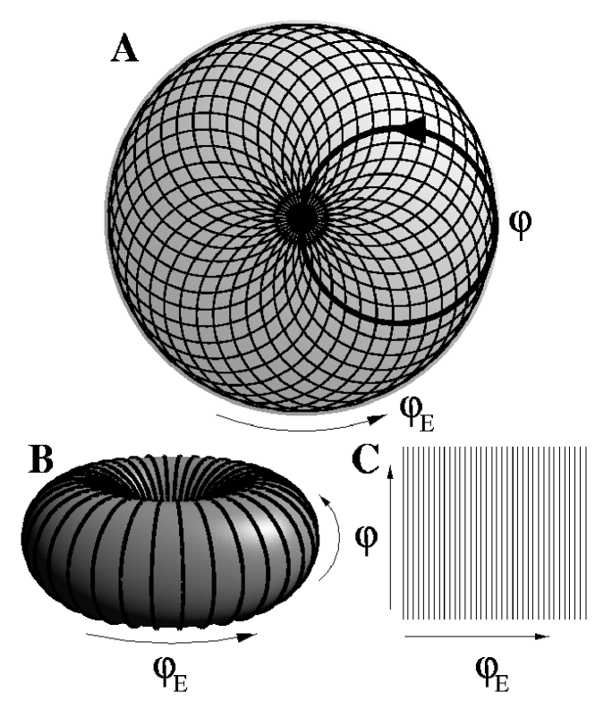
FIG. 1.: The ring torus in three different representations. Figure A shows the scan rings on the sphere for one particular scanning strategy. We see the projection of a disc $20^{\circ}$ across, covered with rings of radius $\theta=5^{\circ}$ whose centers are $\theta_{E}=5^{\circ}$ away from the north pole. The angles $\phi$ and $\phi_{E}$ parametrize the position on each ring and the ring location, respectively. Figure B shows the 2 dimensional ring torus generated by this scanning strategy and in Figure C the rings are unfolded into a 2 dimensional plane like in Figures (3) and (4).

IV Likelihood Analysis on the Ring Torus

Using the results from the previous section we can now write down a statistical model in terms of the likelihood of the $C_{\ell}$ and experimental parameters given the time-ordered data.

We will first derive the signal-correlation matrix as a function of the $C_{\ell}$ and then go on to derive the noise correlation as a function of instrumental parameters (like the shape of the noise power spectrum in the TOD) and the scanning strategy (in this case the dimensions and position of the basic scan path).

A Signal Correlations

What we are interested in are the correlation properties of the signal on the ring torus, Eq. (4). We can now easily compute the correlation matrix

$${\cal T}^{S}_{m\,m^{\prime}\;M\,M^{\prime}} \equiv \left\langle T^{S}_{m\,m^{\prime}}T^{S}_{M\,M^{\prime}}\right\rangle$$ (6)

$$= \framebox{$\delta_{mM}$}\sum_{\ell}C_{\ell}d^{\ell}_{mm^{\prime}}(\theta_{E})X_{\ell m^{\prime}}d^{\ell}_{MM^{\prime}}(\theta_{E})X_{\ell M^{\prime}}.$$ (7)

where $\delta_{ij}$ denotes the Kronecker delta, defined as

$$\delta_{ij}=\left\{\begin{array}[]{ll}1&{\rm if}~{}i=j\\ 0&{\rm if}~{}i\neq j\\ \end{array}\right..$$ (8)

The boxed Kronecker delta shows that the correlation matrix in Fourier space on the ring torus is block diagonal.

B Noise Correlations

We start by assuming that we can model the noise in the time ordered domain as a stationary Gaussian process whose Fourier components $\widetilde{T}^{N}_{k}$ have the property

$$\left\langle\widetilde{T}^{N}_{k}\widetilde{T}^{N\ast}_{k^{\prime}}\right\rangle=P(k)\delta_{kk^{\prime}}.$$ (9)

In the following we will allow for the complication that the scanning strategy involves integrating repeatedly on a fixed ring then the signal remains the same for each scan of that ring. One can just co-add all scans over the same ring without losing information.

To be specific, if we define $N_{R}$ to be the number of pixels per ring, $N_{c}$ the number of times the satellite spins while observing a fixed ring, and $N_{r}$ to be the number of rings for a one-year mission, we can write $N_{TOD}=N_{R}N_{c}N_{r}$ for the number of samples in the TOD. In the following we will choose $N_{r}=N_{R}$ for simplicity, though this is not required by the formalism and can be generalised trivially.

To model the noise on the coadded rings, we define $T_{pr}$ to be the noise temperature in the $p$th pixel in the $r$th ring, such that

$$T_{pr}\equiv\sum_{n=0}^{N-1}A_{pr\,n}T_{n}.$$ (10)

Here $A_{pr\,n}$ is the co-adding matrix, defined in Eq. (A1). It encodes the scanning strategy by associating a given pixel in the ring set with indices $r$ and $p$ with a set of samples in the TOD.

Then we can show (see Appendix) that the covariance matrix of the Fourier components of the co-added noise on the rings is

$${\cal T}^{N}_{m^{\prime}mM^{\prime}M} \equiv \left\langle\widetilde{T}^{N}_{m^{\prime}m}\widetilde{T}^{N\ast}_{M^{\prime}M}\right\rangle$$ (11)

$$= \frac{1}{(N_{r})^{3}}\framebox{$\delta_{mM}$}\sum_{p,p^{\prime}=0}^{N_{r}-1}e^{-\frac{2\pi i}{N_{r}}(m^{\prime}p-M^{\prime}p^{\prime})}\sum_{\Delta=0}^{N_{r}-1}e^{-\frac{2\pi i}{N_{r}}m\Delta}C(\Delta,p-p^{\prime})$$ (12)

where $C(\Delta,p-p^{\prime})$ is defined in Eq. (A2). The boxed Kronecker-$\delta$ is telling us that the noise covariance is block diagonal in the ring Fourier basis.

C Generalization to more complicated scanning strategies

We just showed that by choosing the scanning strategy such that the TOD can be wrapped (co-added) onto a 2-torus one can find a basis in which both noise and signal are block diagonal and hence sparse. What is more, the data can be easily transformed into this basis just by computing the Fast Fourier Transform (FFT) of the co-added TOD.

The results Eq. (7) and Eq. (11) warrant some comments. We can understand them in terms of symmetries. The ring torus exhibits a spatio-temporal symmetry: time proceeds linearly around the torus, in the same direction as the azimuthal angle $\phi_{E}$ (cf. Fig. (1)). Wrapping the TOD on the torus breaks the translation invariance of the noise in the TOD. Similarly, projecting the signal from the sphere onto the torus breaks the isotropy of the signal on the sphere. But these original symmetries manifest themselves as ring–stationarity of the noise (correlations between rings only depend on the distance between them) and ring–stationarity/“partial isotropy” of the signal (only in the azimuthal $\phi_{E}$ direction on the torus). These in turn express themselves as a simplified correlation structure in Fourier space.

We can therefore see that the key feature which leads to the simplicity of the correlation matrices is the repetitive structure of the scanning in the $\phi_{E}$ direction. Therefore it is plain that these methods can be generalised to ring tori of arbitrary cross section, for example where the scanning rings are ellipses, without losing the computational scaling performance, albeit with more cumbersome formulae which we will not produce here in detail. This would also enable us to remove regions where foregrounds dominate if that involved removing the same part of every ring in the torus, because this does not spoil the ring–stationarity.

From following the discussion in [22] we can easily see how the results Eq. (7) and Eq. (11) generalize to precessing scans. For example rewriting Eq. (8) in [22] as

$$T_{m\,m^{\prime}\,m^{\prime\prime}}=\sum_{\ell}s_{\ell m}d^{\ell}_{m\,m^{\prime}}(\theta_{E})d^{\ell}_{m^{\prime}m^{\prime\prime}}(\theta_{P})X^{\;\ast}_{\ell m^{\prime\prime}}.$$ (13)

and substituting for $X_{\ell m^{\prime\prime}}$ from Eq. (5) we obtain the signal part of the TOD for a precessing experiment where the spin axis moves around the sphere at co-latitude $\theta_{E}$ and precesses about it with amplitude $\theta_{P}$. We see that this TOD can be wrapped on a 3-torus. Computing the signal correlation matrix in Fourier space on this 3-torus ${\cal T}^{S}_{m\,m^{\prime}\,m^{\prime\prime}\;M\,M^{\prime},M^{\prime\prime}}$ we find that it is again block diagonal. However, the size of blocks has now increased. The computational performance in this case depends on the details of the scanning strategy, but in general will lead to a prefactor which increases with the precession angle $\theta_{P}$.

For completeness we mention that by introducing further factors of the rotation operator this formalism can be generalised to n-tori with $n>3$, but this would appear to give rise to impractical scanning strategies.

D Constructing the likelihood for ring torus power spectrum estimation

One can write down the likelihood Eq. (1) on the ring torus by simply substituting

$$d_{\rm map}\rightarrow d_{\rm ring~{}torus},\quad{\bf S}\rightarrow{\cal T}^{S},\quad{\bf N}\rightarrow{\cal T}^{N}.$$ (14)

Due to the block diagonality, the inverse and determinant in the Eq. (1) only take ${{\cal O}\!\left(N^{2}\right)}$ operations to evaluate. The gradient is similarly easy to evaluate

$$-2\frac{\partial\ln{\cal L}}{\partial C_{\ell}}=Tr({\bf C}^{-1}{\bf C,}_{C_{\ell}})-d^{T}{\bf C}^{-1}{\bf C,}_{C_{\ell}}{\bf C}^{-1}d$$ (15)

which only takes ${{\cal O}\!\left({\sf{L}}^{3}\sim N^{3/2}\right)}$ operations to compute for each component.

E Confidence Regions

To determine confidence regions for the estimates one could explore the likelihood surface around the maximum. If the number of estimated band powers is $N_{b}$, using this recipe to evaluate the diagonal elements of the covariance matrix of the estimates would scale as ${{\cal O}\!\left(N_{b}N^{2}\right)}$ , and the full covariance ${{\cal O}\!\left(N_{b}^{2}N^{2}\right)}$ . This is more like ${{\cal O}\!\left(N^{5/2}\right)}$ or ${{\cal O}\!\left(N^{3}\right)}$ depending on the coarseness of the binning.

But one can improve on this, because evaluating the gradient of the likelihood also takes just ${{\cal O}\!\left(N^{2}\right)}$ operations on the ring torus. So one can numerically differentiate the gradient with respect to the $i$-th band power estimate, to obtain the i-th row of the covariance matrix. The full covariance matrix can then be computed in ${{\cal O}\!\left(N_{b}N^{2}\right)}$ operations. That’s at most ${{\cal O}\!\left(N^{5/2}\right)}$ but given that the $C_{\ell}$ are smooth in most models $N_{b}\lesssim 100$ may suffice, especially for less than full sky coverage, where adjacent $C_{\ell}$ estimates become strongly coupled.

V Numerical Example: Power Spectrum Estimation

To test the method, we used a standard CDM power spectrum and simulated a realization of spherical harmonic multipoles $a_{\ell m}$ up to ${\sf{L}}=1024$. We used the Wandelt-Górski method for fast convolution to generate $N_{r}=243$ scanning rings with $5^{\circ}$ radius $N_{R}=243$ samples each. The spin axis was offset from the north pole by $5^{\circ}$. This scanning pattern is shown in Fig. (1A). The data covers a polar cap on the sphere of diameter 20 degrees. For simplicity we used a symmetric Gaussian beam with full width at half maximum of $18^{\prime}$ – however this simplification is not forced by the method which allows using any beam pattern.

FIG. 2.: The noise model in the time ordered data. The vertical line shows the knee frequency. The frequency $k$ is shown in units of the Nyquist frequency of the time stream $N_{TOD}/2$.

For the noise power spectrum we use a simple model motivated by measurements from realistic receivers – but again any power spectrum could be used here. We adopot the functional form used by [26, 27]

$$P(k)=2\sigma^{2}[1+(k_{knee}/k)^{\alpha}],\qquad 0<\alpha\leq 2,$$ (16)

where the first term corresponds to white noise with variance per pixel of $\sigma^{2}$ and the second to $1/f$–type noise. We show this power spectrum in Fig. (2). For our simulations we regularize this form at small frequency by introducing a small additive constant corresponding to a tenth of the smallest representable frequency in the denominator of the $1/f$ term. Hence our noise simulation is not constrained to have zero mean but contains a random offset.

We generated a realisation of noise with $\alpha=1$, $\sigma=9\mu K$ and $k_{knee}=1.\times 10^{-3}$ (expressed in terms of the Nyquist frequency $N_{TOD}/2$) and added it to the ring set. The value of $\sigma$ was chosen to give $S/N\sim 1$ at $\ell=600$ for our simulations. We have $N_{r}=243$ rings with $N_{R}=243$ pixels in each ring. For simplicity of implementation each ring was scanned a single time, $N_{c}=1$, giving a total number of $N_{TOD}=59049$ pixels, a similar number of pixels to the BOOMERAnG experiment.

In Fig. (3) we show the ringset with and in Fig. (4) without noise using the representation shown in Fig. (1C). On the plots, a line from the top to the bottom describes one ring, in this way the rings are put next to each other from left ro right. The line from left to right in the middle, with the same value, is the north pole where all rings meet. We see clearly the stripes from the correlated noise.

Instead of estimating $C_{\ell}$, we estimate $D_{\ell}$ given by,

$$D_{\ell}=\frac{C_{\ell}\ell(\ell+1)}{e^{-\sigma_{b}^{2}\ell(\ell+1)}},$$ (17)

where $\sigma_{b}$ is for a $18^{\prime}$ FWHM beam. We divide $D_{\ell}$ in $N_{b}=20$ flat bins $D^{1},D^{2},...,D^{20}$ with $50$ multipoles in each.

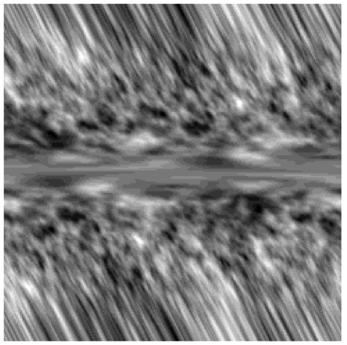
FIG. 3.: The ring set from a scan on a simulated sky without noise. On the plot, a line from the top to the bottom describes one ring. In this way the rings are put next to each other from left ro right. The north pole gets mapped in to the horizontal line of constant value in the middle of the plot. All rings touch there.

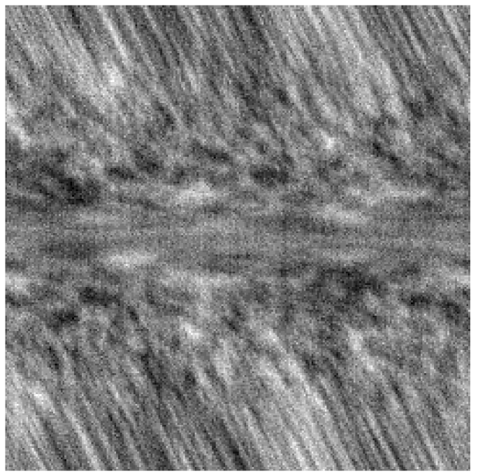
FIG. 4.: As Fig. (3) but with correlated noise added, causing the vertical striping.

The Fourier transformed signal correlation matrix can be calculated in two ways. One might evaluate it directly in Fourier space with equation (7), or one could first evaluate it in pixel space and then Fourier transform it using FFT. In our test example we have chosen the latter. The formula for the correlation matrix in pixel space is in our case

$$<T_{pr}T_{p^{\prime}r^{\prime}}>=\sum_{b}D^{b}\sum_{\ell\epsilon b}\frac{e^{-\sigma_{b}^{2}\ell(\ell+1)}}{\ell(\ell+1)}\frac{2\ell+1}{4\pi}P_{\ell}(\cos\delta\theta),$$ (18)

where $\delta\theta$ is the angular distance between the two points $pr$ and $p^{\prime}r^{\prime}$ on the sphere and the sum over $\ell$ is taken over all $\ell$ values in the particular bin $b$. All $\delta\theta$ angles are precomputed. The derivative with respect to a certain bin is then simply,

$$\frac{\partial<T_{pr}T_{p^{\prime}r^{\prime}}>}{\partial D^{b}}=\sum_{\ell\epsilon b}\frac{e^{-\sigma_{b}^{2}\ell(\ell+1)}}{\ell(\ell+1)}\frac{2\ell+1}{4\pi}P_{\ell}(\cos\delta\theta),$$ (19)

In Figure (5) we have plotted the result from likelihood estimation. To find this estimate we initialised the iterative conjugate gradient scheme [28] with a flat power spectrum $C_{\ell}=$constant. The minimum of the likelihood was found after about 30 function and derivative evaluation taking about 2 hours each on a single processor on a 500 MHz DEC Alpha Work Station. If we had started the likelihood minimisation with a better inital guess for the power spectrum (which could be obtained using one of the $N^{3/2}$ methods [12, 13]) the number of likelihood evaluations could be significantly reduced.

FIG. 5.: The result from a likelihood estimation of the power spectrum from a time stream with 243 rings with 243 pixel per ring. The error bars approximate asymmetric $2\sigma$ confidence regions by showing where the loglikelihood drops by less than $2$ compared to the maximum. Three points at high $\ell$ fail to detect significant power at 95% confidence and return upper limits on $C_{\ell}$.

The solid line shows the input average power spectrum used and the crosses are the estimates with error bars. The errorbars approximate a 95% confidence region determined by finding the interval of the estimate where the log-likelihood is reduced by less than 2 compared to its maximum value. We compared these confidence regions with the errors bars determined from the observed Fisher matrix by finding the numerical second derivative of the loglikelihood. The square root of the diagonal components of its inverse yields errorbars which were consistent with the ones we obtained from the likelihood contours.

Note that we did not subtract lower order modes from the sky patch that we simulated (though we assumed that the map was free of non-cosmological monopole and dipole modes). As we mentioned, the noise was also not constrained to average to zero. The presence of lower order modes was correctly modelled and handled by the algorithm.

VI Critical Discussion and Conclusions

In this paper we described the properties of the class of observational stratgies where the instrument scans on rings which can be arranged into an n-torus. Using these properties we constructed for the first time an exact formulation of the maximum likelihood problem of power spectrum analysis on the sphere which can deal with correlated noise, realistic beams, partial sky coverage, and non-uniform noise with a computational scaling of ${{\cal O}\!\left(N^{2}\right)}$ . This is a significant advance over other available exact methods with the same scaling, all of which assume white noise and azimuthally symmetric beams, amongst other assumptions.

How realistically can we expect these methods to be useful for real CMB missions? Real observations obviously never coincide exactly with any simple mathematical model. This was also true for the previously known solvable class of strategies of azimuthal sky coverage, symmetric beams and uncorrelated noise. But the fact that the likelihood simplifies in this idealised situation, defined one of the design goals for the MAP satellite, namely to ensure that the noise be uncorrelated between samples. This allowed a fast maximum likelihood power spectrum estimation method to be developed for MAP [18] which achieves success by employing iterative numerical schemes taking advantage of the fact that the data nearly satisfy the assumptions of the exactly solvable case and thus improve convergence. Perturbation theory is powerful but only if exact solutions are known that are close to the real thing.

In our case, even though the methods we describe can deal with many features of actual CMB missions, there remain discrepancies. We have not shown (except for our discussion in section IV C) how to deal with small areas where foregrounds dominate and defy removal, such as bright dust emission from the galactic plane, or certain point sources. Also, irregularities in the scanning strategy will somewhat spoil the symmetry of spatial correlations in the signal and temporal correlations in the noise which the ring torus exploits.

We therefore advocate a similar approach to the one which was used successfully in [18], namely to use exact inverses, computed using the methods we presented in this paper as preconditioners to speed up conjugate gradient methods for computing $C^{-1}d$ for more general cases, e.g. galactic cuts, point sources, imperfect scanning and non-stationarity of the noise. Other nuisance factors, such as discrete events like cosmic ray hits and short telemetry losses can plausibly be dealt with in established ways, namely by filling in the data stream with a constrained realisation based on the properties of the observed data.

Even neglecting the computational advantages of ring torus methods there are other advantages to analysing time ordered data directly. First, this approach does not rely on map-making on the sphere for the purposes of power spectrum estimation. Not having to base $C_{\ell}$ estimation on maps helps to avoid systematic effects or signal degradation introduced by previous analysis steps, for example a heuristic de-striping tool. On the ring torus, one fully models the striping due to correlated noise and hence does not rely on heuristic methods.

While the sky map may not necessarily be the best starting point for the purposes of $C_{\ell}$ estimation, one should of course make the best map one possibly can. Maps are indispensable for the visualization of the data and identifying systematic errors. Also, recently developed map based methods for estimating the noise properties of the observations from the data itself [29, 30] can be used to provide the necessary noise model input to our methods (such as $P(k)$, Eq. (16)).

In fact the geometrical ideas we discuss in this paper may well be useful for map making itself. Reference [22] shows how the ring torus speeds up iterative methods for deconvolving a map with asymmetric beams. The block diagonal noise correlations on the torus mean that one can use the same geometrical ideas for solving the map making equations in the presence of noise. In fact both signal and noise covariances are sparse in this basis, hence this method can be used to quickly Wiener filter the data on the ring torus once the $C_{\ell}$ are known to optimally estimate the CMB fluctuations on the torus. These can then be visualized by projecting them onto a sky map.

Under the stated assumptions we have shown that the power spectrum analysis problem simplifies greatly when it is considered in the domain of co-added time-ordered data which has the geometry of a torus. We indicate how to derive extensions of the formulae we presented here to more general scanning strategies (e.g. a precessing scan, such as MAP’s or another proposal for Planck). In this case the efficiency depends on the size of the extra dimensions which the torus acquires.

However, even as they stand, the methods and ideas we describe represent a new theoretical tool which allows evaluating the impact of CMB mission design choices in much more detail than previously feasible. In order to achieve the best possible estimates of the CMB power spectrum, or certain cosmological parameters, one can ask whether it is more important to reduce the amount of correlated noise from the receiver, to ensure accurate pointing, to increase sky coverage, change the survey geometry, or to control the beam shape and far side lobes? We are investigating quantitative answers to these questions.

A The Noise Covariance on the ring torus

The co-adding matrix can be written as

$$A_{pr\,n}\equiv\frac{1}{N_{c}}\delta_{p(n\mod N_{r})}\delta_{r\left(\left\lfloor\frac{n}{N_{r}N_{c}}\right\rfloor\right)}=\frac{1}{N_{c}}\delta_{rx}\delta_{pz}$$ (A1)

Here $\lfloor f\rfloor$ is defined to be the largest integer smaller than $f$.

The previous equations simplify if we write $n$ as $n=N_{r}N_{c}x+N_{r}y+z$ with $x\in[0,N_{r}-1]$, $y\in[0,N_{c}-1]$, $z\in[0,N_{r}-1]$. Now using that

$\displaystyle<T^{N}_{n}T^{N}_{n^{\prime}}>=\sum_{k}e^{\frac{-2\pi ik}{N}(n-n^{\prime})}P(k),$

we find that the noise covariance on the ring set is

$$C(r-r^{\prime},p-p^{\prime})\equiv\left\langle{T}^{N}_{rp}{T}^{N\ast}_{r^{\prime}p^{\prime}}\right\rangle=\frac{1}{N_{c}^{2}}\sum_{k=0}^{N-1}P(k)\sum_{y,y^{\prime}=0}^{N_{c}-1}e^{{-\frac{2\pi ik}{N}(N_{r}N_{c}(r-r^{\prime})+N_{r}(y-y^{\prime})+(p-p^{\prime}))}}.$$ (A2)

Note that $C$ is periodic with period $N_{r}$ in its first entry; letting $\Delta\equiv r-r^{\prime}$ we have

$$C(\Delta,p-p^{\prime})=C(\Delta+jN_{r},p-p^{\prime}),\quad j\in{\cal Z}.$$ (A3)

Finally we Fourier transform to arrive at the covariance of the Fourier components of the the co-added noise on the rings

$${\cal T}^{N}_{m^{\prime}mM^{\prime}M} \equiv \left\langle\widetilde{T}^{N}_{m^{\prime}m}\widetilde{T}^{N\ast}_{M^{\prime}M}\right\rangle$$ (A4)

$$= \frac{1}{(N_{r})^{3}}\framebox{$\delta_{mM}$}\sum_{p,p^{\prime}=0}^{N_{r}-1}e^{-\frac{2\pi i}{N_{r}}(m^{\prime}p-M^{\prime}p^{\prime})}\sum_{\Delta=0}^{N_{r}-1}e^{-\frac{2\pi i}{N_{r}}m\Delta}C(\Delta,p-p^{\prime})$$ (A5)

where we used (A3) to simplify the sums over $r,r^{\prime}$ and to obtain the boxed Kronecker-$\delta$ telling us that the noise covariance is block diagonal in the ring Fourier basis.

For practical purposes one would first compute the Fourier transfrom in (A2) using an FFT taking $\sim N\log N$ operations. Then the resulting array can be interpolated at $N_{r}(2N_{r}-1)$ positions to obtain the independent components of $C$. Finally we have a three-dimensional FFT left to evaluate (11), which requires $N_{r}^{3}\log N_{r}$ operations.

REFERENCES

- [1] W. Hu, N. Sugiyama, and J. Silk, Nature 386, 37 (1997).
- [2] J. Borrill, Phys. Rev. D59, 027302 (1999).
- [3] K. M. Gorski, E. F. Hivon and B. D. Wandelt,Analysis Issues for Large CMB Data Sets, astro-ph/9812350, in “Evolution of Large Scale Structure”, A. J. Banday et al. (Eds) (1998).
- [4] J. R. Bond, R. G. Crittenden, A. H. Jaffe, and L. Knox, Computing in Science and Engineering 1, (1999).
- [5] A. Challinor et al., in preparation.
- [6] Tophat WWW-site, http://topweb.gsfc.nasa.gov/
- [7] Bennett, C. L. et al. 1996, Microwave Anisotropy Probe: A MIDEX Mission Proposal, see also http://map.gsfc.nasa.gov/
- [8] Bersanelli et al. 1996, COBRAS/SAMBA: Report on the Phase A Study, see also http://astro.estex.esa.nl/Planck/.
- [9] K. M. Gorski, Astrophys. J. Lett., 430, L85 (1994).
- [10] J. R. Bond, Phys. Rev. Lett. 74, 4369 (1995)
- [11] M. Tegmark, A. Taylor, and A. Heavens, Astrophys. J. 480, 22 (1997).
- [12] B. D. Wandelt, E. F. Hivon, K. M. Gorski, astro-ph/9808292; B. D. Wandelt, K. M. Gorski, E. F. Hivon, astro-ph/0008111, Phys. Rev. D in press.
- [13] E. Hivon et al., MASTER of the CMB Anisotropy Power Spectrum: A Fast Method for Statistical Analysis of Large and Complex CMB Datasets, astro-ph/0105302
- [14] I. Szapudi et al., Fast CMB Analyses via Correlation Functions, astro-ph/0010256
- [15] O. Dore, L. Knox, A. Peel,CMB Power Spectrum Estimation via Hierarchical Decomposition, astro-ph/0104443
- [16] M. Tegmark, Phys. Rev. D 55, 5895 (1997)
- [17] J. R. Bond, A. H. Jaffe, and L. Knox, Phys. Rev. D57, 2117 (1998)
- [18] S. P. Oh, D. N. Spergel, and G. Hinshaw, Astrophys. J. 510, 551 (1999).
- [19] The HEALPIX homepage: http://www.eso.org/kgorski/healpix/
- [20] B. D. Wandelt,Advanced methods for cosmic microwave background data analysis: the big and how to beat it, astro-ph/0012416, in proceedings of MPA/ESO/MPE Joint Conference ”Mining the Sky”, Garching bei Muenchen, A.J. Banday et al. (Eds). (2000)
- [21] J. Delabrouille, K. M. Górski, and E. Hivon, MNRAS 298, 445 (1998)
- [22] B. D. Wandelt and K. M. Górski, Phys. Rev. D63, 123002 (2001)
- [23] A. Challinor et al., Phys. Rev. D62, 123002 (2000)
- [24] D. A. Varshalovich, A. N. Moskalev, and V. K. Khersonskii, Quantum Theory of Angular Momentum (Singapore: World Scientific, 1988); D. M. Brink and G. R. Satchler, Angular Momentum (Clarendon Press, Oxford, 1975).
- [25] T. Risbo, Journal of Geodesy 70, 383 (1996).
- [26] D.Maino et al., A&AS 140, 383 (1999)
- [27] J. Delabrouille, A&AS 127, 555 (1998)
- [28] W. H. Press et al., Numerical Recipes in Fortran: The Art of Scientific Computing, 2nd Edition (Cambridge University Press, 1992)
- [29] P. G. Ferreira, A. H. Jaffe, MNRAS 312, 89 (2000)
- [30] S. Prunet et al., preprint (astro-ph/0006052); S. Prunet et al., preprint (astro-ph/0101073)
- [31] The CMBFAST homepage http://physics.nyu.edu/matiasz/CMBFAST/cmbfast.html