Far-infrared dust opacity and visible extinction in the Polaris Flare

We present an extinction map of the Polaris molecular cirrus cloud derived from star counts and compare it with the Schlegel et al. (1998) extinction map derived from the far–infrared dust opacity. We find that, within the Polaris cloud, the Schlegel et al. (1998) $A_{V}$ values are a factor 2 to 3 higher than the star count values. We propose that this discrepancy results from a difference in $\tau_{\rm FIR}/A_{V}$ between the diffuse atomic medium and the Polaris cloud. We use the difference in spectral energy distribution, warm for the diffuse atomic medium, cold for the Polaris cloud, to separate their respective contribution to the line of sight integrated infrared emission and find that the $\tau_{\rm FIR}/A_{V}$ of cold dust in Polaris is on average 4 times higher than the Schlegel et al. (1998) value for dust in atomic cirrus. This change in dust property could be interpreted by a growth of fluffy particles within low opacity molecular cirrus clouds such as Polaris. Our work suggests that variations in dust emissivity must be taken into account to estimate $A_{V}$ from dust emission wherever cold infrared emission is present (i.e. molecular clouds).

1 Introduction

The infrared sky images provided by the Infrared Astronomy Satellite (IRAS) and the Cosmic Background Explorer (COBE) have considerably improved our knowledge of interstellar dust and of the spatial distribution of interstellar gas at high Galactic latitude. With the IRAS data it became clear that interstellar dust comprises small particles stochastically heated by the absorption of photons to temperatures higher than the equilibrium temperature of large grains (Désert et al., 1990). Far from heating sources, these small particles make the 12, 25 and a significant fraction of the 60 $\mu$m IRAS emission. Only the 100 $\mu$m emission comes from large grains emitting at the equilibrium temperature sets by the balance between heating and cooling. COBE extended the IRAS observations to the far–infrared/sub–millimeter emission. These data have been used to measure large grain properties (temperature and emissivity) and trace the distribution of interstellar matter (Wright et al., 1991; Reach et al., 1995; Boulanger et al., 1996; Lagache et al., 1998; Arendt et al., 1998; Schlegel et al., 1998; Finkbeiner et al., 1999). In particular, Schlegel et al. (1998) (hereafter SFD98) combined the angular resolution of IRAS 100 $\mu$m data and the wavelength coverage of DIRBE to make a map of the dust far–infrared (FIR) opacity. They have shown that, in regions of low extinction ($A_{V}\leq 0.3$) at high Galactic latitude, the FIR dust optical depth, $\tau_{\rm FIR}$, is tightly correlated with visible extinction. By extrapolating this correlation to the whole sky they produced an all-sky map of visible extinction which is being used for a wide range of purposes.

The IRAS and COBE observations show that the spectral energy distribution of dust emission varies in the ISM and in particular from the diffuse atomic medium to molecular clouds (e.g. Laureijs et al., 1991; Abergel et al., 1994; Lagache et al., 1998). These variations have been interpreted in terms of changes in dust composition, in particular variations in the abundance of small grains. What is still a matter of debate is whether they also imply changes in the properties of large grains. In this paper we address this question by looking for variations in the $\tau_{\rm FIR}/A_{V}$ ratio. In a first part of the paper, we compare the SFD98 extinction map with an independent estimate of $\rm A_{V}$ derived from star counts over the Polaris Flare, a high latitude cirrus with CO emission and an extinction around 1 mag (Heithausen & Thaddeus, 1990; Bernard et al., 1999). We find that the SFD98 extinction is on average twice that estimated from star counts. In the second part, we investigate various explanations of the extinction discrepancy and propose to relate it to a difference in $\tau_{\rm FIR}/A_{V}$ between dust in low extinction cirrus and the colder dust associated with the Polaris Flare.

2 Extinction in the Polaris Flare

2.1 Extinction map from star counts

We have used the USNO-PMM (Monet, 1996) $B$ photometry and the method described in Cambrésy (1999) to build a visual extinction map (assuming $R_{V}=3.1$) of the Polaris cirrus cloud (Fig. 1). The method consists of star counts with variable resolution in which the local stellar density is estimated with the 20 nearest stars of each position. The extinction is derived from the star density (D) as follows:

$$A_{B} = \frac{1}{a}\log\frac{D_{\rm ref}(b)}{D}$$ (1)

$$A_{V} = A_{B}\times\frac{A_{V}}{A_{B}}=A_{B}\times\frac{R_{V}}{1+R_{V}}$$ (2)

where $a$ is the slope of the $B$ luminosity function and $D_{\rm ref}$ the reference stellar density in the absence of extinction. The high galactic latitude of the Polaris Flare ($b\sim 27\degr$) prevents the contamination by other clouds on the same line of sight. The upper limit to its distance of about 240 pc (Heithausen et al., 1993) ensures that the cloud is close enough to derive the extinction from star counts without significant contamination by foreground stars.

The extinction map (Fig. 1) is obtained by taking for $\log D_{\rm ref}(b)$ the value derived from the linear fit of $\log D$ versus the galactic latitude $b$ outside the Polaris Flare, i.e. $\log D_{\rm ref}=\beta+\alpha\times b$. This corrects the stellar density variations due to variations in the length of the line of sight through the stellar disk, but ignores extinction from diffuse interstellar matter outside the Polaris cloud. To account for this diffuse uniform or slowly varying extinction which is not seen by star counts, we measured the SFD98 map variations with respect to the galactic latitude for regions with ($A_{V}<0.2$). For $b$ ranging from $25^{\circ}$ to $34^{\circ}$ and $l$ ranging from $105^{\circ}$ to $143^{\circ}$ we find that $A_{V}({\rm SFD98})-A_{V}({\rm starcount})\approx 0.20-7.3\,10^{-3}\times b$. We have used this relation to correct the star count extinction values in order to make the comparison with the SFD98 map; the absolute value of the resulting correction is lower than 0.05 mag. After this correction, both our extinction map and the SFD98 map measure the total extinction. This is necessary to compare each map together and with DIRBE far–infrared data. Extinction values outside the Polaris cloud (where $A_{V}\leq 0.2$) match those of the SFD98 map. For $17<b<25$ the linear relation we measured is no longer valid and it becomes hard to make such a correction because of the lack of areas with low extinction in the SFD98 map. Since we are interested only in directions represented by white crosses which are all at $b>25$ in Fig. 1, there is no need to try to include diffuse extinction for $b<25$. The star count Polaris extinction map agrees with extinction values derived from color excesses based on CCD images of a 1 deg² section of Polaris (Zagury et al., 1999).

The resolution of the resulting map is about 8′. Statistical uncertainties in the determination of the extinction come from star counts. The distribution of stars follows a Poisson law with a sigma equal to $\sqrt{N}$, where $N$ is the number of counted stars. For $N=20$ we obtain $\Delta A_{V}=\pm^{0.29}_{0.23}$. Moreover, the $R_{V}$ parameter introduces a systematic uncertainty. In the absence of any measurement, we have assumed $R_{V}=3.1$ which corresponds to the average value in the diffuse interstellar medium. A higher value of 5.5, that is common but not systematic in dense cores, would multiply our extinction values by a factor 1.12.

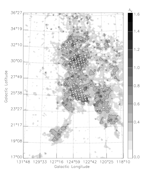
Figure 1: Visual extinction map of the Polaris Flare from $B$ star counts using the USNO-PMM catalogue. White crosses represent the DIRBE pixels used to compare the star count based extinction map with the SFD98 extinction map based on FIR emission

2.2 Comparison with SFD98

In Fig. 2, the ratio between SFD98 and star count extinction values is plotted against the dust temperature as derived by SFD98. For this we have smoothed both extinction maps to the DIRBE resolution. The DIRBE pixels used for this comparison are marked with white crosses in Fig. 1. The SFD98 $A_{V}$ values are systematically higher than those derived from star counts. The extinction ratio decreases for increasing dust temperatures. The mean ratio between the SFD98 and star count extinction values is 2.1. Fig. 3 shows the spatial distribution of the difference between SFD98 and our extinction map.

Figure 2: Comparison of the SFD98 extinction with star count extinction in the Polaris Flare versus the SFD98 temperature

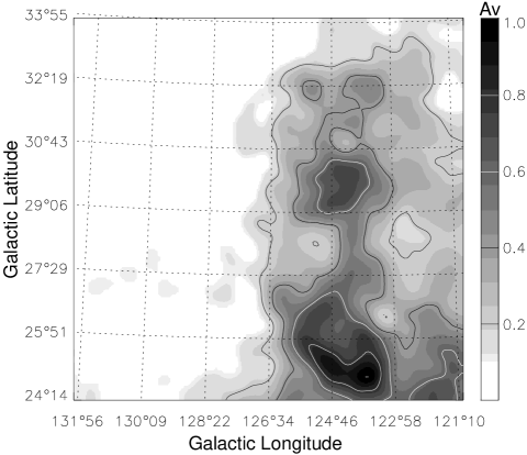
Figure 3: Difference between SFD98 and the star count extinction map at the DIRBE resolution. The two maps are in agreement outside the molecular cloud

The Polaris star counts raise a question about the validity of the SFD98 extinction map in regions of higher extinction that in those where they calibrated their conversion from FIR dust opacity to $A_{V}$. Previous studies have already pointed out similar discrepancies. Szomoru & Guhathakurta (1999) have presented a study of cirrus clouds with $UBVRI$ photometries and have compared their extinction derived from star counts, color excess, $UBV$ color–color diagrams and $BVI$ color–color diagrams. They found for their highest extinction cirrus, in Corona Australis, a discrepancy with the SFD98 map comparable to that found here for the Polaris Flare. Arce & Goodman (1999) have compared the extinction toward the Taurus cloud using four different techniques and they also concluded that the SFD98 map overestimates the extinction by a factor of 1.3-1.5. These results are confirmed by von Braun & Mateo (2001) who compared a color study of the globular cluster NGC 3201 ($b=8.6^{\circ}$) with the SFD98 extinction map for this line of sight. They concluded their analysis on a reddening overestimation in the SFD98 map.

2.3 Discussion

The extinction data presented in this paper together with similar data on other molecular clouds all lead to the same conclusion: the SFD98 extinctions are larger than the values derived from star counts in molecular clouds where $A_{V}\geq 1$ .

Cloud structure on angular scales smaller than the resolution of the star counts can make the measured $A_{V}$ smaller than the mean value of $A_{V}$. The relation between the mean extinction and the stellar density is not linear but logarithmic (Eq. 1) whereas the FIR integration over a cell is linear. This could thus explain the extinction discrepancy. Rossano (1980) has quantified this effect. Using his results, we found that a difference of a factor 2 for a visual extinction of 2 magnitudes would require a surface filling factor lower than 0.1. Such a low surface filling factor is incompatible with studies of the clumpiness of dust extinction which conclude on a smooth distribution of the dust in molecular clouds (Thoraval et al., 1997; Lada et al., 1999).

Another plausible explanation would be a shortcoming in the SFD98 dust temperature determination in molecular clouds which ignores temperature variation. This should be considered due to the coarse resolution of the SFD98 temperature map ($\sim 1^{\circ}$) compared to the clumpiness of the brightest structures in cirrus clouds. For example, for a given FIR brightness, an underestimation of the dust temperature translates into an overestimation of the dust opacity. Observations of molecular clouds at higher angular resolution than DIRBE do show temperatures locally lower than those of SFD98. For example, PRONAOS observations of a piece of the Polaris cirrus gave a dust temperature of 13.5 K (Bernard et al., 1999), significantly lower than the value of 16 K at the same position in the SFD98 temperature map. This example clearly shows that the SFD98 temperature is an effective temperature which represents a mean intensity value weighted over the dust seen within the solid angle of their study. The impact of the beam (and line-of-sight) averaging on the SFD98 temperatures and opacities can be discussed on the basis of a simple model where we assume that the emission comes from a mixture of two distinct components. In this calculation, we assume an emissivity law ($\propto\nu^{2}$) and fit a single black body to a combination of two black bodies at different temperatures. The effective optical depth is always smaller than the sum of the optical depth for the two temperatures. Thus if the $\tau_{\rm FIR}/A_{V}$ is the same for both dust components, our simple model shows that the SFD98 method always lead to an underestimation of $A_{V}$, the reverse of the discrepancy observed with star counts (Fig. 4). More generally, when a range of temperatures is present within the beam, the effective FIR dust opacity that is measured by SFD98 is always smaller than the mean opacity. Temperature variations within the beam thus cannot explain the extinction discrepancy between SFD98 and star counts.

The SFD98 map is a $\tau_{\rm FIR}$ map and not an $A_{V}$ map. To go from one to the other one needs to know the $\tau_{\rm FIR}/A_{V}$ ratio. We propose to explain the extinction discrepancy by variations in the $\tau_{\rm FIR}/A_{V}$ ratio between the low extinction regions used for the calibration of the $A_{V}$ and the Polaris molecular cirrus. Variations in the $R_{V}$ ratio from diffuse to dense clouds are interpreted as evidence for variations in the optical properties of large dust grains in molecular clouds (Cardelli et al., 1989). In our interpretation, the extinction discrepancy would thus be an additional signature of the evolution of dust from diffuse to dense clouds.

Figure 4: Effective to total optical depth ratio versus warm component fraction. Cold and warm components are described by the modified Planck function $P=B_{\nu}(T)\times(\lambda/\lambda_{0})^{-2}$ with $T_{\rm c}=13.5$ K and $T_{\rm w}=17.5$ K, respectively. Optical depths are derived by fitting each spectrum with a single modified Planck function.

3 Warm and cold dust components

3.1 Evidence for distinct emission components

The IRAS data have shown that no emission from aromatic hydrocarbons and very small grains at 12, 25 and 60 $\mu$m is seen towards the dense gas traced by the millimeter transitions of ¹³CO (Laureijs et al., 1991; Abergel et al., 1994). In practice, the molecular emission from this dense gas is observed to be well correlated with the difference between the 100 and 60 $\mu$m IRAS brightnesses. Lagache et al. (1998) combined the FIR DIRBE bands to the 60 $\mu$m data to separate along each line of sight the emission associated with the diffuse ISM and dense gas where both are present. With the long wavelength bands of DIRBE (100, 140 and 240 $\mu$m), they were able to determine a dust temperature for each of these two emission components. Their results show that the dust associated with the dense gas, as traced by the difference between the 100 and 60 $\mu$m brightness, is systematically colder ($T\sim 15$ K) than dust in the diffuse atomic interstellar medium ($T\sim 17.5$ K). We refer to these two emission components as cold and warm. The distinction between cold and warm emission components characterized by different dust temperatures and the abundance of small grains emission is corroborated by sub-mm observations at higher angular resolution for which the spatial separation of the infrared emission from diffuse and dense gas is easier to distinguish than with the DIRBE data (Bernard et al., 1999; Stepnik et al., 2001; Laureijs et al., 1996).

We propose to relate the extinction discrepancy to a variation in the $\tau_{\rm FIR}/A_{V}$ ratio between the cold and warm dust components. In their analysis of the DIRBE data, SFD98 did not consider the possible presence of distinct emission components with different dust temperature along the line of sight. They assume that large grain properties are everywhere the same and consequently that the temperature variations are exclusively due to changes in dust heating. In the Lagache et al. (1998) description of the data, the observed variations in the dust effective emission temperature are to a large extent due to various degrees of mixing between the warm and cold components. In a second paper, Finkbeiner et al. (1999), the same authors as SFD98, showed the necessity of including a very cold emission component with $\rm T\sim 9K$ in their analysis to improve the fitting of the FIRAS data at long wavelengths. However, this very cold component and the cold component of Lagache et al. (1998) are distinct (Note that they are not mutually exclusive and that both may be required to correctly describe the data). The cold component, derived from DIRBE data, is spatially correlated with known molecular clouds; the very cold component, deduced from FIRAS long-wavelength spectra is, on the contrary, present in all directions. For the subject of this paper the key difference between both components is that in the Finkbeiner et al. (1999) analysis the very cold component accounts for a fixed fraction of the emission, independent of sky position (fixed opacity ratios between the very cold and warm components, with temperature given by a power law) while in the Lagache et al. (1998) analysis the cold fraction varies spatially and is zero in the high latitude regions used by SFD98 for the calibration of the $\tau_{\rm FIR}/A_{V}$ ratio. Due to this spatial dependence, a difference in dust properties between the cold and warm emission components, namely in the $\tau_{\rm FIR}/A_{V}$ ratio, will limit the domain of the SFD98 conversion of $\tau_{\rm FIR}$ into $A_{V}$ and could account for the observed discrepancy with star counts. This statement is quantified in the following sections.

3.2 Separation of the warm and cold components

A separation of the warm and cold contributions to the infrared brightness is necessary in order to derive a temperature and FIR opacity for each component. To do this, we apply a method similar to that of Lagache et al. (1998) to DIRBE images of the Polaris Flare. Let $I(\lambda)$ ($\lambda$=100, 140, 240 $\mu$m) be the DIRBE emission at 100, 140 and 240 $\mu$m respectively, and $R(\lambda,60)$ the $I_{\nu}(\lambda)/I_{\nu}(60)$ flux ratio observed in cirrus clouds. The cold maps are computed at each wavelength according to the relationship: $I(\lambda)_{\rm c}=I(\lambda)-R(\lambda,60)\times I(60)$.

We first determine $R(100,60)$ using the correlation diagram of the diffuse cirrus emission around the Polaris cloud. We obtain $R(100,60)=4.0\pm 0.3$. At 140 and 240 $\mu$m the correlation diagrams are much more noisy. Therefore we prefer to compute $R(140,60)$ and $R(240,60)$ using $R(100,60)$ and assuming a large grain temperature of 17.5$\pm$0.5 K. We thus obtain: $R(140,60)=7.9\pm 1.1$ and $R(240,60)=6.4\pm 1.4$.

The produced cold maps have non-zero emission at a large scale due to 1) zodiacal residual emission (mainly coming from the 60 $\mu$m map) and 2) non-correction of the Cosmic Infrared Background. Therefore, under the assumption that the cold dust is distributed with limited angular extent in molecular clouds, we remove the low frequency structures using a $18\degr\times 18\degr$ median filter. We thus obtain, at the end, maps of cold dust emission at 100, 140, and 240 $\mu$m which are clumped on scales smaller than our filter size.

Map of statistical uncertainties for the cold emission are computed using the DIRBE release error maps:

$$\Delta_{\mathrm{sta}}I_{\nu}(\lambda)_{\rm c}=\sqrt{\Delta I_{\nu}(\lambda)^{2}+R(\lambda,60)^{2}\times\Delta I_{\nu}(60)^{2}}$$ (3)

Systematic uncertainties are derived following:

$$\Delta_{\mathrm{sys}}I_{\nu}(\lambda)_{\rm c}=\Delta R(\lambda,60)\times I_{\nu}(60)$$ (4)

Temperatures and optical depths are derived only for pixels containing significant cold emission (see Fig. 1), i.e. cold intensities at 100, 140 and 240 $\mu$m greater than 3$\sigma$, $\sigma$ being estimated at each wavelength using the width of the histograms of the cold emission maps.

Statistical and systematic uncertainties on the cold dust temperature and optical depth are computed using the statistical and systematic 100, 140 and 240 $\mu$m error maps of cold emission, respectively. Temperatures and optical depths are derived using the $\chi^{2}$ fitting and assuming a FIR dust emissivity index of 2. Uncertainties given by the $\chi^{2}$ fitting correspond to the 68.3% confidence level.

To determine the warm optical depth, we adopt the following method. We first remove to the 100 $\mu$m map the cold 100 $\mu$m emission and the cosmic FIR background value from Lagache et al. (2000). We then assume that the warm component has a temperature of 17.5$\pm$0.5 K with a FIR dust emissivity index of 2. Optical depth is thus directly proportional to the 100 $\mu$m warm emission.

The error on the warm emission, including both the systematic and statistical errors, is:

$$\Delta I_{\nu}(100)_{\rm w}=\sqrt{\Delta I_{\nu}(100)^{2}+\Delta I_{\nu}(100)_{\rm c}^{2}+\Delta I_{\nu}(100)_{\rm CIB}^{2}}$$ (5)

Optical depth uncertainties correspond to the minimum and maximum optical depth value allowed by the combination of $\Delta I_{\nu}(100)_{\rm w}$ and the 0.5 K error on the assumed dust temperature.

3.3 From far–infrared optical depth to visible extinction

Within the two components model, the total extinction can be written as the sum of the extinction in the warm and in the cold components:

$$A_{V}=A_{V}^{\rm w}+A_{V}^{\rm c}$$ (6)

and we have:

$$A_{V}^{\rm w}=\tau_{100}^{\rm w}\times\left(\frac{\tau_{100}}{A_{V}}\right)_{\!\!\rm w}^{-1}$$ (7)

$$A_{V}^{\rm c}=\tau_{100}^{\rm c}\times\left(\frac{\tau_{100}}{A_{V}}\right)_{\!\!{\rm c}}^{-1}$$ (8)

where the ratio $(\tau_{100}/A_{V})_{\rm w,c}$ are the emissivities of the dust at 100 $\mu$m for the warm and cold components, respectively. We take for the FIR-to-visible opacity ratio of the warm component, $(\tau_{100}/A_{V})_{\rm w}$, the ratio measured by SFD98 in low extinction regions. Then, we can derive $A_{V}^{\rm w}$ using Eq. 7 and the emissivity of the cold component is:

$$\left(\frac{\tau_{100}}{A_{V}}\right)_{\!\!\rm c}=\frac{\tau_{100}^{\rm c}}{A_{V}-A_{V}^{\rm w}}$$ (9)

3.4 Far–infrared emissivity of the warm component

The dust emissivity for the warm component is taken from SFD98. In their paper, they provide the value of $p=E_{B-V}/I_{100}=0.0184$, where $I_{100}$ is the 100 $\mu$m brightness expressed in MJy sr^-1 corrected from the zodiacal emission and scaled with the measured dust opacity from the pixel dependent dust temperature to a fixed temperature of 18.2 K. With this scaling, the conversion from $I_{100}$ to FIR opacity becomes pixel independent. We have:

$$\frac{\tau_{100}}{A_{V}}=\frac{I_{100}}{A_{V}\times\mathcal{B}_{100}(T)}=\frac{1}{R_{V}\,p\,\mathcal{B}_{100}(18.2\mathrm{K})}$$ (10)

For the mean Solar Neighborhood extinction law we have $R_{V}=A_{V}/E_{B-V}=3.1$. Moreover, a color correction should be applied to the optical depth because FIR fluxes are expressed for the effective filter wavelength assuming a $\nu^{-1}$ law. The correction consists of dividing the infrared flux by a color factor $\mathcal{K}$ defined in the DIRBE explanatory supplement as follow:

$${\cal K}=\frac{{\displaystyle\int_{\nu}}\left(\frac{I_{\nu}}{I_{\nu_{0}}}\right)_{\!\!\rm real}W_{\nu}\,d\nu}{{\displaystyle\int_{\nu}}\left(\frac{I_{\nu}}{I_{\nu_{0}}}\right)_{\!\!{\rm eff}}W_{\nu}\,d\nu}$$ (11)

where $W_{\nu}$ is the filter profile. The value given in the explanatory supplement is $\mathcal{K}_{100}(18.2K)=0.91125$.

Finally, the emissivity for the warm component is:

$$\left(\frac{\tau_{100}}{A_{V}}\right)_{\!\!\rm w}=\frac{{\cal K}_{100}(18.2\textrm{K})}{R_{V}\,p\,{\cal B}_{100}(18.2\textrm{K})}=1.31\,10^{-7}$$ (12)

3.5 Far–infrared emissivity of the cold component

3.5.1 Result

Following the procedure described in Sect. 3.2 and 3.3 we use the extinction map (Fig. 1) and the decomposition of the FIR flux in two components. We use the DIRBE resolution (the extinction map has been convolved by the DIRBE beam) and only pixels with high signal-to-noise ratio for both components.

Figure 5: Temperature and optical depth normalized at $1\mathrm{cm}^{-1}$ versus the galactic latitude for warm and cold components. Error bars represent the mean total uncertainty (statistical plus systematic) for each component

Fig. 5 show the temperature and the optical depth normalized to $1\mathrm{cm}^{-1}$ for the two components. The temperature in the Polaris Flare varies from 13 K to 15.5 K.

Figure 6: Emissivity variation versus temperature in the Polaris Flare, with the typical statistical (cross in the upper right corner) and systematic (squares) uncertainties. The filled square represents the SFD98 value which corresponds to the warm component emissivity. Dust emissivity of the cold component is 4.0 times larger than the warm one

Using Eq. 9 we obtain the values of the emissivity of the cold component, $\left(\frac{\tau_{100}}{A_{V}}\right)_{\!\!\rm c}$, presented in the Fig. 6. These values are all above the SFD98 value for the warm component (filled square in Fig. 6). The median value for the cold component emissivity at 100 $\mu$m is:

$$\left(\frac{\tau_{100}}{A_{V}}\right)_{\!\!\rm c}=5.3\,10^{-7}$$ (13)

This is 4.0 times larger than the SFD98 value for the warm component.

3.5.2 Uncertainties

In this sub-section, we compare uncertainties on the dust parameters with the dispersion of the points in Fig. 6. For the warm component, we are not able to separate the systematic from the statistical errors (see Eq. 5). Since these errors are small compared to those on the cold component parameters (by a factor of $\sim 3$) we focus on this last contribution to the observed scatter in Fig. 6.

Systematic errors.

In Sect. 3.2 we describe errors associated with the separation of the FIR flux in two components. Systematic errors on $\tau_{100}/A_{V}$ are dominated by uncertainties on $R(\lambda,60)$ which are used to derive the emission of the cold dust. These systematic errors would shift the whole set of data points. In Fig. 6 we give the direction and amplitude of these shifts for the median value. Extreme values for $\left(\frac{\tau_{100}}{A_{V}}\right)_{\!\!\rm c}$ are $3.6\,10^{-7}$ and $7.9\,10^{-7}$ and correspond to 2.7 and 6.0 respectively for the ratio of the emissivity between the two components. For $R_{V}=5.5$, we have already mentioned that star count extinction is multiplied by 1.12; the resulting median emissivity ratio would then be 3.1 (rather than 4.0).

Statistical errors.

The dispersion of the values represented in Fig. 6 suggests an increase of the FIR emissivity of the dust when the temperature decreases. However we examine the possibility of this trend being linked with statistical errors. In Fig. 6 the statistical errors are represented by error bars in the upper right corner. Since the optical depth is related to the FIR emission by the relation $\tau_{100}=I_{100}/\mathcal{B}_{100}(T)$, errors on the temperature and on the optical depth are correlated: temperature overestimation implies optical depth underestimation. This effect contributes to the observed dispersion in Fig. 6 but cannot fully explain its amplitude. We believe therefore that an intrinsic dispersion of the $\tau_{100}/A_{V}$ exists and that it may be related to an evolution of the emissivity with the temperature.

4 Discussion

4.1 Dust evolution from warm to cold component

The submillimeter analysis of the Polaris Flare by Bernard et al. (1999) has revealed an unexpected low temperature in this cirrus. They have used the extinction map of Fig. 1 to model the effect of the attenuation of the interstellar ultraviolet and visible radiation field on the dust temperature. They concluded that this cannot explain the observed temperature difference between Polaris and warm cirrus clouds. They thus suggest that the temperature difference is related to a change in optical dust properties. For a larger FIR to visible/UV extinction ratio, grains are able to radiate more efficiently the energy absorbed and thus their equilibrium temperature is reduced. Thereby, our interpretation of the extinction data is in agreement with Bernard et al. (1999) conclusions. A similar conclusion about the FIR dust emissivity is reached by the modeling of PRONAOS FIR/sub-mm observations of a molecular filament in Taurus (Stepnik et al., 2001). In this modeling, a change in the $\tau_{\rm FIR}/A_{V}$ ratio between the cold dust within the filament and the warm dust outside by a factor 3.4 is required to reproduce the brightness profiles across the filament at the various wavelengths. This study, unlike, ours does not rely on the empirical separation of warm and cold components.

The most straightforward explanation for the change in dust FIR emissivity between diffuse and molecular clouds is grain growth through grain-grain coagulation and accretion of gas species (e.g. Draine, 1985). These two processes should lead to composite grains with significant porosity. The effect of the formation of composite fluffy grains on the dust opacity is well explained by Dwek (1997). Two effects contribute to an increase in the dust opacity per unit dust mass. (1) The first contribution results from an increase in the effective grain sizes. For spherical grains of size $a$: $\tau_{\rm ext}=\pi a^{2}Q_{\rm ext}N_{d}$ where $N_{\rm d}$ is the dust column density and $Q_{\rm ext}$ the extinction efficiency, and $M_{\rm d}=4/3\pi a^{3}\rho N_{\rm d}$, where $\rho$ is the grain density. Within the Rayleigh limit ($2\pi a\ll\lambda$), $Q_{\rm ext}/a$ is independent of the grain size. For particles large relative to the wavelength ($2\pi a\gg\lambda$), it is $Q_{\rm ext}$ which is roughly size-independent. In practice, the Rayleigh limit applies to all grains in the FIR while the second limiting case applies to large interstellar grains ($a\sim 0.1\mu$m) in the UV. Within these limiting cases, one finds that $\tau_{\rm FIR}$ scales as $1/\rho$ while $\tau_{\rm UV}$ scales as $1/a\rho$. For increasing grain porosity, the effective grain density $\rho$ decreases and $\tau_{\rm FIR}$ increases. Thus, the ratio $\tau_{\rm FIR}/\tau_{\rm UV}$ scales as the grain size $a$. Qualitatively this also applies to the ratio $\tau_{\rm FIR}/A_{V}$. (2) The second, more subtle, effect is that the optical properties of the composite grains differ from the optical properties of their constituents: grain properties depend not only on their size but also on their composition and structure. In particular, the wavelength dependence of $Q_{\rm ext}/a$ changes with grain composition. For the specific case of composite carbon-silicate grains, this leads to a significant enhancement of the opacity in the FIR relative to that in the visible (Dwek, 1997). Dust properties of porous composite grains have also been quantified numerically (e.g. Bazell & Dwek, 1990; Mathis & Whiffen, 1989). In their work, Mathis & Whiffen (1989) show that it is possible to fit the extinction curve and its variations with $R_{V}$ with a size distribution of composite porous carbon+silicate grains. Their calculations show that enhancements of the $\tau_{\rm FIR}/A_{V}$ ratio by a factor of at least 3 can be obtained within the constraints set by the UV to near–infrared extinction curve.

The proposed interpretation of the variations in FIR dust emissivity implies that grain coagulation would be effective even within cirrus clouds and not only in dark clouds and proto-stellar condensations. Observed variations in the $R_{V}$ ratio have also been interpreted as evidence for grain growth from diffuse to dense clouds (e.g. Kim & Martin, 1996). It will thus be interesting to look for a plausible correlation between the changes in $\tau_{\rm FIR}/A_{V}$ and variations in the visible extinction curve. Note however that these two signatures of dust evolution from the diffuse ISM to molecular clouds are not necessarily correlated because $R_{V}$ and $\tau_{\rm FIR}/A_{V}$ do not share the same dependence on the dust porosity and size distribution (Mathis & Whiffen, 1989).

In the absence of multiband visible photometric data, we have no estimate of $R_{V}$ in the Polaris cloud and one can only make rather qualitative comments. Cardelli et al. (1989) have shown that the variations in the extinction curve from the UV to the near-UV, to a good approximation, can be related to one single parameter, $R_{V}$. The $R_{V}$-dependent extinction curves all converge in the near-IR but the change in the $\tau_{\rm FIR}/A_{V}$ ratio proposed to explain the extinction data is larger that one would expect from the simple extrapolation of this convergence to the FIR. For the Cardelli et al. relation, the $\tau_{\rm FIR}/A_{V}$ varies by a factor 1.2 for a large change in $R_{V}$ from 3.1 to 5.5. If we add the effect of such an $R_{V}$ change on the star count $A_{V}$ estimates (which needs to be multiplied by a factor 1.12 due to the fact that our star counts are based on a $B$ image, see section 2.1), the extinction discrepancy between SFD98 and star counts, a factor of about 2, is reduced by only a factor 1.34. This paper thus suggests that the $R_{V}$-dependent extinction curves should separate again in the FIR.

4.2 Validity of the SFD98 extinction map

We chose the Polaris Flare for its brightness in the cold emission map presented in Fig. 7. The white regions in this figure are the regions with cold emission, outside the Galactic plane, where the present work questions the validity of the SFD98.

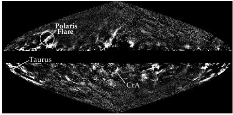
Figure 7: Cold component of the dust emission at 240 $\mu$m from Lagache et al. (1998)

As mentioned in Sect. 2.2, additional studies similar to the present work support our results (Szomoru & Guhathakurta, 1999; Arce & Goodman, 1999; von Braun & Mateo, 2001) for pieces of the Corona Australis and Taurus clouds. Both regions have an important cold emission in Fig. 7. Since the Szomoru & Guhathakurta (1999) work is a prelude to what can be done systematically with the Sloan Digitized Sky Survey (SDSS), it is crucial for further works to be aware that the dust emissivity varies in the FIR, even for cirrus cloud. Arce & Goodman (1999) suggest that the discrepancy results from a calibration bias. In the present paper we show that there is no general calibration that could be used in all directions. Optical properties of grains vary and the conversion from FIR fluxes to opacity cannot be limited to a single scaling factor.

For low galactic latitude ($|b|<10\degr$) it is obvious that the SFD98 map has to be used with caution since very different physical environments are mixed along the line of sight. Chen et al. (1999) propose a 3-dimensional extinction model to constrain the galactic structure based on the SFD98 map used toward globular clusters as close as 3° to the Galactic center. They found a recalibration was better to fit their data and they used the new calibration for the whole sky. The Galactic plane and even more, the Galactic center, are very complicated regions: the presence along the line of sight of massive stars which heat the interstellar dust and molecular clouds with cold dust makes impossible the separation of the different components which contribute to the FIR flux. It is not clear how their empirical calibration of the FIR emissivity can be related to those determined for the nearby interstellar medium.

Bianchi et al. (1999) have derived the FIR dust emissivity using wavelength dependences derived from FIR spectra of galactic emission and the SFD98 extinction map to normalize the $\tau_{\rm FIR}/A_{V}$ ratio. The authors admit that two components of temperature could exist at low galactic latitude but they omit that dust properties could also vary.

The knowledge of the extinction close to the Galactic plane is required to estimate precisely the properties of some objects, like the RR Lyrae type stars, used as a distance indicator. Stutz et al. (1999) used the SFD98 map to deredden RR Lyrae type stars in Baade’s window, i.e. 3° from the Galactic center.

5 Conclusion

We have presented an extinction map of the Polaris high latitude cloud derived from star counts. This extinction map is compared with that produced by SFD98 based on the IRAS and DIRBE FIR sky maps. Within the Polaris cirrus cloud, the SFD98 extinction value is found to be a factor 2 to 3 higher than the star count values.

We propose to relate the extinction discrepancy to variations in the $\tau_{\rm FIR}/A_{V}$ of interstellar dust from the warm and cold emission components introduced by Lagache et al. (1998) on the basis of the observed difference in small grain abundance and large grain temperature between the diffuse ISM and dense molecular gas. Within this interpretation, we find that the FIR emissivity of dust grains in the cold component is on average about 4.0 times (from 2.7 to 6.0) larger than it is in the warm component. There is a slight evidence that the evolution of the grain properties are gradual, in the sense that the $\tau_{\rm FIR}/A_{V}$ ratio increases when the cold dust temperature decreases. The increase in the FIR opacity could be tracing a growth of dust grains by coagulation. Our work is thus suggesting that the size/porosity of the large dust grains evolve within low opacity molecular cloud, such as the Polaris Flare.

SFD98 have converted the FIR opacity in extinction assuming a single emission temperature for each line of sight and $\tau_{\rm FIR}/A_{V}$ ratio. Our work questions the validity of this assumption in all regions with significant cold emission (Fig. 7). A few independent studies in other molecular clouds support this statement. The SFD98 extinction could be overestimating the true extinction in regions with cold emission that are found even at high Galactic latitude and for extinction as low as $A_{V}\gtrsim 0.5$. Variations in the dust emissivity preclude the conversion from FIR optical depth to $A_{V}$ with one single factor valid over the whole sky. Low latitude regions ($b<10^{\circ}$) and a small fraction of the high latitude sky require special attention.