New developments in the GALPROP CR propagation model

Abstract

The GALPROP cosmic-ray (CR) propagation model has been extended to three dimensions including the effects of stochastic SNR sources, a comprehensive cross-section database, and nuclear reaction networks. A brief description of the new code is given and some illustrative results for the distribution of CR protons presented. Results for electrons and $\gamma$-rays are given in an accompanying paper.

1 Introduction

We have previously described a numerical model for the Galaxy encompassing primary and secondary cosmic rays, $\gamma$-rays and synchrotron radiation in a common framework (Strong et al. 2000 and references therein). Up to recently our GALPROP code handled 2 spatial dimensions, $(R,z)$, together with particle momentum $p$. This was used as the basis for studies of CR reacceleration, the size of the halo, positrons, antiprotons, dark matter and the interpretation of diffuse continuum $\gamma$-rays.

Some aspects of the problem cannot be addressed in such a cylindrically symmetric model: for example the stochastic nature of the cosmic-ray sources in space and time, which is important for high-energy electrons with short cooling times, and local inhomogeneities in the gas density which can affect radioactive secondary/primary ratios.

In common with most other models it has been previously assumed that the CR source function can be taken as smooth and time-independent, an approximation justified by the long residence time ($>10^{7}$ years) of cosmic-rays in the Galaxy. However the inhomogeneities have observable consequences, and their inclusion is a step towards of the goal of a “realistic” propagation model based on Galactic structure and plausible source properties. The original motivation for this extension was to study the high-energy electrons, since the observation of the $>1$ GeV excess in the EGRET spectrum of the Galactic emission has been proposed to originate in inverse-Compton emission from a hard electron spectrum; this hypothesis can only be reconciled with the local directly-observed steep electron spectrum if there are large spatial variations which make the spectrum in our local region unrepresentative of the large-scale average.

Here we briefly describe an extension of the model to 3D, which can address these issues, and illustrate the results for protons. The new network and cross-sections is illustrated for B/C in the 2D case. The effect on electrons and $\gamma$-rays is presented in an accompanying paper (Strong and Moskalenko, ‘A 3D time-dependent model for cosmic rays and $\gamma$-rays’, these proceedings: hereinafter paper II).

2 Model

The GALPROP code, which solves the CR propagation equations on a grid, has been entirely rewritten in C++ using the experience gained from the original version and including both 2D and 3D spatial grid options. The 2D mode essentially duplicates the original version, with improved cross-section routines. In 3D $(x,y,z,p)$ the propagation is solved as before using a Crank-Nicolson scheme. The additional dimension considerably increases the computer resources required, but a 200 pc grid cell or finer is still practicable. As in the original version, the effects of diffusion, convection, diffusive reacceleration, and energy losses are included, each with adjustable parameters defined for a GALPROP run.

2.1 Cross-sections and reaction network

Cosmic-ray nuclear reaction networks are included with a comprehensive new cross-section database; this allows the models to be tuned on stable and radioactive CR secondary/primary ratios, in particular B/C and ¹⁰Be/⁹Be. The nuclear reaction network is built using the Nuclear Data Sheets. The isotopic cross section database consists of more than 2000 points collected from sources published in 1969–1999. This includes a critical re-evaluation of some data and cross checks. The isotopic cross sections for B/C were calculated using the authors’ fits to major beryllium and boron production cross sections C,N,O $\to$ Be,B. Other cross sections are calculated using the semi-phenomenological approximations by Webber et al. (1990) (code WNEWTR.FOR of 1993) and/or Silberberg and Tsao (code of 2000) renormalized to the data where it exists.

The reaction network is solved starting at the heaviest nuclei (i.e. ⁶⁴Ni). The propagation equation is solved, computing all the resulting secondary source functions, and then proceeds to the nuclei with $A-1$. The procedure is repeated down to $A=1$. In this way all secondary, tertiary etc. reactions are automatically accounted for. To be completely accurate for all isotopes, e.g. for some rare cases of $\beta^{\pm}$-decay, the whole loop is repeated twice. Our preliminary results for all cosmic ray species $Z\leq 28$ are given in Strong and Moskalenko (2001).

2.2 Stochastic sources

Another major enhancement is the inclusion of stochastic SNR events as sources of cosmic rays. The SNR are characterized by the mean time $t_{SNR}$ between events in a 1 kpc³ unit volume, and the time $t_{CR}$ during which an SNR actively produces CR.

The propagation is first carried out for a smooth distribution of sources to obtain the long timescale solution, using the fast technique described in Strong and Moskalenko (1998); then the stochastic sources are started and propagation followed for the last 10⁷ years or so with timesteps sufficiently fine (e.g., 10³ years) to resolve the SNR events and all propagation effects (see below for more details of the method). For high-energy (TeV) electrons which lose energy on timescales of 10⁵ years the effect is a very inhomogeneous distribution with consequences for diffuse $\gamma$-rays, as shown in the accompanying paper II. However also the protons (and other nuclei) show fluctuations which are strongly energy-dependent. The amplitude of the fluctuations of both electrons and nuclei depends on the parameters $t_{SNR}$ and $t_{CR}$. The time $t_{SNR}$ is adjusted to be consistent with estimates of the SNR rate (e.g., Dragicevich et al. 1999); models for shock acceleration in SNR indicate $10^{4}<t_{CR}<10^{5}$ yr, the sources switching off when they move from the adiabatic to the radiative phase (Sturner et al., 1997).

An additional advantage of the 3 spatial dimensions is that the gas distribution (for energy losses, secondary production and $\gamma$-rays) can be modelled in as much detail as required, based on current HI, CO, FIR, etc. surveys. Spiral structure and local inhomogeneities can be included if required. Global parameters such as the CR luminosity of the Galaxy, and hence the average SNR energy injection into CR, are also computed since they provide essential constraints (see paper II).

2.3 Extension to 3D

Since the solution in $(x,y,z,p)$ on a fine grid involves large arrays and many time-steps, the code has been made vectorizable so that it can benefit from the use of vector machines with a speed gain typically 100. This is only required for the final “stochastic SNR” part of the solution, since the “smooth” solution is fast enough on non-vector machines. In addition we have the option to make use of symmetry in the spatial dimension where it does not affect the application of the results (e.g., about $z=0$). This leads to an addition large gain in speed. Typical parameters are: grid size $\Delta x=\Delta y=\Delta z=200$ pc, Galaxy dimension 60 kpc $\times$ 60 kpc $\times$ 4 kpc, and energy range 1 MeV – 1 TeV on a logarithmic scale with factor 1.2.

3 CR Protons

For illustration we show results for a model with reacceleration based on Strong et al. (2000), and $t_{SNR}$ = 10⁴ yr corresponding to a Galactic rate of 3 SN/century. Fig. 1 shows the distribution of protons in the Galactic plane ($z=0$) for a representative quadrant, at various energies. The stochastic SNR source produce fluctuations, which are a minimum around 1 GeV and increase at low energies due to energy losses and at high energies where the storage of particles in the Galaxy is much reduced so that the effect of sources manifests itself on the distribution. Note that the nature of the fluctuations is different at low and high energies.

Fig. 2 shows a sample of proton spectra at different $(x,y)$ positions; the fluctuations are evident but much smaller than for electrons (paper II).

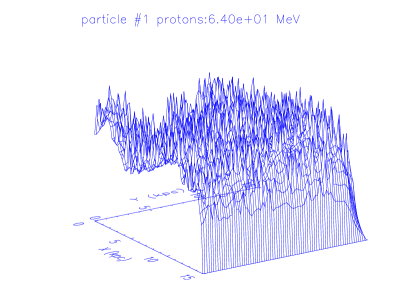
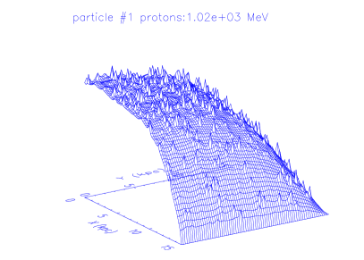
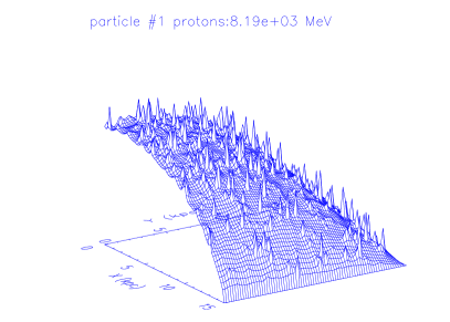
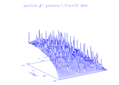
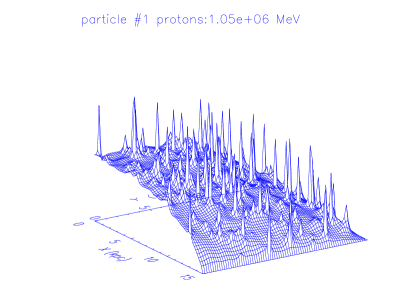
Figure 1: Flux of protons with E= 64 MeV, 1 GeV, 8.2 GeV, 130 GeV, and 1 TeV (left to right, top to bottom) at $z=0$, for $t_{SNR}$ = 10⁴ yr.

The fluctuations in the GeV nuclei will have some effect on the $\pi^{0}$-decay diffuse $\gamma$-ray emission above 100 MeV, but the variations will be small compared to the inverse Compton component since the GeV nuclei variations are much smaller than for the TeV electrons responsible for GeV $\gamma$-rays via IC (see paper II). Above 100 GeV $\gamma$-ray energies however the effect on the $\pi^{0}$-decay component will be larger, and should be detectable for example by the GLAST mission.

Figure 2: Sample proton spectra for various $x,y$ at $z=0$, illustrating the variations of shape with position. Model as Fig. 1.

Figure 3: B/C ratio as calculated for a model with reacceleration using the new reaction network and cross-sections. Lower curve: interstellar, upper curve: modulated for 450 MV. Data: see Strong and Moskalenko (2001).

4 Secondary/primary ratio

We illustrate the new cross-sections and network with the B/C ratio (Fig. 3) for the case of the same model (with reacceleration) as for electrons. More details of the application to nuclei can be found in Strong and Moskalenko (2001) and Moskalenko et al. ‘New calculation of radioactive secondaries in cosmic rays’ (these proceedings) and to antiprotons in Moskalenko et al. ‘Secondary antiprotons in cosmic rays’ (these proceedings).

5 Conclusion

This paper is intended only as an illustration of the possibilities opened up with such a 3D code. Future work will concentrate on the effect of inhomogeneities in the gas distribution (e.g., the local bubble) on radioactive CR nuclei, as well as implications for electrons and $\gamma$-rays.