Making Maps Of The Cosmic Microwave Background:
The maxima Example.

Abstract

This work describes Cosmic Microwave Background (CMB) data analysis algorithms and their implementations, developed to produce a pixelized map of the sky and a corresponding pixel-pixel noise correlation matrix from time ordered data for a CMB mapping experiment. We discuss in turn algorithms for estimating noise properties from the time ordered data, techniques for manipulating the time ordered data, and a number of variants of the maximum likelihood map-making procedure. We pay particular attention to issues pertinent to real CMB data, and present ways of incorporating them within the framework of maximum likelihood map-making. Making a map of the sky is shown to be not only an intermediate step rendering an image of the sky, but also an important diagnostic stage, when tests for and/or removal of systematic effects can efficiently be performed. The case under study is the maxima-i data set. However, the methods discussed are expected to be applicable to the analysis of other current and forthcoming CMB experiments.

I Introduction

This paper presents a comprehensive set of data analysis methods aiming at the production of a map of the sky and an accurate estimate of map uncertainty in a case of CMB mapping experiments. We describe a variety of maximum-likelihood-based map-making methods, and discuss their performance in the analysis of the maxima-i data set.

maxima is a balloon-borne experiment Lee1999 built primarily in Berkeley Maxima and designed to make a number of short-duration flights. To date the maxima team has published the results of the first flight of the instrument Hanany2000 ; Lee2001 , consisting of a high-resolution map of almost $100$ square degrees of the microwave sky, together with a power spectrum of the CMB anisotropies observed in the map covering a broad range in $\ell$ space from $\ell\sim 35$ up to $\sim 1235,$ corresponding to angular scales from $5$ degrees down to $5$ arcminutes. Such products are final results of an involved data analysis pipeline described in this paper. The complexity and size of this data set have proven to be a significant challenge for data analysis methods setting demanding requirements for both their precision and speed. The challenge which our methods and tools are designed to meet. With other complex and advanced CMB experiments in progress and anticipated (including the satellite missions, MAP Map and Planck Planck ), these tools and methods can be expected to be of wider interest and applicability. Describing the details of the maxima-i data analysis is another goal of this paper.

The structure of this work is as follows; in Sect. II we deal with the data in the time domain, focusing on data pre-processing and noise estimation, including an outline of the basic features of the maxima-i data set, and of the simulation tools used to test our map-making pipeline. Sect. III is devoted to the description and comparison of a suite of different map-making methods. Those simultaneously produce both a map and a corresponding pixel-pixel noise correlation matrix. Although the algorithms are all based on the maximum likelihood approach, they differ in the way they attempt to optimize the balance between accuracy and speed. We demonstrate their performance in analyzing maxima-like simulations as well as the actual maxima-i data set. In Sect. IV we discuss ways of handling systematic effects within the general framework of maximum likelihood map-making. Although such systematics are inevitable in real CMB data sets, they are rarely considered in more theoretical accounts of CMB data analysis (e.g.,  Wright1996a ; Tegmark1997maps ; Tegmark1997design ; Oh1999 ; Ferreira2000 ; Stompor2000 ; Hinshaw2000 ; Dore2001a ; Natoli2001 ). In Sect. V we combine these elements, and consider some practical aspects of recently-proposed iterative algorithms for time-domain noise estimation Ferreira2000 ; Prunet2000 . In Sect. VI, we complete our presentation with a description of the numerical tests we have developed to check consistency of our analysis.

The inter-dependencies of different sections of this paper are depicted in Fig. 1.

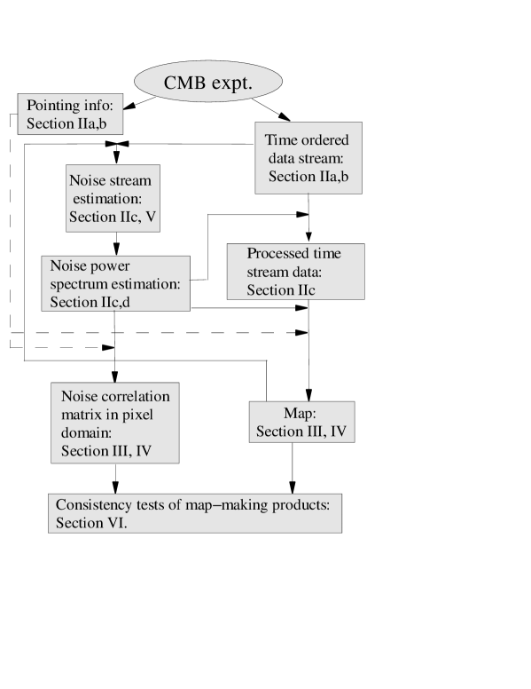
Figure 1: A flow-chart showing the layout and inter-dependencies of the sections of this paper, as well as mutual relations of different stages of the data analysis pipeline as described in the text.

Table 1: A summary of the notation used in this paper.

Symbol	Description	Section
$\Delta$	data sampling interval	II.1
${\hbox{\boldmath$d$\unboldmath}}(t)$	time stream data	II.2
${\hbox{\boldmath$d_{F}$\unboldmath}}(t)$	time stream data convolved with filter $F$	II.2
$F$	instrumental filters (all together)	II.2
$F_{low}$	AC low-pass electronic filter	II.2
$F_{high}$	AC high-pass electronic filter	II.2
$F_{bolo}$	bolometer low-pass filter	II.2
${\hbox{\boldmath$t$\unboldmath}}_{sky}$	sky signal	II.2
${\hbox{\boldmath$x$\unboldmath}}\left({\hbox{\boldmath$\alpha$\unboldmath}}\right)$	$\alpha$-synchronous signal	II.2
$n_{t}$	time stream noise	II.2
$P\left(f\right)$	time domain noise power spectrum	II.2
$P_{W}\left(f\right)$	prewhitened time domain noise spectrum	II.3
$W$	prewhitening filter	II.3
$\lambda_{c}$	noise correlation length in time domain	II.3
$S\left(f\right)$	spectrum smoothing window function	II.4
$N_{t}$	time domain noise correlation matrix	II.4
$N_{Ct}$	circulant part of $N_{t}$	II.4
$N_{St}$	sparse part of $N_{t}$	III.3
$A$	pointing matrix of the experiment	III.1
$m_{p}$	pixelized sky $\equiv$ map	III.1
$N_{p}$	noise correlation matrix in pixel domain	III.1
$N_{Cp}$	circulant part of $N_{p}$	III.3
$N_{Sp}$	sparse part of $N_{p}$	III.3
$n_{pix}$	number of pixels in a map $m_{p}$	III.1
$n_{s}$	length of the time stream segment	III.1
${\hbox{\boldmath$B$\unboldmath}},{\cal B}$	pointing matrices of synchronous effects	IV.1
$x_{q}$	extra fictitious pixels	IV.1
${\cal A}$	generalized pointing matrix	IV.1
$\hat{m}_{p}$	generalized map	IV.1
${\cal N}$	generalized noise correlation matrix	IV.1
$\tau_{t}$	time domain template	IV.2
$\delta^{K}$	Kronecker delta	IV.2
$u_{p}$	vector of ones	IV.3
$v_{p}$	singular pixel domain eigen-vector	IV.3, IV.4
$C_{\ell}$	CMB anisotropy power spectrum	IV.3, IV.6
$M_{p}$	total signal+noise correlation matrix	IV.3, IV.6
${\hbox{\boldmath$S_{p}$\unboldmath}}\left(C_{\ell}\right)$	CMB signal correlation matrix	IV.3, IV.6
${\hbox{\boldmath$N_{p}$\unboldmath}}^{-{1/2}}$	Cholesky factor of matrix $N_{p}$	III.4, VI
$w_{p}$	decorrelated map	VI

In this paper we do not consider issues related to the subsequent statistical investigation of these maps, such as tests for Gaussianity or power spectrum estimation. Our map-making methods are intended to be as general as possible, and because they provide both a map and a pixel-domain noise correlation matrix, they do not restrict the subsequent choice of statistical tool. Methods for obtaining an angular power spectrum from, or for searching for non-Gaussianity in, such maps have been described in a number of recent papers (e.g., Tegmark1997pow ; BJK1998 ; Borrill1999pow ; Szapudi2000 ; pseudcl ; Dore2001b ; Hivon2001 and FMG98 ; Wu2000 ; Wu2001b ; Cayon2001 , respectively). The power spectra shown in this paper have been computed using a generic uncustomized version of a quadratic estimator as implemented in the publicly-available MADCAP package Madcap ; Borrill1999mad .

A comprehensive discussion of the maps and power spectra produced by the maxima-i experiment can be found elsewhere Hanany2000 ; Lee2001 ; Stompor2001b ; their cosmological implications are discussed in Stompor2001a ; Balbi2000 ; Wu2001b .

Hereafter, we denote vectors and scalars with bold and non-bold lower case letters (either Roman or Greek) respectively, while matrices and operators are denoted with either bold or caligraphic upper case letters. Vector and matrix components are indexed in parentheses, rather than by subscript; subscripts and superscripts are used to distinguish between different variants of a given quantity, e.g., $p$ and $t$ denote a pixel and a time domain quantity respectively. A tilde over a quantity denotes its Fourier transform, i.e.,

$${{\hbox{\boldmath$\tilde{g}$\unboldmath}}}\left(f\right)\equiv\int dt\,{\hbox{\boldmath$g$\unboldmath}}\left(t\right)\exp\left(2\pi\iota ft\right).$$

Occasional failures of these good intentions are also acknowledged. A summary of the most frequently used symbols is given in Table 1.

II Time ordered data

II.1 The maxima-i data set

The maxima-i data and instrument have been described in Lee1999 ; Hanany2000 ; Lee2001 . The maxima-i data set consists of approximately $2,300,000$ measurements for each of 16 photometers and 4 dark channels used to monitor the experiment. To date only data from six of the detectors have been analyzed. These include four photometers sensitive to CMB photons (3 with frequency bandwidths centered on $150$ GHz and 1 on $240$ GHz), one photometer monitoring atmosphere and foregrounds at $410$ GHz, and one ‘dark’ bolometer (screened from incident photons) used to search for systematic problems. Each of the data streams for each of these detectors is divided into two parts, hereafter called the CMB1 and CMB2 scans respectively (see Fig. 2). These scans were taken at different elevations and were separated in time by $\sim 1.5$ hours. Projected on the sky, they largely overlap one another, creating a well-crosslinked map. Each of the two scans is further subdivided into 11 (CMB1 scan) and 10 (CMB2 scan) data subsets whose lengths range from $30,000$ to $250,000$ time samples. These disjoint stretches of contiguous data – hereafter referred to as time stream segments – are defined by the requirement that the noise within a segment be approximately stationary. The noise correlations between the segments are guaranteed to be negligible by discarding a sufficiently long section of the time stream data between neighboring segments. In addition, each of the segments has an overall offset and gradient subtracted independently.

Not all measurements within a segment are to be included in the further analysis. Measurements compromised by glitches – cosmic rays hits, telemetry drop-outs, or other short transients – are flagged as ’bad’ and constitute gaps in a segment. We usually determine about $2-3\%$ of the time samples as gaps.

The signal and noise are subjected to several filters before being recorded, including a low-pass filter due to the detector time constant and subsequent AC low- and high-pass filters in the readout electronics. These filters are phase-shifting (i.e., their Fourier space representation is by complex numbers) and they define the temporal frequency response of the instrument to a band between $f\lower 2.15277pt\hbox{$\;\buildrel>\over{\sim}\;$}0.01$Hz and $f\lower 2.15277pt\hbox{$\;\buildrel<\over{\sim}\;$}20$Hz. This frequency response together with the scan strategy give maxima-i sensitivity to the sky features in the range of angular scales from $\sim 5$ degrees down to $\sim 5$ arcminutes. The instrumental filters must be deconvolved from the time ordered data in the course of the data analysis. The functional form of the electronic filters is accurately measured in the laboratory. The detector time constant is measured using the in-flight response of the detectors to a known source – in the case of maxima-i, Jupiter. For our purposes here it is assumed that the instrumental filters are known to a negligible uncertainty in the range of frequencies of interest, i.e., $\lower 2.15277pt\hbox{$\;\buildrel<\over{\sim}\;$}50$Hz. (Note that the bolometer time constant has an uncertainty of $\sim 0.5-1.0$ ms. This error is included in the analysis of the maxima-i data Hanany2000 ; Lee2001 ; Stompor2001b , but we neglect it for the purpose of this paper.) The data sampling interval is fixed throughout the entire observation at $\Delta=0.0048$ s. Hereafter, we identify an observation in the time domain (including gaps) by a global sample-number index.

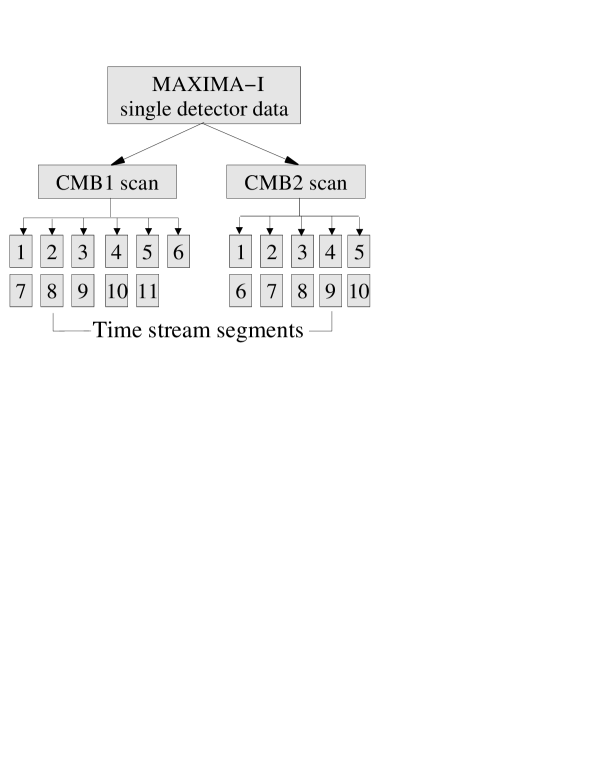
Figure 2: A structure of the maxima-i data set.

The maxima scanning strategy includes an azimuthal primary mirror chop with a frequency $\sim 0.45$ Hz superimposed on a slow azimuthal balloon gondola oscillation with a characteristic frequency of $\sim 0.01$ Hz. Both the position of the primary mirror with respect to the gondola and the azimuthal position of the gondola were recorded during flight, enabling the tracking of primary mirror and/or gondola synchronous systematic effects.

The maxima pointing is reconstructed using the observations of guide stars made throughout the flight. With an rms accuracy better than $\sim 1^{\prime}$, pointing uncertainty is neglected during the map-making stage, although it can, and indeed should, be included as a systematic uncertainty of the final power spectrum (e.g., Lee2001 ).

The time stream data are assigned to pixels prior to map-making. The relatively small angular size of the sky patch observed by maxima-i allows us to use simple square pixels on a grid whose rows are at constant declination. Due to computational constraints, most of the tests discussed in this paper have been performed using 8 arcminute pixels, although the highest resolution maxima-i results have been computed using 3 arcminute pixels  Lee2001 .

The independence of a pixel’s size on its sky position enables us to account for the extra smoothing due to the pixelization by using a simple, albeit approximate, pixel window function Wu2001a . This approximation usually breaks down at the smallest angular scales, due to the lack of uniformity of the sky sampling on these scales. Ways of alleviating this problem are discussed elsewhere Lee2001 . The methods discussed below are independent of the assumed pixelization scheme.

II.2 Time stream modeling and simulations

Drawing from the maxima-i experience, we now explicitly list all the features of the time stream data which we have found to be important in the data analysis. We also briefly explain how we incorporate these features into our simulations, which are then used for tests of our data analysis tools.

II.2.1 Time stream model

We denote the entire raw time stream from a single detector, including the effect of the instrumental filters, as $d_{F}$. As noted above, this is subdivided into a number ($n_{seg}$) of disjoint segments, so that we can write ${\hbox{\boldmath$d_{F}$\unboldmath}}\equiv\bigcup_{I=1}^{n_{seg}}{\hbox{\boldmath$d^{I}_{F}$\unboldmath}}$.

Every measurement contains contributions from both the sky and the instrument, and is modeled as,

$${\hbox{\boldmath$d_{F}^{I}$\unboldmath}}\left(i\right)=\sum_{j}{\hbox{\boldmath$F$\unboldmath}}\left(i,j\right)\left[{\hbox{\boldmath$t$\unboldmath}}_{sky}\left({\hbox{\boldmath$\gamma$\unboldmath}}\left(j\right)\right)+{\hbox{\boldmath$x$\unboldmath}}\left({\hbox{\boldmath$\alpha$\unboldmath}}\left(j\right)\right)\right]+{\hbox{\boldmath$n_{t}$\unboldmath}}\left(i\right).$$ (1)

$F$ denotes the effect of all of the instrumental filters, and for maxima is therefore a convolution of three filters – ${\hbox{\boldmath$F$\unboldmath}}\equiv{\hbox{\boldmath$F_{high}$\unboldmath}}\star{\hbox{\boldmath$F_{low}$\unboldmath}}\star{\hbox{\boldmath$F_{bolo}$\unboldmath}}$ – corresponding to the AC high-pass, AC low-pass, and bolometer low-pass filters. ${\hbox{\boldmath$t$\unboldmath}}_{sky}\left({\hbox{\boldmath$\gamma$\unboldmath}}\left(i\right)\right)$ is the temperature of the sky in the direction ${\hbox{\boldmath$\gamma$\unboldmath}}\left(i\right)$ observed at time $i$. $x$ is any extra systematic ‘$\alpha$-synchronous’ effect (e.g., primary mirror chop synchronous noise) which only depends on a known parameter $\alpha$ (e.g., the mirror position). The dependence of $x\left(\alpha\right)$ on time is, therefore, exclusively a result of the time-dependence of the parameter $\alpha$. ${\hbox{\boldmath$n_{t}$\unboldmath}}\left(i\right)$ denotes the total (Gaussian, correlated) instrument noise in observation $i$. In fact, independent noise components are introduced into the time stream at four different stages in the instrument and, more precisely, the total noise is represented as

$${\hbox{\boldmath$n_{t}$\unboldmath}}={\hbox{\boldmath$F_{high}$\unboldmath}}\left[{\hbox{\boldmath$F_{low}$\unboldmath}}\left[{\hbox{\boldmath$F_{bolo}$\unboldmath}}{\hbox{\boldmath$n_{t1}$\unboldmath}}+{\hbox{\boldmath$n_{t2}$\unboldmath}}\right]+{\hbox{\boldmath$n_{t3}$\unboldmath}}\right]+{\hbox{\boldmath$n_{t4}$\unboldmath}}.$$ (2)

Here ${\hbox{\boldmath$n_{t1}$\unboldmath}},$ ${\hbox{\boldmath$n_{t2}$\unboldmath}},$ $n_{t3}$ and $n_{t4}$ denote the independent noise components added to the signal prior to the bolometer low-pass, AC high-pass, AC low-pass filtering, and signal digitization, respectively. $n_{t1}$ and $n_{t2}$ components together are expected to dominate the total instrumental noise with only $n_{t1}$ component displaying a $1/f$ behavior at low frequencies attributable to temperature fluctuations of the detector. Though all such features are of importance for proper forecasting and simulations of a performance of an experiment, none of these needs to be assumed in the noise estimation described in Sect. II.3, which directly estimates the total noise, $n_{t}$. The instrumental noise is assumed to be Gaussian and stationary within each segment, and is described by a (segment-dependent) noise power spectrum, $P\left(f\right)$. Each segment is assumed to consist of measurements evenly spaced in time. However, the data constituting gaps are not to be included in a final map.

II.2.2 Simulations

In order to test our data analysis pipeline we want to be able to simulate the time stream of a maxima-i like experiment. The simulation is designed to incorporate all the important features of the actual data set listed above, including the gap and segment structure, scanning strategy, and an approximate (symmetric) beam Wu2001a .

The simulated time stream is described by Eq. (1). The sky signal ($t_{sky}$) is generated by applying the known pointing solution to a simulated CMB sky, generated as a high-resolution Gaussian realization given some fiducial cosmological parameters. We also include a primary mirror chop synchronous systematic effect, $x\left(\alpha\right)$, in our simulations, varying both its functional dependence on the primary mirror position and its amplitude. The instrumental filters are then applied to the simulated time stream as described by Eq. (1). Their functional form follows that of actual maxima filters.

Finally we add Gaussian correlated noise to each time sample. This is modeled according to Eq. (2) assuming that each component, $n_{ti}$, has a power spectrum in a form given by,

$$P_{sims}\left(f\right)=\sigma_{sims}^{2}\left(1+\frac{f_{knee}}{f}\right).$$ (3)

This approach means that our simulations mimic the range of floating point operations required in analyzing the real data, giving us some insight into possible numerical error accumulation in our data analysis pipeline.

II.3 Time stream processing and noise estimation

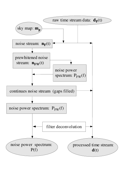
Figure 3: A flow-chart of the noise estimation procedure outlined in Sect. II.3. Objects inscribed in ovals are either input or output products of the procedure. This procedure can be incorporated as a part of the iterative noise estimation as described in Sect. V. In this case, its products (noise power spectrum and a processed time stream) are used to generate a sky map, which is one of input objects as shown in this chart.

We now describe the procedure for simultaneously estimating the time-domain noise power spectrum and restoring the stationarity of time stream noise by re-filling the flagged-data gaps in the time stream.

Typically, map-making methodologies assume that the time-domain noise power spectrum is precisely known, even though in practice it has to be estimated from the time stream data itself. The error in this estimation is therefore not included in general in the end-to-end data analysis error budget (although see Ferreira2000 for a possible way of tackling this issue). This fact clearly highlights the need for a high level of precision at this stage.

Figure 4: Filters used in the analysis of maxima-i data. Left panel shows a frequency domain representation of the filters. Thin solid and dashed lines show the (absolute values of) real and imaginary parts of the total instrumental filter, $\widetilde{F}\left(f\right)$, and the thick line its complex amplitude, $|\widetilde{F}\left(f\right)|$. The dot-dashed line depicts the real prewhitening filter, $\widetilde{W}\left(f\right)$, as defined in Eq. (7) ($2\beta=1.0$). The time domain representation of these filters shown in middle panel: solid line - total instrumental filter and dashed line its amplitude; and right panel - the prewhitening filter. The effective time domain widths of these filters assumed in the analysis are 100 time samples for both instrumental filters and 50 time samples for the prewhitening filter.

The time stream model described by Eq. (1) is quite complex. Some of its features are of less importance for this Section so, for simplicity, we start by assuming that the time stream data contains only Gaussian noise (i.e., no sky or systematic signals, ${\hbox{\boldmath$t_{sky}$\unboldmath}},{\hbox{\boldmath$x$\unboldmath}}\ll{\hbox{\boldmath$n_{t}$\unboldmath}}$) and focus on resolving problems in the noise estimation arising from the presence of gaps in the time stream and of noise correlations on time scales comparable to the length of an entire data segment.

The presence of discontinuities (gaps) in the time stream poses a two-fold problem. It is an obstacle both to estimating the time stream noise spectrum and to devising a fast and efficient map making algorithm (see Sect. III). It is therefore desirable to restore time stream continuity without compromising the stationarity of the noise or sacrificing too much of the data. These two goals, estimating the noise power spectrum and restoring the continuity of the time stream, are achieved by a procedure described below (see Fig. 3 for its synopsis).

II.3.1 A pure noise time stream

The initial input at this stage consists of the time stream data with the instrumental filters convolved, $d_{F}$. The filters can be deconvolved in the frequency domain,

$${\hbox{\boldmath$d$\unboldmath}}\left(t\right)=\int df\,{{\hbox{\boldmath$\tilde{d}_{F}$\unboldmath}}}\left(f\right)\widetilde{F}^{-1}\left(f\right)\exp\left(-2\pi\iota ft\right).$$ (4)

This deconvolution could be done immediately, prior to any further time stream manipulation, but this is not recommended due to the high-frequency noise it adds to the time stream (see Figs. 4 & 5). Although this noise would not be a problem for our formalism in theory, it can be a source of significant numerical error in any practical implementation, possibly biasing the final results. This numerical error is usually incurred while Fourier transforming the noise power spectrum. Instrumental filter deconvolution causes the noise power at the highest frequencies to dominate the total power of the time stream noise by many orders of magnitude, and consequently a small error in the total noise power estimate translates into a substantial error in the noise power estimate in the lower range of frequencies of most interest. The remedy is either to leave the instrumental filter deconvolution until after the noise estimation stage, or to perform the deconvolution at the beginning but concurrently convolving an extra (real) filter, $\widetilde{X}_{re}(f)$, to suppress the high frequency noise, i.e.,

$${\hbox{\boldmath$d$\unboldmath}}\left(t\right)=\int df\,{{\hbox{\boldmath$\tilde{d}_{F}$\unboldmath}}}\left(f\right)\widetilde{X}_{re}\left(f\right)\widetilde{F}^{-1}\left(f\right)\exp\left(-2\pi\iota ft\right).$$ (5)

In this case, a conventional choice is to apply a real filter given in the frequency domain as the amplitude of the total instrumental filter, i.e., $\widetilde{X}_{re}\left(f\right)=\left|\widetilde{F}\left(f\right)\right|$. In some map-making algorithms this filter can be deconvolved from the time stream data once the noise power has been estimated and the noise stationarity restored so that effectively no filtering has been applied to the time stream data due the course of data analysis. This is the case when the noise correlation matrix in the time domain does not have to be computed explicitly, as in, e.g., the approximate map-making algorithms discussed below. In these cases the precise shape of the extra filter is not important. If, however, a full noise correlation matrix in time domain is needed, as in exact map-making algorithms, such a deconvolution should be avoided. In this case the precise form of the extra filter is very important, and should be designed to suppress the high frequency noise power sufficiently, while leaving the widest possible range of lower frequencies unaffected.

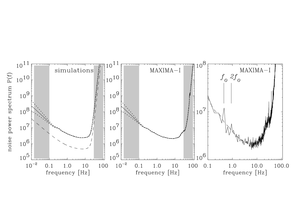
Figure 5: Estimated noise power spectra for simulated and real data. In left panel, the dashed line shows an effective noise power spectrum with $2\beta=1.0$ used for a simulation (its amplitude is scaled down by a factor of 5 to avoid overlapping with solid line). Solid and dotted lines show noise power spectra recovered from this simulation using a prewhitening filter as given by Eq. (7) with $2\beta=1.0$ - solid line; $2\beta=1.25$ (top) and $2\beta=0.75$ (bottom) dotted lines. Middle panel shows noise power spectra for a single segment of the actual maxima-i data. Again the recovery has been made using various prewhitening filters as in the left panel. In all the results displayed in these panels aggressive smoothing have been applied to facilitate better comparison. For actual calculations, such an approach does not have to be the best option. Right panel shows a noise spectrum obtained just as a result of averaging at the second step of the noise estimation procedure, prior to any smoothing. Two small spikes at $\sim 0.45$Hz and $0.9$Hz correspond to a primary mirror chop frequency and its first harmonic. The overplotted dash line is a smoothed version of this spectrum as shown in the middle panel with a solid line. Shaded areas in both left and middle panels show a region of frequencies we marginalize over to avoid either spurious high frequency noise or a noise estimation uncertainty at the low frequency end.

In the following we set the initial width of all the gaps to be no less than twice the effective width of the instrumental filters (which we conservatively choose to be 100 time samples, see Fig. 4), reflecting our ignorance about the origin of some of the gaps. Similarly, we always widen gaps on both sides by an effective filter width when (de)convolving any filter from the raw time stream.

The noise estimation algorithm described here is applied to each time stream segment separately and consists of the following steps:

1. Reducing the noise correlation length, $\lambda_{c}$:
   The time stream segment is convolved with a prewhitening filter,

   $${\hbox{\boldmath$\tilde{d}_{FW}$\unboldmath}}\left(f\right)\equiv\widetilde{W}\left(f\right){\hbox{\boldmath$\tilde{d_{F}}$\unboldmath}}\left(f\right),$$ (6)

   and simultaneously the gaps are widened to account for the width of this filter. The prewhitening filter ($\widetilde{W}$) is usually a half-differencing real filter Tegmark1997design :

   $$\widetilde{W}\left(f\right)\equiv\sin^{\beta}\left(\phi/2\right),$$ (7)

   with a phase $\phi=\pi f\Delta$ and a sampling interval $\Delta$. The prewhitening index, $\beta$, reflects the expected low frequency behavior of a noise power spectrum, i.e., $P\left(f\right)\sim f^{-2\beta}$ for $f\rightarrow 0$. It is adjusted for each segment separately (Fig. 4), so that the prewhitened power spectrum, $P_{W}\left(f\right)\sim\mbox{{\sc const}}$ for $f\rightarrow 0$. The functional form of the prewhitening filter is tested in the subsequent stages of the data analysis, and, if necessary, it may be refined and the entire procedure repeated.

2. Estimating the noise power spectrum of the prewhitened time stream, $P_{FW}\left(f\right)$:
   Sections of the time stream segment are located that have no gaps, are longer than the expected noise correlation length, and are separated from each other by at least this distance. These are used to compute a series of statistically independent estimates of the noise power spectra using standard FFT-based methods (e.g., Press1992 ). These estimates are then checked for stationarity and, if consistent with one another, averaged. If they do not exhibit stationarity then the original time stream segments have to be redefined and made appropriately shorter. The final – average – power spectrum of the stationary noise in a segment can be additionally smoothed and extra(inter)polated to the frequencies corresponding to the full segment.

3. Restoring time stream continuity:
   The gaps are filled with a constrained realization of the noise Hoffman1991 which is assumed to be Gaussian with a power spectrum, $P_{FW}\left(f\right)$, as determined on the previous step and corresponding noise correlation matrix (see Eq. 10), denoted as $N_{t}$ below. The noise within each gap is constrained only by good data samples in its vicinity, i.e., those which are within the noise correlation length, $\lambda_{c}$, of the gap edges,

   $${\hbox{\boldmath$d_{FW}$\unboldmath}}\left(i\right)={\hbox{\boldmath$\xi$\unboldmath}}\left(i\right)+$$ (8)

   $$+\sum_{m,n}{\hbox{\boldmath$N_{t}$\unboldmath}}\left(i,m\right){\hbox{\boldmath$N^{\prime}_{t}$\unboldmath}}^{-1}\left(m,n\right)\left({\hbox{\boldmath$d_{FW}$\unboldmath}}\left(m\right)-{\hbox{\boldmath$\xi$\unboldmath}}\left(m\right)\right).$$

   Here, $N^{\prime}_{t}$ is a $2\lambda_{c}\times 2\lambda_{c}$ matrix describing noise correlations between the time samples just outside of a given gap, $\xi$ is a vector of Gaussian, correlated (but unconstrained) random variables, and $i$ indexes the time samples within a gap. The sum is over $m$ and $n$, both of which index the time samples outside of a given gap which are being used to constrain the noise realization within the gap. Due to required inversion of the matrix $N^{\prime}_{t}$ the computational cost of the procedure is ${\cal O}\left(\lambda_{c}^{3}\right)$ per gap, and it is therefore crucial that $\lambda_{c}$ is sufficiently short.

4. Re-estimating the noise power spectrum:
   The entire time stream segment, with gaps filled, is now used to re-estimate the noise power spectrum. At this stage the low frequency behavior of the noise can be tested; if it is found to be significantly non-flat (i.e., non-white), or to differ from the spectrum estimated at stage 2, then the prewhitening filters used at the stage 1 must be adjusted and the entire sequence repeated.

5. Deconvolving the filters:
   Once the noise power spectrum has been estimated, and the gaps filled with the constrained noise realization, the instrumental and prewhitening filters can be deconvolved from both the time stream and the noise power spectrum. In general, this applies to both the instrumental (or $|\widetilde{X}_{re}\left(f\right)|$) and prewhitening filters. As mentioned above, the deconvolution of the instrumental filters is not always advisable since it may introduce numerical errors. The deconvolution of the prewhitening filter is also sometimes postponed, and accounted for only in the algebra of the map-making algorithm  Tegmark1997design . Such an approach attempts to make use of the shortened correlation length of the prewhitened noise to cut the number of floating point operations required to make the map. In practice we find that it is difficult to take advantage of this in any realistic map-making algorithm (see Sect. III), while, as we argue below, performing the deconvolution at the outset of the noise estimation procedure helps to alleviate a number of problems.

This procedure attempts to estimate the ensemble average noise power spectrum using just one realization of the time stream segment. This is clearly not enough, especially in the presence of correlations on time scales comparable with the length of the segment. Prewhitening helps to alleviate this problem, yet it requires some extra knowledge about the functional form of the prewhitening filter. In this approach, an educated guess, followed by iterative refinement, is then tested a posteriori. For a prewhitening filter of the form given in Eq. (7), we usually find that the power-law index $\beta$ can be uniquely determined with an error not bigger than $|\Delta\beta|\lower 2.15277pt\hbox{$\;\buildrel<\over{\sim}\;$}0.1$ by comparing the power spectra computed at the 2nd and 4th stages of the procedure (see Fig. 5).

Computing and averaging the noise power spectra of the independent, gap-free, sections of a segment (step 2 above) helps to recover a better ensemble average spectrum at intermediate and high frequencies. Smoothing in the frequency domain can also be applied to get even closer to the ensemble average. However, in both cases we need to assume that the real noise power spectrum does not display any significant variation on scales smaller than the smoothing or frequency re-sampling scale.

The result of this procedure is an estimate of the ensemble average noise power spectrum in the time domain which is reliable at sufficiently high frequencies (for maxima-i for $f\lower 2.15277pt\hbox{$\;\buildrel>\over{\sim}\;$}0.1$Hz), but sample-error dominated at the low frequency end ($f\lower 2.15277pt\hbox{$\;\buildrel<\over{\sim}\;$}0.1$Hz). To minimize the effect of the low frequency uncertainty, in the subsequent analysis we marginalize over the low frequency part of the spectrum (see Sect. IV.2).

The entire procedure restores the continuity of the time stream segments: the noise is stationary over an entire segment, including gaps, and the sky signal in gaps is zero. This is important in the subsequent stages of the data analysis; we might worry that adding a random (albeit constrained) signal to the data introduces an extra degree freedom and undermines the uniqness of the result. Although this is true, while different realizations of the random component may indeed lead to slightly different results, all of these results are necessarily statistically equivalent, with no bias introduced. Moreover, the impact of the extra randomness is significantly reduced by the gap pixel marginalization described in Sects. IV.1 &  IV.2. Consequently, we find that, for maxima-i  the final maps and their power spectra are robust and not affected by the random element of this procedure.

Generating constrained noise realizations to fill the gaps is the most time consuming part of this procedure. How important this is for the consistency and accuracy of the entire data analysis pipeline depends on the frequency, size, and regularity of the gaps in a time stream segment. In the case of a handful of narrow, randomly scattered, gaps, an unconstrained, uncorrelated, random noise realization with an rms determined from the rest of the time stream may serve as a convenient first approximation for the analysis.

II.3.2 A time stream with non-negligible sky signal

If the sky signal present in the time stream data is not negligible, but still sub-dominant, then the noise estimation has to be performed iteratively, following an algorithm proposed by Ferreira & Jaffe Ferreira2000 . In this case we distinguish between the full (noise + signal) time stream and the noise-only time stream, where the latter is the noise in the time stream data. At each step of the iteration, a maximum-likelihood map estimated on the previous step is subtracted from the time stream giving the current best estimate of the noise stream (see Sect. V). The above noise power spectrum procedure is applied in full only to the noise time stream; only the instrumental filters deconvolution and related gap-widening are performed on the actual time stream (see Fig. 3). Once the noise estimation has been accomplished, only the noise stream continuity is restored. Therefore the gap time samples from the noise time stream data are used to replace their analogues in the full (unprocessed) time stream. This avoids unnecessarily wasting or biasing good data samples which happen to be in a vicinity of a gap.

A simple extension of this iterative approach also allows us to account for problems related to presence of synchronous systematic signals in the data. We discuss the appropriate algorithms and related issues in some detail in Sect. V.

II.4 The time domain noise correlation matrix

Formally, maximum likelihood map-making requires the full time-time noise correlation matrix, rather than just a noise power spectrum. For an idealized time stream the former is just the Fourier transform of the latter,

$${\hbox{\boldmath$N_{Ct}$\unboldmath}}\left(i,j\right)\equiv\int df\,P\left(f\right)\exp\left(-2\pi\iota f(i-j)\Delta\right).$$ (9)

For a finite time stream this expression leads to a circulant matrix denoted by the subscript $C$ Golub1983 . If the correlation length in the time stream is less than half of the time stream length, then an alternative approximate correlation matrix, $N_{t}$, is given by

$${\hbox{\boldmath$N_{t}$\unboldmath}}\left(i,j\right)\simeq\left\{\begin{array}[]{l l}\displaystyle{{\hbox{\boldmath$N_{Ct}$\unboldmath}}\left(i,j\right);}&\displaystyle{\mbox{if }|i-j|<\lambda_{c},}\\ \displaystyle{0;}&\displaystyle{\mbox{otherwise.}}\end{array}\right.$$ (10)

In practise, numerical error in the estimation (and Fourier transform) of the noise power spectrum means that $N_{t}$ computed in this way may not even be positive definite. Such problems can be alleviated by the introduction of an extra power spectrum smoothing window, $S\left(f\right)$, designed to truncate smoothly the correlations once their amplitude reaches the limits of numerical accuracy. Again, it is prudent to apply the window function prior to deconvolving the prewhitening filter. Eq. (9) then assumes a somewhat more complicated form,

$${\hbox{\boldmath$N_{Ct}$\unboldmath}}\left(i,j\right) = \int df\,|\widetilde{W}\left(f\right)|^{-2}\exp\left(-2\pi\iota f(i-j)\Delta\right)$$ (11)

$$\times \int df^{\prime}\,S\left(|f-f^{\prime}|\right)P_{W}\left(f^{\prime}\right),$$

where $\widetilde{W}\left(f\right)$ is given by Eq. (7). In the following, we make use of this expression whenever computing $N_{Ct}$. Its inverse is approximated by an analogous formula Golub1983 ,

$${\hbox{\boldmath$N_{Ct}$\unboldmath}}^{-1}\left(i,j\right) = \int df\,|\widetilde{W}\left(f\right)|^{2}\exp\left(-2\pi\iota f(i-j)\Delta\right)$$ (12)

$$\times \int df^{\prime}\,S\left(|f-f^{\prime}|\right)P_{W}^{-1}\left(f^{\prime}\right).$$

Our usual choice for $S(f)$ is a Gaussian with an appropriately tuned width (typically of $1000-5000$ time samples for maxima-i).

III Map-making: formalism

III.1 The basic framework

The procedure described above provides the input for the map-making per se; here, we take as given the time stream data with instrumental filters deconvolved and gaps filled, and the corresponding noise power spectrum for each segment.

In this Section we consider a case of a somewhat idealized time stream, leaving a discussion of the fully realistic case to Sect. IV. We consider a time stream consisting of a single segment, neglect most of the systematic contributions, but do admit the presence of (now filled) gaps in the data. The simplified Eq. (1) reads now,

$${\hbox{\boldmath$d_{t}$\unboldmath}}={\hbox{\boldmath$A$\unboldmath}}{\hbox{\boldmath$m_{p}$\unboldmath}}+{\hbox{\boldmath$n_{t}$\unboldmath}}.$$ (13)

Here $A$ is a pointing matrix assigning each time sample to an appropriate pixel (or a set of pixels in a case of differencing experiments) on the sky (as observed at the given time) with the sky signal given by a pixelized map: $m_{p}$. $n_{t}$ is the (Gaussian) noise time stream with correlations given by the power spectrum estimated as in the previous Section.

In this case we can write a closed form solution for the map Wright1996a ; Tegmark1997design (but see ). The maximum likelihood estimates of the map, $m_{p}$, and the pixel-pixel noise correlation matrix, $N_{p}$, then read,

$$m_{p} = \left({\hbox{\boldmath$A^{T}$\unboldmath}}{\hbox{\boldmath$M$\unboldmath}}{\hbox{\boldmath$A$\unboldmath}}\right)^{-1}\,{\hbox{\boldmath$A^{T}$\unboldmath}}{\hbox{\boldmath$M$\unboldmath}}{\hbox{\boldmath$d_{t}$\unboldmath}},$$ (14)

$$N_{p} = \left({\hbox{\boldmath$A^{T}$\unboldmath}}{\hbox{\boldmath$M$\unboldmath}}{\hbox{\boldmath$A$\unboldmath}}\right)^{-1}\left({\hbox{\boldmath$A^{T}$\unboldmath}}{\hbox{\boldmath$M$\unboldmath}}{\hbox{\boldmath$N_{t}$\unboldmath}}{\hbox{\boldmath$M$\unboldmath}}{\hbox{\boldmath$A$\unboldmath}}\right)\left({\hbox{\boldmath$A$\unboldmath}}^{T}{\hbox{\boldmath$M$\unboldmath}}{\hbox{\boldmath$A$\unboldmath}}\right)^{-1}.$$ (15)

Here, $M$ is a positive-definite symmetric matrix, and $N_{t}$ the time domain noise correlation matrix (Eq. 10). If ${\hbox{\boldmath$M$\unboldmath}}={\hbox{\boldmath$N_{t}$\unboldmath}}^{-1}$, then Eqs. (14) & (15) give minimum variance estimates of $m_{p}$ and $N_{p}$. Other choices trade a larger variance for increased computational speed. In particular Tegmark Tegmark1997design proposed the choice for $M$ of the circulant part of the $N_{t}$ matrix. We discuss this option in Sect. III.3 below.

In the following we present some different approaches and their application to a realistic maxima-like data set.

III.2 Minimum variance approaches

III.2.1 Exact methods

With ${\hbox{\boldmath$M$\unboldmath}}={\hbox{\boldmath$N_{t}$\unboldmath}}^{-1}$, we get the minimum variance estimates,

$$m_{p} = \left({\hbox{\boldmath$A^{T}$\unboldmath}}{\hbox{\boldmath$N_{t}$\unboldmath}}^{-1}{\hbox{\boldmath$A$\unboldmath}}\right)^{-1}\,{\hbox{\boldmath$A^{T}$\unboldmath}}{\hbox{\boldmath$N_{t}$\unboldmath}}^{-1}{\hbox{\boldmath$d_{t}$\unboldmath}},$$ (16)

$$N_{p} = \left({\hbox{\boldmath$A^{T}$\unboldmath}}{\hbox{\boldmath$N_{t}$\unboldmath}}^{-1}{\hbox{\boldmath$A$\unboldmath}}\right)^{-1}.$$ (17)

The exact implementation of these equations seems a daunting task. The time stream length may easily reach many tens and hundreds of million of samples, making exact inversion of the time domain noise correlation matrix prohibitive. However, for a maxima-i like experiment with segments lengths reaching only ${\cal O}\left(10^{5}\right)$ samples an exact implementation is feasible on a moderately powerful workstation.

At the core of the implementation lies the observation that for a gap-free time stream of the length $n_{s}$ with stationary noise the time domain noise correlation matrix is Toeplitz, with ${\hbox{\boldmath$N_{t}$\unboldmath}}\left(i,j\right)={\hbox{\boldmath$N_{t}$\unboldmath}}\left(\left|i-j\right|,0\right)$. The inversion of a Toeplitz matrix can be performed in as few as ${\cal O}\left(n_{s}^{2}\right)$ operations – clearly feasible for ${\cal O}\left(10^{5}\right)$ time samples – and even faster algorithms are possible (e.g., Golub1983 ) bringing that number down to ${\cal O}\left(n_{s}\log^{2}n_{s}\right)$. The number of operations can be further reduced if the noise correlation length is shorter than the time stream segment length and the noise correlation matrix is therefore band-diagonal.

If gaps are present in the time stream then, in principle, the Toeplitz (stationary) character of the time domain noise correlation matrix is lost. However the gap-filling procedure described above is explicitly designed to restore the stationarity of the noise in the time stream. Since the gap samples contain no sky signal (by construction) they can be treated as data taken while observing a fictitious signal-free pixel in the sky map $m_{p}$. Once the map and its noise matrix are estimated, this extra gap pixel is rejected from the map and the pixel domain noise correlation matrix (effectively marginalizing over it). This is a special application of the extra pixel method discussed in detail below (see Sect. IV.1 and also  daCosta1999 ).

The computational effort then scales with a number of pixels $n_{pix}$ and a number of time samples $n_{s}$ as:

• noise inverse in time domain:
                        ${\hbox{\boldmath$N_{t}$\unboldmath}}\longrightarrow{\hbox{\boldmath$N_{t}$\unboldmath}}^{-1}$ : ${\cal O}\left(n_{s}^{2}\right)$;

• noise inverse in pixel domain:
                        ${\hbox{\boldmath$N_{t}$\unboldmath}}^{-1},{\hbox{\boldmath$A$\unboldmath}}\longrightarrow{\hbox{\boldmath$A$\unboldmath}}^{T}{\hbox{\boldmath$N_{t}$\unboldmath}}^{-1}{\hbox{\boldmath$A$\unboldmath}}$ : ${\cal O}\left(n_{s}^{2}\right)$;

• noise weighted map:
                        ${\hbox{\boldmath$N_{t}$\unboldmath}}^{-1},{\hbox{\boldmath$A$\unboldmath}},{\hbox{\boldmath$d_{t}$\unboldmath}}\longrightarrow{\hbox{\boldmath$A$\unboldmath}}^{T}{\hbox{\boldmath$N_{t}$\unboldmath}}^{-1}{\hbox{\boldmath$d_{t}$\unboldmath}}$ : ${\cal O}\left(n_{s}^{2}\right)$;

• noise matrix in pixel domain:
                        ${\hbox{\boldmath$N_{p}$\unboldmath}}^{-1}\longrightarrow{\hbox{\boldmath$N_{p}$\unboldmath}}$ : ${\cal O}\left(n_{pix}^{3}\right)$;

• final map:
                        ${\hbox{\boldmath$N_{p}$\unboldmath}},{\hbox{\boldmath$A$\unboldmath}}^{T}{\hbox{\boldmath$N_{t}$\unboldmath}}^{-1}{\hbox{\boldmath$d_{t}$\unboldmath}}\longrightarrow{\hbox{\boldmath$N_{p}$\unboldmath}}\left({\hbox{\boldmath$A$\unboldmath}}^{T}{\hbox{\boldmath$N_{t}$\unboldmath}}^{-1}{\hbox{\boldmath$d_{t}$\unboldmath}}\right)$ : ${\cal O}\left(n_{pix}^{2}\right)$.

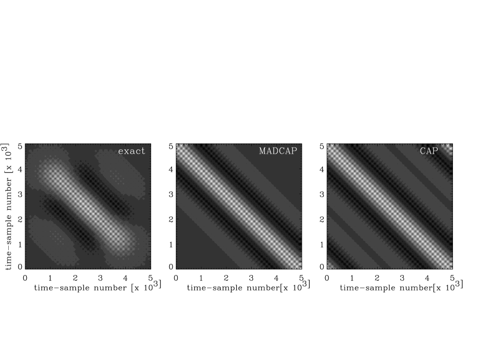
Figure 6: Inverse time-domain noise correlation matrices computed using MADCAP (middle panel) and circulant (right) approximations and compared with the exact result (left). For visualization purposes the time-stream segment length assumed here is only $5,000$ samples and the correlation length, $\lambda_{c}\simeq 1000$.

For the first three items substantial savings can be made if the inverse time-time noise correlation matrix, ${\hbox{\boldmath$N_{t}$\unboldmath}}^{-1}$, is assumed to be band-diagonal – an approximation usually well fulfilled for the inverse of a band-diagonal noise correlation matrix. If this is the case, and, in addition, the time domain correlation length is short, then the inverse pixel-pixel noise correlation matrix, ${\hbox{\boldmath$N_{p}$\unboldmath}}^{-1}$, is often rather sparse. In this case additional savings can be made by using the sparse matrix algorithms, e.g., Sherman-Morrison-Woodbury formula (e.g., Press1992 ) to calculate both the map and the noise correlation matrix in the pixel domain.

The memory requirements are also reduced by considering the various matrices’ structure. Since we only need to keep the first row of the Toeplitz $N_{t}$ matrix and we do not need ${\hbox{\boldmath$N_{t}$\unboldmath}}^{-1}$ explicitly, the major memory requirements are set by the size of the ${\hbox{\boldmath$A$\unboldmath}}^{T}{\hbox{\boldmath$N_{t}$\unboldmath}}^{-1}$ matrix, which is ${\cal O}\left(n_{pix}n_{s}\right)$, and of the noise correlation for the map, ${\cal O}\left(n_{pix}^{2}\right)$. Note that the first of these limits can be reduced at the expense of the operation counts, since there is no need to save all $n_{pix}n_{s}$ elements of this matrix provided we are prepared to re-calculate them as needed.

III.2.2 Approximate methods

One way to speed up map-making, while at the same time providing a good approximation to the optimal minimum variance map was proposed by Ferreira and Jaffe Ferreira2000 and incorporated into the MADCAP package by Borrill Borrill1999mad . Rather than explicitly inverting the $N_{t}$ matrix we instead use the approximation,

$${\hbox{\boldmath$N_{t}$\unboldmath}}^{-1}\left(i,j\right)\simeq\left\{\begin{array}[]{cl}{\hbox{\boldmath$N_{Ct}$\unboldmath}}^{-1}\left(i,j\right),&\mbox{\rm if }|i-j|\leq\min\left(n_{s}/2,\lambda_{c}\right),\\ 0,&\mbox{\rm else.}\\ \end{array}\right.$$ (18)

Here $n_{s}$ and $\lambda_{c}$ are the time stream and correlation lengths respectively, and the subscript $C$ denotes the circulant part of the noise correlation matrix (Eq. 11). Apart from this approximation, the remaining steps follow precisely as before. Hereafter we refer to this approach as the MADCAP approximation.

Inversion of a circulant matrix can be accomplished using FFTs (Eq. 12) in only ${\cal O}\left(n_{s}\log n_{s}\right)$ operations. This approach is therefore designed to reap the benefits of Fast Fourier methods, while at the same time providing a good approximation to the exact solution. If $n_{s}\gg 4\lambda_{c}$ the fraction of ${\hbox{\boldmath$N_{t}$\unboldmath}}^{-1}$ matrix elements seriously misestimated (i.e., affected by the segment ‘edge’ effects, see Fig. 6) by this procedure should only be ${\cal O}\left(4\lambda_{c}^{2}/n_{s}^{2}\right)$, and its performance in the large $n_{s}$ limit should be satisfactory. However, because the inverse of a Toeplitz matrix is Teoplitz only when it is also circulant this is the only case when this approach is exact. We demonstrate how well this approximation fares in reproducing the pixel domain map and noise correlation matrix in realistic cases below (Sect. III.4).

The operation count changes only for the two items in the list, which now read,

• noise inverse in time domain:
                        ${\hbox{\boldmath$N_{t}$\unboldmath}}\longrightarrow{\hbox{\boldmath$N_{t}$\unboldmath}}^{-1}$ : ${\cal O}\left(n_{s}\log n_{s}\right)$;

• noise weighted map:
                        ${\hbox{\boldmath$N_{t}$\unboldmath}}^{-1},{\hbox{\boldmath$A$\unboldmath}},{\hbox{\boldmath$d_{t}$\unboldmath}}\longrightarrow{\hbox{\boldmath$A$\unboldmath}}^{T}{\hbox{\boldmath$N_{t}$\unboldmath}}^{-1}{\hbox{\boldmath$d_{t}$\unboldmath}}$ : ${\cal O}\left(n_{s}\log n_{s}\right)$.

The scaling of the noise weighted map operation count above assumes the use of FFTs for the Toeplitz matrix multiplication – a trick explained in Golub1983 . The memory requirement is set either by the larger of the size of the noise matrix in the pixel domain $n_{pix}^{2}$ or the time stream length $n_{s}$. If an efficient, fast – ${\cal O}\left(n_{s}\log^{2}n_{s}\right)$ – implementation of the Toeplitz matrix inversion is viable then, at least in the common case of an approximately band-diagonal inverse noise correlation matrix ${\hbox{\boldmath$N_{t}$\unboldmath}}^{-1}$, the major computational advantage of the approximate method over the exact one would vanish, and the memory requirement would remain as its only asset.

III.3 Circulant approaches

If we take ${\hbox{\boldmath$M$\unboldmath}}={\hbox{\boldmath$N_{Ct}$\unboldmath}}^{-1}$ then the noise correlation matrix in the pixel domain can be expressed as Tegmark1997design ,

$$N_{p} = {\hbox{\boldmath$N_{Cp}$\unboldmath}}+{\hbox{\boldmath$N_{Sp}$\unboldmath}},$$

$$N_{Cp} \equiv \left({\hbox{\boldmath$A$\unboldmath}}^{T}{\hbox{\boldmath$N_{Ct}$\unboldmath}}^{-1}{\hbox{\boldmath$A$\unboldmath}}\right)^{-1},$$ (19)

$$N_{Sp} \equiv {\hbox{\boldmath$N_{Cp}$\unboldmath}}\left({\hbox{\boldmath$A$\unboldmath}}^{T}{\hbox{\boldmath$N_{Ct}$\unboldmath}}^{-1}{\hbox{\boldmath$N_{St}$\unboldmath}}{\hbox{\boldmath$N_{Ct}$\unboldmath}}^{-1}{\hbox{\boldmath$A$\unboldmath}}\right){\hbox{\boldmath$N_{Cp}$\unboldmath}},$$

where the time domain noise correlation matrix has been decomposed into its circulant ($N_{Ct}$) and sparse ($N_{St}$) parts,

$${\hbox{\boldmath$N_{t}$\unboldmath}}\equiv{\hbox{\boldmath$N_{Ct}$\unboldmath}}+{\hbox{\boldmath$N_{St}$\unboldmath}}.$$ (20)

The sparse term compensates for the off-diagonal corners of the circulant matrix. As in the case of the MADCAP approximation, the only inversion required in the time domain is that of a circulant matrix. Hence it has been argued that, because the $N_{St}$ matrix should be very sparse, the operation count in this approach should be significantly lower than in the exact minimum variance approach Tegmark1997design .

The disadvantage of this approach is not in the non-minimum-variance map that results (since the loss of precision is usually insignificant) but rather in implementing its more complicated algebra. If no assumption is made about band-diagonality, then the computational costs scale as:

• noise inverse in time domain:
  ${\hbox{\boldmath$N_{Ct}$\unboldmath}}\longrightarrow{\hbox{\boldmath$N_{Ct}$\unboldmath}}^{-1}$ : ${\cal O}\left(n_{s}\log n_{s}\right)$;

• noise inverse in pixel domain:
  circulant part:
  ${\hbox{\boldmath$N_{Ct}$\unboldmath}}^{-1},{\hbox{\boldmath$A$\unboldmath}}\longrightarrow{\hbox{\boldmath$A$\unboldmath}}^{T}{\hbox{\boldmath$N_{Ct}$\unboldmath}}^{-1}{\hbox{\boldmath$A$\unboldmath}}$ : ${\cal O}\left(n_{s}^{2}\right)$;
  sparse part:
  ${\hbox{\boldmath$N_{St}$\unboldmath}},{\hbox{\boldmath$N_{Ct}$\unboldmath}}^{-1},{\hbox{\boldmath$A$\unboldmath}}\longrightarrow$
           ${\hbox{\boldmath$A$\unboldmath}}^{T}{\hbox{\boldmath$N_{Ct}$\unboldmath}}^{-1}{\hbox{\boldmath$N_{St}$\unboldmath}}{\hbox{\boldmath$N_{Ct}$\unboldmath}}^{-1}{\hbox{\boldmath$A$\unboldmath}}$ : ${\cal O}\left(n_{pix}n_{s}^{2}\right)$;

• noise weighted map:
  ${\hbox{\boldmath$N_{Ct}$\unboldmath}}^{-1},{\hbox{\boldmath$A$\unboldmath}},{\hbox{\boldmath$d_{t}$\unboldmath}}\longrightarrow{\hbox{\boldmath$A$\unboldmath}}^{T}{\hbox{\boldmath$N_{Ct}$\unboldmath}}^{-1}{\hbox{\boldmath$d_{t}$\unboldmath}}$ : ${\cal O}\left(n_{s}\log n_{s}\right)$;

• noise matrix in pixel domain:
  ${\hbox{\boldmath$N_{p}$\unboldmath}}^{-1}\longrightarrow{\hbox{\boldmath$N_{p}$\unboldmath}}$ : ${\cal O}\left(n_{pix}^{3}\right)$.

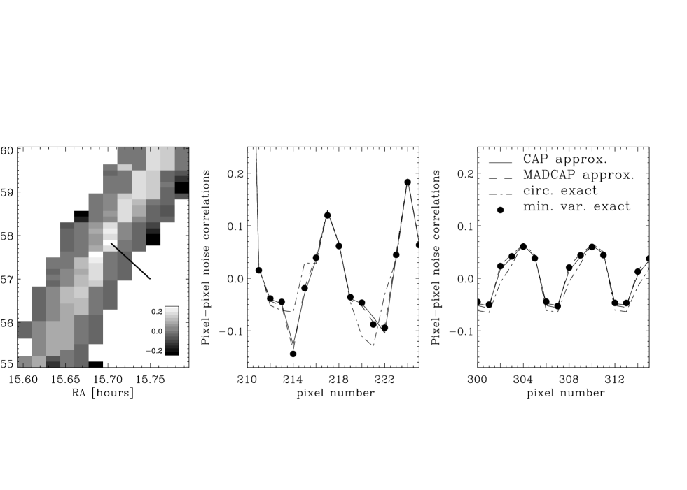
Figure 7: An example of pixel domain noise correlations estimated for a single segment of maxima-i data set. In this figure, we show correlations of a single selected pixel with its neighbors. This pixel is marked in left panel with an arrow. The color scale shows the correlation level relative to the RMS value of the noise in the selected pixel. The scanning direction was from the left bottom corner to the top right, leaving a smudge of strong correlations in pixel domain. Pixels are numbered row by row from the left to the right and from the bottom to the top as shown in the left panel. Note a strongly distorted aspect ratio of the figure due to a scan elongation in a declination direction. These correlations as a function of a pixel number are also displayed in the middle and right panels. They show the relative correlations of the selected pixel with its closer (middle) and more distant neighbors (right panel). The chosen pixel has a number 210. Different lines correspond to different map-making methods used for the correlation estimations. Filled circles show results of the exact minimum variance, solid line - approximate circulant (CAP), dashed - approximate MADCAP and dot-dashed - exact circulant methods.

Note that the operation count is dominated by the sparse inverse computation ($n_{s}>n_{pix}$). The operation count can be reduced if $N_{t}$ and $N_{Ct}$ are assumed to be band diagonal. However, even then, for experiments like maxima the operation count remains ${\cal O}\left(n_{s}^{2}\right)$, usually with a large prefactor. Hence this approach is far from competitive with those discussed above, although it can be comparable for very short correlation length data. The memory required again scales as ${\cal O}\left(n_{pix}n_{s}\right)$.

A possible approximation, which we advocate hereafter, is to neglect the sparse correction completely in the expression for the pixel-pixel noise correlation matrix. Clearly the operation count drops to ${\cal O}\left(n_{s}^{2}\right)$ or ${\cal O}\left(n_{pix}^{3}\right)$ – whichever is larger – and is usually ${\cal O}\left(n_{pix}^{3}\right)$ especially if ${\hbox{\boldmath$N_{Ct}$\unboldmath}}^{-1}$ is assumed to be band diagonal. In this case the method’s computational requirements are comparable with those of the MADCAP algorithm Borrill1999mad . In the following we refer to this approach as the circulant approximation (CAP). This approximation is clearly very similar to the MADCAP approach discussed above, although it is strictly exact for a diagonal noise correlation matrix as well as for an infinitely long time stream.

III.4 Comparison and assessment

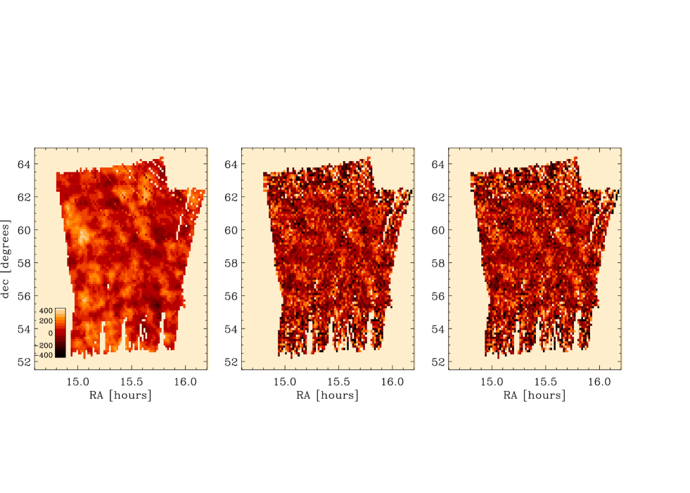
Figure 8: Simulated maxima-i-like maps of the CMB anisotropy. Left panel shows the simulated map used for creating the time stream data of a single detector of a maxima-like experiment. The time stream was subsequently used to recover the map of the sky applying the approximate CAP (middle) and MADCAP algorithms.

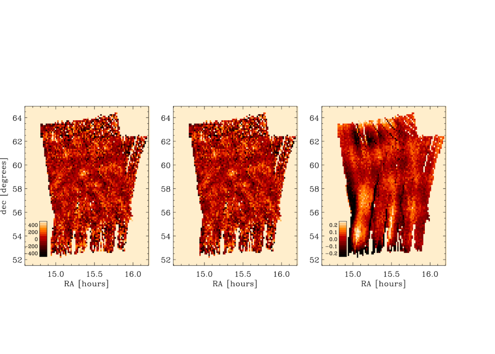
Figure 9: Comparison of two map-making algorithms applied to the real maxima-i data of a single photometer. The left panel shows the map computed using the approximate circulant (CAP) approach. The middle panel shows the map recovered using MADCAP approach. The difference of both divided by an estimated rms of the pixel noise is shown in a right panel. Note that the color stretch limits are from -0.25 to 0.25 in the right panel.

Although the various map-making methods outlined above are algebraically similar, being derived from the same underlying equations, their implementations and generalized extensions to fully realistic time streams differ considerably.

The approximate methods are of particular interest, because they achieve the speed of Fast Fourier transforms. If that is attained without sacrificing the necessary precision is to be tested and may depend on the particular case at hand. The important parameters are the noise correlation length ($\lambda_{c}$) and the time stream length ($n_{s}$). If these numbers are comparable the differences between the methods can be significant, but they should disappear whenever $\lambda_{c}\ll n_{s}$ and ‘edge’ effects are unimportant. Given the presence of a so-called $1/f$ noise component in the time stream, the assumption that $\lambda_{c}$ is independent of the time stream length may seem to be plainly wrong. Instead the correlations should be present on time scales comparable with the time stream length. However, a low frequency cutoff (e.g., AC high passing filter in the maxima experiment) usually limits the correlation length independent of the time stream length.

Here we address and illustrate those issues using the maxima-i experiment as an example. For this experiment the average length of the time stream segments is around $50,000$ samples, with some segments as short as $35,000$ samples. The very gradual decay of the correlations with time makes it difficult to determine the correlation length precisely. However, we have found that the dependence of the resulting map on the value of $\lambda_{c}$ assumed vanishes before $\lambda_{c}$ reaches $10,000$ samples, and have therefore used $\lambda_{c}=10,000$ in all computations. Hence, for maxima-i, $\lambda_{c}$ is less than but not negligible to $n_{s}$, and prior to taking advantage of the speed of the approximate methods we need to demonstrate their applicability.

Note that comparing the different methods is not entirely straightforward. Assumptions about the band-diagonality of either the time domain noise correlation matrix or its inverse, as required by the different methods, are clearly not equivalent. The relation between the assumed bandwidths of these matrices is also not obvious. It may seem that a fair comparison would be to take the bandwidths to be as large as possible in all methods. However, we then run into the problem of numerical inaccuracies unavoidably present in the calculation of the noise correlation matrix (or its inverse), especially at large time lags, which can result in a non-positive definite (unphysical) noise correlation matrix in pixel domain. Although power spectrum windowing (see Eqs. 11, 12) can be used to alleviate numerical problems of this sort, this may also have different consequences for each of the methods.

This point is particularly conspicuous when comparisons are made with the exact circulant method. We find that this approach is very sensitive to both the choice of $\lambda_{c}$ and the windowing technique. For this reason we do not quote precise numbers for the comparison of this method with the others. By adjusting the free parameters of the method we can reproduce other methods’ results quite accurately, and within the expected statistical uncertainty of the maps.

In the case of the other comparisons we have applied a Gaussian window function (Eqs. 11, 12) while computing the noise power spectrum and kept similar correlation lengths for all three methods. In any case, the numbers quoted below should be looked at as indicative rather than as the best case possible.

We choose to compare maps and noise correlation matrices directly in pixel domain, notwithstanding the fact that the approximations are really applied when the inverse of the noise correlation matrix in the time domain is computed (see Fig. 6). It is the quality of the estimate of the map and its noise correlation matrix which matter for any subsequent analysis. Such an approach also seems to be more general than assessing the quality of a map through the application of a specific statistical tool.

A sample of results is shown in Fig. 7. The middle and right panels show two regimes of pixel-domain noise correlations as estimated using different methods. The left panel shows the correlations of a selected pixel with all the others as projected on the sky. These were computed for a single $\sim 40,000$-sample segment of the CMB1 scan covering an area of $\sim 6$ square degrees on the sky, corresponding to $\sim 400$ square 8arcm pixels. Neither filtering nor marginalization has been applied to the time ordered data. The agreement between results from the different methods is generally quite good. More quantitatively, $\sim 98$% of the matrix elements show relative differences less than $20$% when computed using the exact minimum variance approach and the MADCAP approximation, and $\sim 50$% show differences less than $5$%. Similar numbers are found for the comparison of this exact method and the CAP approximation. Usually, both approximate methods tend to overestimate high positive correlations. The MADCAP approach also seems to underestimate the amplitude of negative correlations, yet frequently recovers weak correlations more precisely than the other approximation. The relative differences of the maps are of the order of $10$% (Fig. 8), which, on average, amounts to no more than $10$% of the rms noise level predicted for a given pixel (Fig. 9).

To test if the discrepancies are due to numerical errors, rather than differences in the algorithms, we use the exact method with an explicitly circulant noise correlation matrix, and compare the result with that calculated using the approximate circulant approach. In the absence of numerical inaccuracies both results should be identical. We find that the differences are predominantly at the $2-3$% level. We obtain similar error estimates when analyzing a diagonal noise correlation matrix using all three methods.

We can also ask if there is any systematic error incurred as a consequence of the approximations which bias the results of a particular approach. One way to address this issue with simulated maps is to check whether the actual noise in an estimated map is properly described by a concurrently estimated noise correlation matrix. This is clearly the case for the exact methods, which are derived to obey such a requirement. To test the approximate approaches we define $m_{sky}$ as the true noiseless map of the sky used for a simulation. $m_{c}$, $N_{c}$, and $m_{m}$, $N_{m}$ are maps and pixel-pixel noise correlation matrices as estimated by the CAP and MADCAP approximate methods respectively. For each of the noise matrices we introduce a matrix ${\hbox{\boldmath$N_{i}$\unboldmath}}^{-1/2}$ such that ${\hbox{\boldmath$N_{i}$\unboldmath}}^{-1/2}\left({\hbox{\boldmath$N_{i}$\unboldmath}}^{-1/2}\right)^{T}={\hbox{\boldmath$N_{i}$\unboldmath}}^{-1}$. Consequently the variable $y_{i}$, defined as

$${\hbox{\boldmath$y_{i}$\unboldmath}}\equiv{\hbox{\boldmath$N_{i}$\unboldmath}}^{-1/2}\left({\hbox{\boldmath$m_{i}$\unboldmath}}-{\hbox{\boldmath$m_{sky}$\unboldmath}}\right),\ \ \ {\hbox{\boldmath$i=c,m$\unboldmath}},$$ (21)

should be a vector of uncorrelated, Gaussian variables with a dispersion equal to unity if no systematic problem is introduced by an approximation. This can be tested using, e.g., the Kolmogorov-Smirnov test (see also Sect. VI). Such a test is comfortably passed by both methods for noise in the pixel domain ranging from $\sim 100\mu$K per 8 arcminute pixel (the maxima-i single channel level) down to $\sim 60\mu$K (the maxima-i 4-channel combined level).

The differences between the results of the various methods, as summarized above, are found to be rather small, and indicate that all the methods may be equivalent in practice. Although the problem is difficult to tackle in a more quantitative and general way, it can be addressed from the point of view of specific statistics derived from the maps. An example of such a test, comparing the power spectrum statistic, is shown in Fig. 10. In this case the power spectra of the maxima-i maps computed using both map-making methods show very good agreement.

Figure 10: Comparison of power spectra computed for the maps made with two different map-making algorithms as shown in two left panels of Fig. 9. The data are those of a single maxima-i detector. Circles show the results for the map made using approximate circulant (CAP) algorithm, and diamonds show the results for the map made using the MADCAP approximation.

In practise, the approximate methods have an advantage over the exact methods of being easily implementable. In fact, both can be straightforwardly applied using the MADCAP package Madcap . The differences in the results provide some insight into the sensitivity of the results to the treatment of time domain noise correlations. More to the point, the result of any statistical test applied to the map, which depends on the choice of the approximate method used during map-making, should be treated with suspicion. We have demonstrated that for the maxima-i data analysis and, in particular, for power spectrum estimation, the differences between the methods are negligible.

In summary, all four map-making methods are broadly consistent at the noise level of the maxima-i maps. This concordance is only expected to improve if longer time stream segments are considered. Numerical errors can readily be kept under control even with as many as ${\cal O}\left(10^{5}-10^{6}\right)$ time samples, at least for maxima-like data sets, although further tests may be needed for low noise cases. Both approximate methods are easy to implement, with their speed being limited by the pixel domain noise correlation matrix inversion. The exact minimum variance method provides a useful cross-check on both the validity of the approximations and numerical error propagation, and, with further improvements may be able to achieve the computational speed of the approximate approaches.

We note again that all of this assumes a continuous time stream with stationary noise resulting from application of the gap filling algorithm; the restoration of the Toeplitz character of the noise correlations is crucial for the feasibility of the exact minimum variance approach, as well for as the accuracy of the approximate methods.

IV Map-making: amendments

So far we have been assuming an ‘optimistic’ model for the signal in the time stream, $d_{t}$ (Eq. 13). Commonly, unwanted contributions (e.g., the overall average temperature, primary mirror- or gondola- synchronous noise) are present in the data (Eq. 1) and have to be dealt with if a reliable result is to be obtained.

Let us consider a case of an arbitrary time domain contribution of known temporal behavior. We take these to be given by a set of $m$ template vectors $\tau_{t}^{\left(i\right)}$, of unknown amplitudes, $x^{\left(i\right)}$, so the resulting time stream equation is

$${\hbox{\boldmath$d_{t}$\unboldmath}}={\hbox{\boldmath$A$\unboldmath}}{\hbox{\boldmath$m_{p}$\unboldmath}}+{\hbox{\boldmath$n_{t}$\unboldmath}}+\sum_{i=1}^{m}x^{\left(i\right)}{\hbox{\boldmath$\tau_{t}^{\left(i\right)}$\unboldmath}}.$$ (22)

The additional number $x^{\left(i\right)}$ can be formally treated as an extra (fictitious) pixel ‘observed’ with a ‘pointing matrix’ as given by $\tau_{t}^{\left(i\right)}$. These additional numbers can be estimated during the course of a map-making procedure and then marginalized over. Alternatively, the entire extra term, $\sum_{i}x^{\left(i\right)}{\hbox{\boldmath$\tau_{t}^{\left(i\right)}$\unboldmath}}$, can be thought of as a part of the noise term and directly marginalized over in the course of map-making. Clearly these two approaches are just different implementations of the same idea, yet, depending on the particular problem at hand, one or the other may be more appropriate. In the following, we refer to them as the extra pixels and marginalization methods, respectively, and discuss them and some of their applications.

IV.1 Extra pixels.

Let us define a vector $x_{q}$ as,

$${\hbox{\boldmath$x_{q}$\unboldmath}}^{T}\equiv\left[x^{\left(1\right)},\cdots,x^{\left(m\right)}\right],$$ (23)

and a matrix $B$ such that,

$${\hbox{\boldmath$B$\unboldmath}}\equiv\left[{\hbox{\boldmath$\tau_{t}^{\left(1\right)}$\unboldmath}},\cdots,{\hbox{\boldmath$\tau_{t}^{\left(m\right)}$\unboldmath}}\right].$$ (24)

We can now rewrite Eq. (22) as,

$${\hbox{\boldmath$d_{t}$\unboldmath}}={\hbox{\boldmath$A$\unboldmath}}{\hbox{\boldmath$m_{p}$\unboldmath}}+{\hbox{\boldmath$B$\unboldmath}}{\hbox{\boldmath$x_{q}$\unboldmath}}+{\hbox{\boldmath$n_{t}$\unboldmath}}.$$ (25)

From this it is clear that the extra time stream contribution can be thought of as a set of extra (fictitious) pixels ($x_{q}$) ‘observed’ with a pointing matrix given by $B$. If we, furthermore, recast this equation as,

$${\hbox{\boldmath$d_{t}$\unboldmath}}=\left[{\hbox{\boldmath$A$\unboldmath}},{\hbox{\boldmath$B$\unboldmath}}\right]\left[\begin{array}[]{c}{\hbox{\boldmath$m_{p}$\unboldmath}}\\ {\hbox{\boldmath$x_{q}$\unboldmath}}\end{array}\right]+{\hbox{\boldmath$n_{t}$\unboldmath}}\equiv{{\cal A}}{{\hbox{\boldmath$\hat{m}_{p}$\unboldmath}}}+{\hbox{\boldmath$n_{t}$\unboldmath}},$$ (26)

we find that it is formally identical to Eq. (13). Here, we have introduced a generalized pointing matrix, ${\cal A},$ and a generalized map, $\hat{m}_{p}$. Those correspond to an ‘ordinary’ map and a pointing matrix, but now extended to incorporate also the extra pixels. The map-making methods discussed above can all be applied in the present case, with all their caveats and strengths. The appropriate equations preserve the form of Eqs. (14) & ( 15) but the pointing matrix, $A$, the map, $m_{p}$, and the pixel domain noise correlation matrix, $N_{p}$, need to be replaced by their generalized counterparts, i.e., ${\cal A},$ $\hat{m}_{p}$ and ${\cal N}_{p}$ respectively. As a result, the map-making procedure provides an estimate of a generalized map and a generalized noise correlation matrix in pixel domain.

In addition to the minimum-variance considerations described above, the formalism so far described can also be thought of as describing the likelihood function for the data: the distribution of the underlying (generalized) map is Gaussian with mean and variance as given by Eqs. (16) & (17) (or approximations to these). Thus, the generalized map is a simultaneous estimate of both the real map and the ‘extra’ pixels. Knowledge of the amplitudes of these extra pixels are often useful for diagnostic purposes. However, we are in the end interested in the real map itself; hence we wish to marginalize over the $x_{q}$. With a uniform prior, we find the usual Gaussian results:

• the marginalized map is just the generalized map with the extra pixels removed; and

• the marginalized noise matrix is just the generalized noise matrix with the rows and columns corresponding to the extra pixels removed.

Clearly, only well-understood features of the time stream, for which the pointing operator $B$ is known, can be accounted for using this approach. Moreover, if the extra component is indistinguishable from the CMB temperature map, i.e., is sky-stationary, then the clean separation of the map into CMB and non-CMB components is impossible. That is manifested as a singularity of the ${\cal A}^{T}{\hbox{\boldmath$M$\unboldmath}}{\cal A}$ (see Eqs. 14 & 15) matrix. In some cases, if such a singular pixel-domain mode is determined, it can be accounted for on subsequent stages of the analysis (see Sect. IV.3). In general the discussed framework is quite universal and can be applied successfully in a variety of circumstances of practical interest. Specific examples of its applications are time stream gaps, relative offsets between separate segments of the map, and primary mirror synchronous effects. All those were found of importance for the maxima-i data analysis and we discuss them in detail below.

Time-stream gaps, offsets and temporal frequencies.

Perhaps the most straightforward applications of this method are to time stream gaps, time-stream segments offsets, and unwanted temporal frequencies.

The direct application of the extra pixel method to the unprocessed raw time stream in order to properly marginalize over the unknown content of the gaps would require introducing as many extra pixels (parameters $x_{i}$ in Eq. 25) as time samples in the gaps. Not only is this a computationally significant extension, but also a source of a multitude of possible numerical problems and singularities. With the gap-filling procedure as described earlier, one extra $x$ parameter (the gap pixel) and a single template, $\tau_{t}$, such as,

$${\hbox{\boldmath$\tau_{t}$\unboldmath}}\left(i\right)=\left\{\begin{array}[]{l l}\displaystyle{1,}&\displaystyle{i\,\in\,gaps;}\\ \displaystyle{0,}&\displaystyle{\hbox{otherwise;}}\end{array}\right.$$

suffices to account for all of the gaps of a single segment. That is precisely the gap pixel approach briefly mentioned in Sect. III.2.

If a map of more than a single segment is to be produced from a single map-making procedure (an approach adopted in MADCAP), care must be taken with regard to unknown relative offsets between different segments. In total power experiments the actual offsets are spurious and contain no information about the sky. In the parlance of the extra pixel method, the offsets can be considered as amplitudes, $x^{\left(I\right)}$, of a set of time-domain templates, $\tau_{t}^{\left(I\right)}$, defined for each segment $I$ as

$${\hbox{\boldmath$\tau_{t}^{\left(I\right)}$\unboldmath}}\left(i\right)=\left\{\begin{array}[]{l l}\displaystyle{1,}&\displaystyle{i\,\in\,I;}\\ \displaystyle{0,}&\displaystyle{\hbox{otherwise;}}\end{array}\right.$$

and therefore they can be straightforwardly incorporated within the framework of the extra pixel method and the map-making formalism Borrill1999mad .

Similarly unwanted temporal frequencies can be described with one extra parameter, their common amplitude, if they are first filtered out from the time stream, and then replaced by a pure Gaussian noise realization with the noise power spectrum as estimated earlier.

Primary mirror synchronous signal.

Figure 11: The primary mirror synchronous signal recovered from the simulation (left panel) and the real maxima-i data as a function of the discretized position of the primary mirror with respect to the gondola. In each of the panels, the recovered signal for each of the six segments of the CMB1 scan is shown with thin solid line. In the left panel, the thick dashed line shows the primary mirror synchronous signal as used for the simulation. The apparent asymmetry of the recovered signal in contrast with the symmetry of the function used for simulation is due to a residual CMB dipole contribution shown with a thin dot-dashed line. A very similar, slightly asymmetric, shape of the functional dependence is found for the signal recovered from the real data as shown in the middle panel. That panel shows the estimated amplitude of the signal synchronous with the mirror position, which was added to the time stream data prior to the AC low-pass filtering and therefore also includes the sky signal, such as the CMB dipole. The rightmost panel shows the estimated primary mirror synchronous signal added to the time stream after AC low pass filtering, and therefore originating in the instrumental electronics. Note the very good stability of that contribution with time and its negligible amplitude, as compared to the signal shown in the middle panel, as well as to the expected CMB anisotropy. The noise level corresponding to different mirror positions is strongly correlated and for that reason not show in the figure. A typical level is $\sim 40\mu$K and $\sim 1\mu$K for the middle and left panel.

Periodic motion of the primary mirror and the gondola can potentially become a source of an extra parasitic contribution to the total signal measured by a maxima-like experiment. Due to its origin, such a contribution is likely be a single-valued function of the position of either the primary mirror or the gondola and therefore can be modeled using the extra pixel method discussed above.

Only the primary mirror synchronous effect has been found to be important for the actual maxima-i data and required this treatment. Below we describe this case in some detail as an example.

Assuming that the primary mirror synchronous contribution is a slowly varying function of the mirror position, we can characterize it using a discrete set of amplitudes (i.e., an extra pixel ‘map’), each of which describes the magnitude of the parasitic signal corresponding to a narrow range of mirror positions (i.e., an extra pixel). The extra pointing matrix $B$ assigns then the time samples to these discretized primary mirror positions. The presence of the instrumental filters introduces an additional complication. They induce phase shifts in the time stream and therefore modify the pointing matrix in a way depending on the precise location that the synchronous signal appeared in the on-board electronics chain (which we do not know a priori). In principle, there are four possible choices for the correct pointing matrix of the primary mirror synchronous signal. However, the effective, total, phase shift, caused by the instrumental filters, is strongly dominated by the AC low pass filter, leading, therefore, to only two significantly different choices for the combined pointing matrix of this synchronous effect, ${\cal B}$. We choose those to be,

$${\cal B} = {\hbox{\boldmath$B$\unboldmath}},$$

$$\mbox{or, \ \ }{\cal B} = {\hbox{\boldmath$F_{bolo}$\unboldmath}}^{-1}{\hbox{\boldmath$F_{low}$\unboldmath}}^{-1}{\hbox{\boldmath$F_{high}$\unboldmath}}^{-1}{\hbox{\boldmath$B$\unboldmath}}.$$

Here we use $B$ to denote the discretized mirror position and denote instrumental filters as in Sect. II.2. The first choice above corresponds to the case in which the synchronous signal is added prior to AC low pass filtering, e.g., a mirror related modulation, and the second one to the case in which the extra contribution arises later on.

A number of extra pixels depends on a particular problem at hand. In the maxima-i case we use a separate set of extra pixels, consisting of $20$ to $50$ discretized mirror positions, for each of the segments. The relative offset of the primary mirror signal and the CMB map is arbitrary, therefore we constrain the value assigned to the first extra pixel (corresponding to the leftmost position of the mirror) to be zero. That breaks the degeneracy between absolute offsets for both components and avoids a singularity in the generalized noise correlation matrix in pixel domain.

For maxima-i we find no other singularity caused by the inclusion of extra pixels describing the primary mirror synchronous signal in the map-making problem. This is due to the carefully designed maxima-i scanning strategy; the typical time scale for variation of the extra contribution is significantly longer than the time needed for the instrument antenna to cross the pixel on the sky, and the majority of real sky pixels are revisited many times, with the primary mirror position different at each visit.

By using a single set of extra pixels per segment, we make an implicit assumption about the stationarity of the underlying synchronous signal on the time scale of the length of the segment. Such an assumption needs to be tested a posteriori. Recovered primary-mirror-synchronous signals are shown in Fig. 11. These results are for simulations with the synchronous signal explicitly assumed to be strictly stationary, and for the actual maxima-i data. In the latter case, the results for different, but adjacent, segments of the same detector are indeed consistent within the error bars, suggesting that the assumption of stationarity is satisfied.

Figure 12: Power spectra of the CMB anisotropies recovered from the simulations (left panel) and the maxima-i single detector map (right). In the left panel all shown spectra are computed assuming the same CMB sky and noise realization and a maxima-i like observation. We demonstrate here the performance of the extra pixel method in a case of primary synchronous signal. The displayed points correspond to four cases: with a primary synchronous signal absent in the time stream data and either not accounted for during map making (triangles) or accounted for (open circles) using the extra pixel method on the map-making stage. The remaining two cases, with a primary mirror signal present in the data are shown with open diamonds (no extra pixel method applied) and filled diamonds computed for the map produced with the extra pixel method. Right panel shows results of tests of the extra pixels method applied directly to the data. Spectra shown with open symbols have been computed using different definitions of the extra pixels: diamonds are for the standard case with synchronous signal depending only on the position of the antenna, and triangles are for the case when also a dependence on a direction of the primary mirror motion (left or right) is allowed. Filled circles depict the spectrum computed for a map with no extra pixel method applied during map making. Clearly, only the power in the bin centered at $\sim 150$ has been affected by the primary mirror synchronous signal.

The differences between recovered signals can be the result of actual differences of the instrumental signal, or of the sky signal, which can have a component synchronous with the mirror position, or because of instrumental noise. We find that for the maxima-i experiment, a part of the dipole signal is subtracted from the sky map together with the primary mirror synchronous signal. This effect is mainly due to the monotonic gradient-like morphology of the dipole within the boundaries of the $\sim 10^{\circ}\times 10^{\circ}$ patch observed by maxima-i. For all multipole modes which vary significantly across that patch, i.e., for $\ell\lower 2.15277pt\hbox{$\;\buildrel>\over{\sim}\;$}20$, such an effect is expected to be unimportant. We show effects of the subtraction of the primary mirror synchronous signal on a power spectrum estimation in Fig. 12.

IV.2 Marginalization.

In the extra pixel method, we first determine the generalized map and noise matrix, and then marginalize over the unwanted pixels. In the case of the marginalization approach, we first marginalize over the unwanted temporal modes, and then pass directly to the marginalized map and noise matrix. It is based on the idea that the undetermined amplitude can be treated as a random variable with a prior probability with dispersion $\sigma_{x}^{2}$ BJK1998 . Again, we start with the more complicated time stream of Eq. (22), but for compactness allow only for a single template, $\tau_{t}$. Now, we assign the unknown amplitude, $x$, a prior probability density with variance $\langle x^{2}\rangle=\sigma_{x}^{2}$. Then, we marginalize over this unknown amplitude right away, before making the map. We then recover a distribution for the time stream in the form of a Gaussian with an effective time stream noise matrix given by (hereafter $\otimes$ denotes a tensor product),

$${\hbox{\boldmath$N^{\prime}_{t}$\unboldmath}}={\hbox{\boldmath$N_{t}$\unboldmath}}+\sigma_{x}^{2}{\hbox{\boldmath$\tau_{t}$\unboldmath}}\otimes{\hbox{\boldmath$\tau_{t}$\unboldmath}}^{T}.$$ (27)

That is, we can consider both the Gaussian noise ($n_{t}$) and the template ($x{\hbox{\boldmath$\tau_{t}$\unboldmath}}$) together as a noise-like term with this correlation matrix. The more complicated equation (22) can be then recast in the familiar form of Eq. (13). Solving for the maximum likelihood map gives expressions in the pixel domain mirroring that of Eq.(14), with the noise correlation matrix in time domain replaced now by $N^{\prime}_{t}$. Marginalizing over the amplitude, $x$, while taking the limit $\sigma_{x}^{2}\to\infty$, is equivalent to marginalization with a uniform prior, as considered above BJK1998 . This is tractable because we can simplify the calculation of ${\hbox{\boldmath$N^{\prime}_{t}$\unboldmath}}^{-1}$ using the Sherman-Morrison-Woodbury formula Press1992 , in this context given by

$${{\hbox{\boldmath$N^{\prime}_{t}$\unboldmath}}}^{-1}={\hbox{\boldmath$N_{t}$\unboldmath}}^{-1} - \frac{\left({\hbox{\boldmath$N_{t}$\unboldmath}}^{-1}{\hbox{\boldmath$\tau_{t}$\unboldmath}}\right)\otimes\left({\hbox{\boldmath$N_{t}$\unboldmath}}^{-1}{\hbox{\boldmath$\tau_{t}$\unboldmath}}\right)^{T}}{\sigma_{x}^{-2}+{\hbox{\boldmath$\tau_{t}$\unboldmath}}^{T}{\hbox{\boldmath$N_{t}$\unboldmath}}^{-1}{\hbox{\boldmath$\tau_{t}$\unboldmath}}}$$

$$\begin{array}[]{c}\displaystyle{{}_{\sigma_{x}^{2}\rightarrow\infty}}\\ \displaystyle{\longrightarrow}\end{array}{\hbox{\boldmath$N_{t}$\unboldmath}}^{-1} - \frac{\left({\hbox{\boldmath$N_{t}$\unboldmath}}^{-1}{\hbox{\boldmath$\tau_{t}$\unboldmath}}\right)\otimes\left({\hbox{\boldmath$N_{t}$\unboldmath}}^{-1}{\hbox{\boldmath$\tau_{t}$\unboldmath}}\right)^{T}}{{\hbox{\boldmath$\tau_{t}$\unboldmath}}^{T}{\hbox{\boldmath$N_{t}$\unboldmath}}^{-1}{\hbox{\boldmath$\tau_{t}$\unboldmath}}}.$$ (30)

As expected we have,

$${\hbox{\boldmath$N^{\prime}_{t}$\unboldmath}}^{-1}{\hbox{\boldmath$\tau_{t}$\unboldmath}}=0.$$ (31)

Finally, note that the usual map-making formulas in a minimum variance case (Eqs. 16 & 17) require only the inverse noise correlation matrix, ${\hbox{\boldmath$N_{t}$\unboldmath}}^{-1}$, and remain unchanged if ${\hbox{\boldmath$N_{t}$\unboldmath}}^{-1}$ is replaced by ${\hbox{\boldmath$N^{\prime}_{t}$\unboldmath}}^{-1}$. Because the correction to ${\hbox{\boldmath$N_{t}$\unboldmath}}^{-1}$ is additive, we can also think of this as a correction to the inverse pixel noise:

$${\hbox{\boldmath$N^{\prime}_{p}$\unboldmath}}^{-1}\to{\hbox{\boldmath$N_{p}$\unboldmath}}^{-1}-\frac{\left({\hbox{\boldmath$A$\unboldmath}}^{T}{\hbox{\boldmath$N_{t}$\unboldmath}}^{-1}{\hbox{\boldmath$\tau_{t}$\unboldmath}}\right)\otimes\left({\hbox{\boldmath$A$\unboldmath}}^{T}{\hbox{\boldmath$N_{t}$\unboldmath}}^{-1}{\hbox{\boldmath$\tau_{t}$\unboldmath}}\right)^{T}}{{\hbox{\boldmath$\tau_{t}$\unboldmath}}^{T}{\hbox{\boldmath$N_{t}$\unboldmath}}^{-1}{\hbox{\boldmath$\tau_{t}$\unboldmath}}}.$$ (32)

One might suspect that a weakness of the marginalization method would be the computational overhead involved in computations of the extra term in Eq. (30). However, the products of ${\hbox{\boldmath$N_{t}$\unboldmath}}^{-1}$ matrix and a template vector $\tau_{t}$ requires only ${\cal O}\left(n_{s}\log n_{s}\right)$ operation if ${\hbox{\boldmath$N_{t}$\unboldmath}}^{-1}$ is Toeplitz, or ${\cal O}\left(n_{s}\lambda_{band}\right)$ if it is (approximately) band-diagonal with a band-width, $\lambda_{band}$. Also, recalling that what we need in Eq. (32) is ${\hbox{\boldmath$A$\unboldmath}}^{T}{{\hbox{\boldmath$N^{\prime}_{t}$\unboldmath}}}^{-1}{\hbox{\boldmath$A$\unboldmath}}$ rather than ${\hbox{\boldmath$N^{\prime}_{t}$\unboldmath}}^{-1}$ itself, we can cut the number of necessary operations by performing the products from outside inwards. That can be done in either ${\cal O}\left(n_{s}\right)$ or ${\cal O}\left(n_{pix}^{2}\right)$ floating point operations, whichever is larger. So the final scaling for any single template is given either by ${\cal O}\left(n_{s}\log n_{s}\right)$ or ${\cal O}\left(n_{pix}^{2}\right)$.

If more than one template is required than Eq. (30) needs to be generalized and reads,

$${\hbox{\boldmath$N^{\prime}_{t}$\unboldmath}}^{-1}={\hbox{\boldmath$N_{t}$\unboldmath}}^{-1}-\left({\hbox{\boldmath$N_{t}$\unboldmath}}^{-1}{\hbox{\boldmath$B$\unboldmath}}\right)\left[{\hbox{\boldmath$B$\unboldmath}}^{T}{\hbox{\boldmath$N_{t}$\unboldmath}}^{-1}{\hbox{\boldmath$B$\unboldmath}}\right]^{-1}\left({\hbox{\boldmath$N_{t}$\unboldmath}}^{-1}{\hbox{\boldmath$B$\unboldmath}}\right)^{T}$$ (33)

where $B$ is as defined in the previous Section (Eq. 24), and the expression in the square brackets is a square matrix of the size given by a total number of time-domain templates. We have assumed that the template amplitudes are uncorrelated, i.e., $\left\langle x^{\left(i\right)}x^{\left(j\right)}\right\rangle=0$ if $i\neq j$. In this case again (cf., Eq. 31),

$${\hbox{\boldmath$N^{\prime}_{t}$\unboldmath}}^{-1}{\hbox{\boldmath$B$\unboldmath}}=0,$$ (34)

and, hence, also for each template, $\tau_{t}^{\left(i\right)}$, (cf., Eq. 24),

$${\hbox{\boldmath$N^{\prime}_{t}$\unboldmath}}^{-1}{\hbox{\boldmath$\tau_{t}^{\left(i\right)}$\unboldmath}}=0.$$ (35)

This approach is fully general and can be used in all the cases already mentioned in the context of the extra pixel method — both methods give identical results. The advantage of the extra pixel method is that it not only marginalizes over the unwanted effect, but also computes its individual maximum-likelihood estimate. That can be useful for a posteriori tests, if some prior assumptions have been made to extract the effect.

Note also that we have constructed a matrix we call ${\hbox{\boldmath$N^{\prime}_{t}$\unboldmath}}^{-1}$. However, in the limit $\sigma_{x}^{2}\rightarrow\infty$, $N^{\prime}_{t}$ itself no longer exists: by construction it has an infinite eigenvalue corresponding to the eigenvector $\tau_{t}$. (There are also pathological cases where ${\hbox{\boldmath$N^{\prime}_{t}$\unboldmath}}^{-1}$ can be inverted because of numerical effects.) Nonetheless, the pixel-domain noise matrix $N^{\prime}_{p}$ ($\equiv({\hbox{\boldmath$A$\unboldmath}}^{T}{{\hbox{\boldmath$N^{\prime}_{t}$\unboldmath}}}^{-1}{\hbox{\boldmath$A$\unboldmath}})^{-1}$) may still exist due to mixing of the modes via the operator $A$. In fact the resulting ${\hbox{\boldmath$N^{\prime}_{p}$\unboldmath}}^{-1}$ is singular only if ${\hbox{\boldmath$\tau_{t}$\unboldmath}}={\hbox{\boldmath$A$\unboldmath}}{\hbox{\boldmath$v_{p}$\unboldmath}}$, where $v_{p}$ is a pixel domain template. Then from Eq. (32) it follows that (cf. Eq. 31),

$${\hbox{\boldmath$N^{\prime}_{p}$\unboldmath}}^{-1}{\hbox{\boldmath$v_{p}$\unboldmath}}=0.$$ (36)

In cases when $N^{\prime}_{p}$ exists the ‘extra pixel’ approach will work as well. However, the marginalization procedure would work even if ${\hbox{\boldmath$A$\unboldmath}}^{T}{{\hbox{\boldmath$N^{\prime}_{t}$\unboldmath}}}^{-1}{\hbox{\boldmath$A$\unboldmath}}$ is singular as we discuss that in Sect. IV.3.

Below we elaborate on a particular application of the marginalization method to the removal of specific frequency modes from the time stream.

Frequency band marginalization.

Here we will use the method of the explicit marginalization, outlined above, to derive a useful concise formula marginalizing over unwanted frequency bands. In such a case a required set of templates is given in the time domain as,

$${\hbox{\boldmath$\tau$\unboldmath}}_{\left(m\right)}\left(j\right)\equiv\cos\left(\frac{2\pi i_{0}\left(j+m\right)}{n_{s}}\right).$$ (37)

Here, $i_{0}$ corresponds to the frequency $f_{0}=i_{0}/n_{s}\Delta$, which is to be marginalized over, $j$ is a time variable, and $m=0,...,[n_{s}/i_{0}]$ determines the overall phase shift and also numbers the template. As usual $n_{s}$ stands for the length of the time stream segment under consideration and $\Delta$ is the sampling rate. We can now insert these templates into Eq. (33) to obtain a fully general formula for the inverse noise correlation matrix with a frequency mode, $f_{0}$, marginalized over. As explained above, a numerical implementation of such a strict marginalization is feasible within a framework of the minimum variance methods. This expression simplifies significantly if ${\hbox{\boldmath$N_{t}$\unboldmath}}^{-1}$ is a circulant matrix, ${\hbox{\boldmath$N_{t}$\unboldmath}}^{-1}={\hbox{\boldmath$N_{Ct}$\unboldmath}}^{-1}$. Then ${{\hbox{\boldmath$N^{\prime}_{t}$\unboldmath}}}^{-1}$ is also circulant, ${{\hbox{\boldmath$N_{t}^{\prime}$\unboldmath}}}^{-1}={\hbox{\boldmath$N^{\prime}_{Ct}$\unboldmath}}^{-1}$, and both are uniquely defined by their power spectra (cf., Eq. 9). Here, we denote these as ${\cal P}^{\prime}\left(f\right)$ and ${\cal P}\left(f\right)$. From Eq. (33) we then have

$${\cal P}^{\prime}\left(i\right)={\cal P}\left(i\right)-{\cal P}\left(i_{0}\right)\left(\delta^{K}\left(i,i_{0}\right)+\delta^{K}\left(i,-i_{0}\right)\right).$$ (38)

Here $\delta^{K}$ is the Kronecker delta, and we have made use of the fact that in Fourier space the template ${\hbox{\boldmath$\tau$\unboldmath}}_{\left(m\right)}$ is represented as,

$${{\hbox{\boldmath$\tilde{\tau}_{\left(m\right)}$\unboldmath}}}\left(j\right) \equiv \cos\left(\frac{2\pi i_{0}m}{n_{s}}\right)\left[\delta^{K}\left(j,i_{0}\right)+\delta^{K}\left(j,-i_{0}\right)\right]$$

$$+ \iota\sin\left(\frac{2\pi i_{0}m}{n_{s}}\right)\left[\delta^{K}\left(j,-i_{0}\right)-\delta^{K}\left(j,i_{0}\right)\right],$$

with $\iota$ denoting an imaginary unit. From Eq. (38), we have ${\cal P}^{\prime}\left(i_{0}\right)={\cal P}^{\prime}\left(-i_{0}\right)=0$, and therefore, in the case of circulant noise matrices, the extra marginalization term in Eq. (33) just zeroes the power of the frequency mode which is to be marginalized over. In fact, such an answer could have been guessed, by noting that the single-frequency modes are eigen-modes of the inverse of the circulant matrix (as well as the circulant matrix itself) and that to introduce a Sherman-Morrison-Woodbury-like correction with respect to any of those modes it is sufficient to set their corresponding eigen-values to zero (Eq. 35).

This observation suggests a simple prescription for frequency marginalization in the case of the circulant approximate map-making algorithm discussed before. Because the power spectrum related to the matrix ${\hbox{\boldmath$N_{Ct}$\unboldmath}}^{-1}$ is the inverse of the noise power spectrum (cf., Eq. 12), it is possible to marginalize over the amplitude of a frequency mode, $f_{0}$, by setting the inverse of the noise power spectrum corresponding to that frequency to zero prior to calculating ${\hbox{\boldmath$N_{Ct}$\unboldmath}}^{-1}$ via Eq. (12).

The impact of such a procedure on the final map is clear from Eq. (14): the frequency modes with zeroed power are removed from the map but that is self-consistently accounted for in the corresponding noise correlations matrix.

Similarly, the MADCAP approach can be modified by adopting the following approximation to the inverse noise correlation matrix in time domain (cf., Eq. 18),

$${\hbox{\boldmath$N^{\prime}_{t}$\unboldmath}}^{-1}\left(i,j\right)\simeq{{\hbox{\boldmath$N^{\prime}_{Ct}$\unboldmath}}}^{-1}\left(i,j\right),\mbox{\ \ if\ \ }|i-j|<n_{s}/2,$$ (40)

and zero otherwise. The eigenvectors of ${\hbox{\boldmath$N^{\prime}_{t}$\unboldmath}}^{-1}$ are not in fact identical with those of ${\hbox{\boldmath$N^{\prime}_{Ct}$\unboldmath}}^{-1}$ and, therefore, the former will not usually have the eigenvalues equal precisely to zero anymore. The removal of unwanted modes from the map in this case is therefore only approximate. Again, this is an effect we have found to be negligible in practise.

One may wish to marginalize over frequency bands which are compromised by a periodic parasitic signal (e.g., synchronous effects). However, in this case this method is less discriminating than the extra pixel method, making no use of the phase information usually available. Marginalization is also useful to minimize the significance of sampling uncertainty present at low frequency and leading to errors in the noise estimation procedure (see Sect. II.3). It can also be applied at the high frequency end, where the precise shape of the instrumental filters is not well known. In fact, in the maxima-i case we have applied marginalization to deal with the lowest, $\lower 2.15277pt\hbox{$\;\buildrel<\over{\sim}\;$}0.1$ Hz, and the highest frequencies, $\lower 2.15277pt\hbox{$\;\buildrel>\over{\sim}\;$}30$ Hz, for the reasons just mentioned. We have found no strong dependence of our results on the specific choice of bounds, obtaining nearly identical results if these values are set to be $0.2$ Hz and $20$ Hz respectively.

IV.3 Singularities and pixel templates.

Having accounted for these time stream ‘templates’, $\tau_{t}$, we can produce the map and the inverse pixel-domain noise matrix. As mentioned above, we may not be able to obtain the noise matrix itself, due to zero eigenvalues in the inverse, corresponding to ‘infinite noise’ in some modes.

However, just as the mapmaking procedure per se only requires ${\hbox{\boldmath$N^{\prime}_{t}$\unboldmath}}^{-1}$, subsequent manipulations of the map often can be cast in terms of matrix inverses. (In another language, infinite noise corresponds to zero weight.) For example, the likelihood function if we consider a Gaussian-distributed signal is

$${\cal L}(C_{\ell})=\frac{1}{\left|2\pi{\hbox{\boldmath$M_{p}$\unboldmath}}\right|^{1/2}}\exp\left[-\frac{1}{2}{\hbox{\boldmath$m_{p}$\unboldmath}}^{T}{\hbox{\boldmath$M_{p}$\unboldmath}}^{-1}{\hbox{\boldmath$m_{p}$\unboldmath}}\right],$$ (41)

where $m_{p}$ is the pixelized map as before, and $M_{p}$ is the variance corresponding to the uncorrelated sum of the CMB signal, ${\hbox{\boldmath$S_{p}$\unboldmath}}\left(C_{\ell}\right)$, and the pixel-domain noise correlation matrix, i.e., ${\hbox{\boldmath$M_{p}$\unboldmath}}\equiv{\hbox{\boldmath$S_{p}$\unboldmath}}\left(C_{\ell}\right)+{\hbox{\boldmath$N_{p}$\unboldmath}}.$ If, due to time domain marginalization, ${\hbox{\boldmath$N_{p}$\unboldmath}}^{-1}$ has zero eigenvalue corresponding to a pixel-domain template (cf., Eq. 36), ${\hbox{\boldmath$v_{p}$\unboldmath}}=({\hbox{\boldmath$A$\unboldmath}}^{T}{\hbox{\boldmath$N_{t}$\unboldmath}}^{-1}{\hbox{\boldmath$A$\unboldmath}})^{-1}{\hbox{\boldmath$A$\unboldmath}}^{T}{\hbox{\boldmath$N_{t}$\unboldmath}}^{-1}{\hbox{\boldmath$\tau_{t}$\unboldmath}},$ then we compute $N_{p}$ as

$${\hbox{\boldmath$N_{p}$\unboldmath}}=\left({\hbox{\boldmath$N_{p}$\unboldmath}}^{-1}+\epsilon\,{\hbox{\boldmath$v_{p}$\unboldmath}}\otimes{\hbox{\boldmath$v_{p}$\unboldmath}}^{T}\right)^{-1}-\epsilon^{-1}{\hbox{\boldmath$v_{p}$\unboldmath}}\otimes{\hbox{\boldmath$v_{p}$\unboldmath}}^{T},$$ (42)

where $\epsilon$ is a small positive number and the inversion on the rhs is to be performed directly. This procedure replaces an infinite eigenvalue of the $N_{p}$ (corresponding to the eigenmode $v_{p}$) with zero, leaving all other eigenvalues unaffected. The total inverse correlation matrix is now to be understood as,

$${\hbox{\boldmath$M_{p}$\unboldmath}}^{-1} = \lim_{\sigma_{v}^{2}\rightarrow+\infty}\left({\hbox{\boldmath$S_{p}$\unboldmath}}\left(C_{\ell}\right)+{\hbox{\boldmath$N_{p}$\unboldmath}}+\sigma_{v}^{2}\,{\hbox{\boldmath$v_{p}$\unboldmath}}\otimes{\hbox{\boldmath$v_{p}$\unboldmath}}^{T}\right)^{-1}$$ (43)

$$= \left({\hbox{\boldmath$S_{p}$\unboldmath}}(C_{\ell})+{\hbox{\boldmath$N_{p}$\unboldmath}}\right)^{-1}-\frac{{\hbox{\boldmath$\hat{v}_{p}$\unboldmath}}\otimes{\hbox{\boldmath$\hat{v}_{p}$\unboldmath}}^{T}}{{\hbox{\boldmath$v_{p}$\unboldmath}}^{T}{\hbox{\boldmath$\hat{v}_{p}$\unboldmath}}},$$

where ${\hbox{\boldmath$\hat{v}_{p}$\unboldmath}}\equiv\left({\hbox{\boldmath$S_{p}$\unboldmath}}\left(C_{\ell}\right)+{\hbox{\boldmath$N_{p}$\unboldmath}}\right)^{-1}{\hbox{\boldmath$v_{p}$\unboldmath}}$ and the last term is a usual Sherman-Morrison-Woodbury term. This expression assumes that ${\hbox{\boldmath$S_{p}$\unboldmath}}\left(C_{\ell}\right)+{\hbox{\boldmath$N_{p}$\unboldmath}}$ is invertible. However, any zero eigenvalue modes, additional to $v_{p}$, can be treated in the same way as $v_{p}$, once a singular mode has been determined.

Even if we have not explicitly accounted for effects that may leave us with a singular $N_{p}$, we can use a similar technique, if we know the pixel-domain pattern of the responsible modes. In this case, in analogy with the time stream case (Eq. 25), we can write the map as

$${\hbox{\boldmath$m_{p}$\unboldmath}}={\hbox{\boldmath$s_{p}$\unboldmath}}+a{\hbox{\boldmath$v_{p}$\unboldmath}}+{\hbox{\boldmath$n_{p}$\unboldmath}}={\hbox{\boldmath$s_{p}$\unboldmath}}+{\hbox{\boldmath$n^{\prime}_{p}$\unboldmath}}\;.$$ (44)

Here, $s_{p}$ is the signal, $n_{p}$ is the noise, and $v_{p}$ describes the shape of the unknown mode, with unknown amplitude $a$, over which we will marginalize. Once again we can make an use of Eq. (43), with $N_{p}$ this time computed in the standard way.

As an example, the total offset of the map is spurious and undetermined (and it is often numerically convenient to set it to zero). That is, the detectors are only sensitive to temperature variations, rather than absolute temperatures. In the case of a lack of correlation between the noise and the underlying map (as we have assumed all along), the inverse of the noise correlation matrix computed for such a map should be singular by construction. The eigenvector corresponding to the zero eigenvalue is just a constant function of a pixel number, i.e., ${\hbox{\boldmath$v_{p}$\unboldmath}}^{T}\equiv\left[1,...,1\right]^{T}$. Knowing that, it is straightforward to perform the ‘inversion’ as in Eq. (42). In this specific case such information can be included while computing the power spectra using the MADCAP package Borrill1999mad . An analogous problem has been addressed by the $COBE$-DMR team Wright1996b . This equation can be straightforwardly generalized for cases with more complicated eigenvectors as discussed below.

Eq. (42) simply sets to zero an infinite eigenvalue of an inverse matrix. That formal procedure does not ‘solve’ the problem of singularity; rather it gives a compact expression for the noise correlation matrix, which together with the knowledge of the singular modes provides complete information needed for statistically sound exploitation of the map.

If such a singularity is identified, it usually can be dealt with efficiently, producing a statistically valid result. Therefore, determination of singular modes present in the map has to be a part of a robust map-making procedure. Numerical inaccuracies often obscure singularities, making them difficult to find. The presence of such an undiscovered singular mode does not necessarily invalidate the outcome. In fact, in some applications, the final result can be still correct, while such a computation may accidentally duplicate the (approximate) numerical marginalization technique discussed by Bond, Jaffe & Knox BJK1998 and, e.g., implemented in MADCAP. However, it is still advisable to first determine the singular modes prior to applying such a method.

We also note in passing that this same formalism can be used to ‘marginalize over’ other sorts of template amplitudes at the map stage, rather than the time stream templates considered earlier. An important example of this are templates corresponding to known sources of foreground emission, such as galactic dust, whose spatial morphology is well-known from studies at other wavelengths, and are sub-dominant but potentially important contaminants at CMB wavelengths BJK1998 .

For other easily identifiable singularities see the next Section.

IV.4 Combining maps of time-stream segments

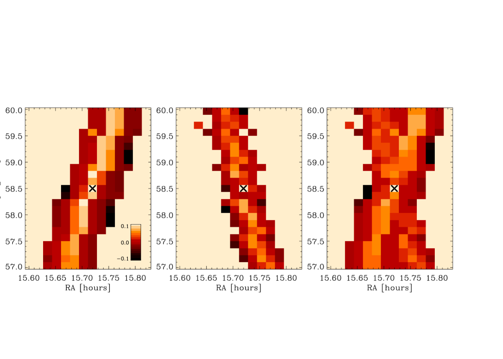
Figure 13: Pixel domain correlations of the noise projected on the sky. All three panels show a level of the correlations relative to the RMS value of the noise for the same pixel, which is marked with an ‘x’. Color coding is shown in left panel. This pixel has been observed twice during the maxima-i flight. The noise correlations for the first observation are shown in the left panel, and these for the second one in the middle panel. Right panel shows the final co-added noise correlations (see Eq. 46). Clearly, due to the maxima-i scanning strategy and the presence of the noise correlations in the time domain, the noise correlation pattern in pixel domain is highly anisotropic and strongly correlated as a result of any single observation of a pixel. The combined noise, for all pixels which were observed twice, is however significantly less correlated and more isotropic.

The map-making formalism as presented so far can be applied to a number of statistically independent segments simultaneously. However, it may be advantageous to analyze each of these separately. In this case one needs to combine the separate segments together at the end. For Gaussian noise this would be quite straightforward, were it not for arbitrariness in the offset of each segment. The latter introduces possible relative offset shifts between the segments. This can be resolved for partially overlapping segments if we require them to display, within the noise uncertainty, the same underlying pattern in the common region. This introduces an extra complication to the well-known formula (e.g., daCosta1999 ) for the optimal co-addition of two maps. The maximum-likelihood problem can be solved in a standard manner or using an approach analogous to that of Sect. IV.2. In consequence, on defining, for each time-stream segment, $u_{p\left(I\right)}$ as a pixel-domain vector of ones and ${\hbox{\boldmath$\hat{u}_{p\left(I\right)}$\unboldmath}}\equiv{\hbox{\boldmath$N_{p\left(I\right)}$\unboldmath}}^{-1}{\hbox{\boldmath$u_{p\left(I\right)}$\unboldmath}}$, and introducing a corrected inverse noise correlation matrix, ${\hbox{\boldmath$N^{\prime}_{p\left(I\right)}$\unboldmath}}^{-1}$, such as (cf., Eqs. 30, 43),

$${\hbox{\boldmath$N^{\prime}_{p\left(I\right)}$\unboldmath}}^{-1}\equiv{\hbox{\boldmath$N_{p\left(I\right)}$\unboldmath}}^{-1}-\frac{{\hbox{\boldmath$\hat{u}_{p\left(I\right)}$\unboldmath}}\otimes{\hbox{\boldmath$\hat{u}_{p\left(I\right)}$\unboldmath}}^{T}}{{\hbox{\boldmath$u_{p\left(I\right)}$\unboldmath}}^{T}{\hbox{\boldmath$\hat{u}_{p\left(I\right)}$\unboldmath}}},$$ (45)

we can express a final full map and a corresponding noise correlation matrix in a familiar manner,

$$N_{p}^{tot} = \left\{\sum_{I}{\hbox{\boldmath$N^{\prime}_{p\left(I\right)}$\unboldmath}}^{-1}\right\}^{-1},$$ (46)

$$m_{p}^{tot} = {\hbox{\boldmath$N_{p}$\unboldmath}}^{tot}\sum_{I}{\hbox{\boldmath$N^{\prime}_{p\left(I\right)}$\unboldmath}}^{-1}{\hbox{\boldmath$m$\unboldmath}}_{\left(I\right)}.$$ (47)

Here the sum is over maps of all segments to be combined. As discussed above the undetermined absolute offsets of each of the segments separately is reflected in the singularity of each of the redefined inverse noise correlation matrices, ${{\hbox{\boldmath$N^{\prime}_{p\left(I\right)}$\unboldmath}}}^{-1}$. The final inversion in Eq. (46) again has to be understood as in Eq. (42) and the singularity needs to be accounted for in subsequent stages of the data analysis, as, for instance, shown in Eq. (43).

A maxima-i based example of an application of this procedure is shown in Fig. 13. As in the case of a single continuous time stream segment Tegmark1997design , re-observing the same patch of the sky along the different scanning direction not only suppresses the level of the noise per pixel but also weakens and isotropizes the correlation pattern in pixel domain.

Note that the expression in the curly brackets of Eq. (46) becomes singular also, if not every segment map is connected (directly or through the number of intermediaries) with the others. If no such link exists the relative offset of such a segment map with respect to the rest of the map remains unknown giving rise to a singular mode in addition to the one related to the absolute offset. However, Eqs. (46) & (47) can still be applied if the inversion of the singular matrix is interpreted as in Eq. (42). The singular eigenvector $v_{p}$ has to now be appropriately replaced.

For instance, in a case of a single disjoint segment the two singular modes emerging as a result of the unknown total offset of the full map and a relative offset of the disjoint part can be chosen as having ones for every pixel belonging to one disjoint part and zeros elsewhere (or vice verse). With the inversion now described by the straightforward generalization of Eq. (42) for the case of multiple singular eigenvectors, the final product of the operation given by Eq. (47) can be a map composed of many disconnected regions with the uncertainty due to our ignorance of their relative offsets incorporated into the total noise correlation matrix, $N_{p}^{tot}$, as given by Eq. (46).

Numerically one may encounter nearly singular cases whenever the overlapping region between two segments is too limited or the noise per pixel in the overlapping area too high to provide any useful constraint on the free offset. A practical and safe way of dealing with such a problem is to reject a (small by assumption) number of common pixels to make a given part genuinely disconnected and to account in a mathematically strict manner for the arising singularity of the noise correlation matrix.

A power spectrum of such an unconnected map can be subsequently computed as explained in Sect. IV.3. However, that requires more involved algebra than that currently implemented in the MADCAP version of the quadratic estimator. For that reason we have rejected all the disconnected segments from the maxima-i maps while computing their power spectra. In that way the number of segments used for the final analysis decreased to 14 per detector Hanany2000 ; Lee2001 .

IV.5 Combining maps of different photometers.

The additional difficulty here in comparison with the previous Section is introduced by the possible relative calibration difference between maps produced for different detectors. Calibration uncertainty is generically difficult to be included into a maximum likelihood framework due to its multiplicative character. For the maxima-i data set we have found that the relative calibration between different photometers’ maps are with a high precision correct if the mean dipole based calibration is adopted for each of the maps Stompor2001b . Therefore rather than seeking a general solution to the problem, we combined maps as given by the Eq. (47) and used the largest single detector error for the calibration uncertainty of the combined map.

IV.6 Low-$\ell$ aliasing.

A potential bias of the final anisotropy power spectrum (but also for other statistics, see, e.g., Cayon2001 ) resulting from this kind of the data analysis is due to an incomplete (and modest in a case of all balloon-borne experiments) sky coverage. That induces the correlation between otherwise uncorrelated (for a statistically isotropic sky) $\ell$ modes. As a consequence, power contained in the low-$\ell$ modes beyond the detection capability can leak to the higher $\ell$ modes which are to be estimated. Because the amplitude of the anisotropy power spectrum usually decays with increasing $\ell$ – and is many orders of magnitude higher in monopole and dipole than in any other mode – there is a potential for biasing of the low-$\ell$ end of the estimated power spectrum.

One possible approach is to consider the unwanted modes as pixel-space templates as discussed above (Sect. IV.3): ${\hbox{\boldmath$v_{p}$\unboldmath}}\left(i_{p}\right)=Y_{\ell m}(i_{p})$ for all the $(\ell,m)$ modes to be marginalized over. ($i_{p}$ is here a pixel number.) We then explicitly marginalize over them, while estimating, e.g., the anisotropy power spectrum (Eq. 43). This is closely analogous to the time stream frequency marginalization of Sect. IV.2.

Another, approximate, way to deal with the problem also can be applied directly on the power spectrum estimation stage is implemented in the MADCAP package Borrill1999mad ; Borrill2000 as described at the end of this Section.

An alternative exact solution is based on Górski’s idea Gorski1994 . In this approach the unwanted low-$\ell$ modes are removed from the map prior to further statistical analysis and the corresponding noise correlation matrix in pixel domain is appropriately corrected to account for the additional uncertainty. Unlike the other just-mentioned options this method produces a ‘cleaned’ version of the sky map to be used henceforth.

Let us start by defining a scalar product of two functions $f$ and $g$ defined at each pixel $i_{p}$ of our map $m_{p}$ as (hereafter $\star$ stands for a complex conjugate),

$$\left({\hbox{\boldmath$f$\unboldmath}}|{\hbox{\boldmath$g$\unboldmath}}\right)\equiv\frac{1}{n_{pix}}\sum_{i_{p}}{\hbox{\boldmath$f$\unboldmath}}^{\star}\left(i_{p}\right){\hbox{\boldmath$g$\unboldmath}}\left(i_{p}\right).$$ (48)

Also we denote by $\left\{{\hbox{\boldmath$y$\unboldmath}}\right\}$ a subset of the $\left(\ell_{0}+1\right)^{2}$ spherical harmonics of the order not higher than $\ell_{0}$ which are to be removed form the map. In general $\left\{{\hbox{\boldmath$y$\unboldmath}}\right\}$ is neither a linearly independent nor a complete basis on the map $m_{p}$. However, we can construct a set of orthonormal functions $\left\{{\hbox{\boldmath$\psi$\unboldmath}}\right\}$ spanning the space of the spherical harmonics included in $\left\{{\hbox{\boldmath$y$\unboldmath}}\right\}$. The construction can be performed by using Singular Value or Cholesky decomposition of the Kowalewski-Gram determinant of $\left\{{\hbox{\boldmath$y$\unboldmath}}\right\}$ functions (as, e.g., Gorski1994 ) and rejecting all the singular modes. The resulting set of functions though orthonormal is clearly not complete. To achieve completeness we can supplement it with the functions from the another orthonormal (and complete) set of functions defined on the map and retain from the latter – through a standard Gram-Schmidt orthonormalization procedure – only those functions (or their linear combination) which are orthogonal to all the $\left\{{\hbox{\boldmath$\psi$\unboldmath}}\right\}$ functions. Practically, that part of the procedure can be encoded using Singular Value Decomposition. A convenient choice of the extra complete functional basis is just a pixel basis, $\left\{{\hbox{\boldmath$p$\unboldmath}}\right\}$,

$${\hbox{\boldmath$p_{\left(i\right)}$\unboldmath}}\left(j_{p}\right)\equiv\delta^{K}\left(i,j_{p}\right),\mbox{where }i,j_{p}=1,...,n_{pix}.$$ (49)

On the successful completion of the entire procedure we end up with the set of the $n_{pix}$ orthonormal functions. By construction, all the $\left\{{\hbox{\boldmath$\psi$\unboldmath}}\right\}$ functions are included in the final basis, and they span all the spherical harmonics of the order $\leq\ell_{0}$ on the map $m_{p}$. Hence all the remaining functions of the final basis (denoted hereafter $\left\{{\hbox{\boldmath$\xi$\unboldmath}}\right\}$), which are orthogonal to the functions $\psi$ by construction, are also orthogonal to the all spherical harmonics of that order.

Algebraically the described procedure consists of a pair of linear transformations, which in a pixel representation can be written down as,

$$\psi \equiv {\hbox{\boldmath$K$\unboldmath}}{\hbox{\boldmath$y$\unboldmath}},$$ (50)

$$\xi \equiv L p$$ (51)

Here $K$ changes the basis from that of spherical harmonics, $\left\{{\hbox{\boldmath$y$\unboldmath}}\right\}$, to $\left\{{\hbox{\boldmath$\psi$\unboldmath}}\right\}$. $L$ transforms the pixel basis, $\left\{{\hbox{\boldmath$p$\unboldmath}}\right\}$, to the orthogonal basis made of basis vectors either parallel or perpendicular to $\left\{{\hbox{\boldmath$\psi$\unboldmath}}\right\}$ and retains only the latter subset, $\left\{{\hbox{\boldmath$\xi$\unboldmath}}\right\}$. These functions complement $\left\{{\hbox{\boldmath$\psi$\unboldmath}}\right\}$ and both sets together form an orthonormal and complete basis $\left\{{\hbox{\boldmath$\psi$\unboldmath}},{\hbox{\boldmath$\xi$\unboldmath}}\right\}$ on the map, such as

$$\left({\hbox{\boldmath$y$\unboldmath}}|{\hbox{\boldmath$\xi$\unboldmath}}\right)=0.$$ (52)

The map purged of all the contribution from the low ($\leq\ell_{0}$) order spherical harmonics is then given as,

$${\hbox{\boldmath$m^{\prime}_{p}$\unboldmath}}=\sum_{j}\left({\hbox{\boldmath$m_{p}$\unboldmath}}|{\hbox{\boldmath$\xi_{\left(j\right)}$\unboldmath}}\right){\hbox{\boldmath$\xi_{\left(j\right)}$\unboldmath}},$$ (53)

and is therefore uniquely represented by a vector $m_{\xi}$ defined as,

$${\hbox{\boldmath$m_{\xi}$\unboldmath}}\left(i\right)\equiv\left({\hbox{\boldmath$m_{p}$\unboldmath}}|{\hbox{\boldmath$\xi_{\left(i\right)}$\unboldmath}}\right).$$ (54)

The total (signal plus noise) correlation matrix for $m_{\xi}$ is then given as,

$$\langle{\hbox{\boldmath$m_{\xi}$\unboldmath}}\otimes{\hbox{\boldmath$m_{\xi}$\unboldmath}}^{T}\rangle=\left[{\hbox{\boldmath$L$\unboldmath}}\left({\hbox{\boldmath$S_{p}$\unboldmath}}+{\hbox{\boldmath$N_{p}$\unboldmath}}\right){\hbox{\boldmath$L$\unboldmath}}^{T}\right],$$ (55)

where $\langle...\rangle$ denotes an ensemble average. $S_{p}$ and $N_{p}$ are signal and noise correlation matrices computed for the complete map, $m_{p}$, prior to any mode removal, i.e., ${\hbox{\boldmath$S_{p}$\unboldmath}}+{\hbox{\boldmath$N_{p}$\unboldmath}}\equiv\langle{\hbox{\boldmath$m_{p}$\unboldmath}}\otimes{\hbox{\boldmath$m_{p}$\unboldmath}}^{T}\rangle$. If the sky signal contains only CMB anisotropy then the signal term, $S_{p}$, is given by,

$${\hbox{\boldmath$S_{p}$\unboldmath}}=\frac{1}{4\pi}\sum_{\ell}{\hbox{\boldmath$P_{\ell}$\unboldmath}}\left(2\ell+1\right)C_{\ell},$$ (56)

where $C_{\ell}$ is the power spectrum of the CMB fluctuations, and $P_{\ell}$ denote matrices of the Legendre polynomials computed for all the pairs of the pixels in the given map, i.e.,

$${\hbox{\boldmath$P_{\ell}$\unboldmath}}\left(i_{p},j_{p}\right)\equiv P_{\ell}\left[\cos\left({\hbox{\boldmath$\gamma$\unboldmath}}\left(i_{p}\right)\cdot{\hbox{\boldmath$\gamma$\unboldmath}}\left(j_{p}\right)\right)\right].$$ (57)

Here ${\hbox{\boldmath$\gamma$\unboldmath}}\left(i_{p}\right)$ is a unit vector pointing at the center of the pixel $i_{p}$ and $P_{\ell}$ a standard Legendre polynomial of an order $\ell$.

The correlation matrix of the map without low-$\ell$ modes, as defined in Eq. (55), can also be rewritten as a sum of a noise-like, $N_{\xi}$, and signal-like, $S_{\xi}$, term,

$${\hbox{\boldmath$L$\unboldmath}}\left[{\hbox{\boldmath$S_{p}$\unboldmath}}+{\hbox{\boldmath$N_{p}$\unboldmath}}\right]{\hbox{\boldmath$L$\unboldmath}}^{T}={\hbox{\boldmath$S_{\xi}$\unboldmath}}+{\hbox{\boldmath$N_{\xi}$\unboldmath}}$$ (58)

Furthermore, on introducing the redefined Legendre polynomials matrices ${\hbox{\boldmath$P^{\prime}_{\ell}$\unboldmath}}\equiv{\hbox{\boldmath$L$\unboldmath}}{\hbox{\boldmath$P_{\ell}$\unboldmath}}{\hbox{\boldmath$L$\unboldmath}}^{T}$ and using Eq. (56), we can rewrite the signal part of Eq. (58) as,

$$S_{\xi} = \frac{1}{4\pi}\sum_{\ell}{\hbox{\boldmath$L$\unboldmath}}{\hbox{\boldmath$P_{\ell}$\unboldmath}}{\hbox{\boldmath$L$\unboldmath}}^{T}\left(2\ell+1\right)C_{\ell}$$

$$= \frac{1}{4\pi}\sum_{\ell}{\hbox{\boldmath$P^{\prime}_{\ell}$\unboldmath}}\left(2\ell+1\right)C_{\ell}.$$

The last equation shows that the signal correlation matrix of the ’cleaned’ map is related to the angular power spectrum of the CMB anisotropies, $C_{\ell}$, in a way which is formally identical to that for the complete map, cf., Eq. (56). Therefore we can use usual quadratic estimator algorithms and, in particular, the MADCAP package Borrill1999mad ; Borrill2000 to estimate the CMB power spectrum having at disposition only the map (and the corresponding noise correlation matrix, Eq. 58) with low-$\ell$ modes removed. To use that package in this case one just needs to replace matrices $P_{\ell}$ (which constitute an intermediate output of MADCAP) with matrices $P^{\prime}_{\ell}$ and use the cleaned map in the $\xi$ representation, $m_{\xi}$, and the noise correlation matrix, $N_{\xi}$, as an input, instead of usual $m_{p}$ and $N_{p}$.

Though the matrices $K$ and $L$ can be chosen to be sparse (nearly triangular) the entire procedure is quite involved and the computational cost scales as ${\cal O}\left(n_{pix}^{3}\right)$. The same scaling applies to the computations of products of $L$ and $P_{\ell}$ matrices. However, while only the low $\ell$ part of the angular power spectrum is likely to be affected by that kind of aliasing, the results of such a test applied to a map with relatively large pixels can provide a useful estimate of the size of the expected effect. In the maxima-i case we applied this test to the map with $10^{\prime}$ pixels (i.e., less than $4000$ pixels in total) and compared it with the simple approximate template procedure of BJK1998 as implemented in the MADCAP package of weighing out the monopole and dipole from the map, and introducing an extra low-$\ell$ bin to the recovered anisotropy power spectrum which is a posteriori rejected. In the maxima-i case this bin extended from $\ell=2$ up to $\ell=34$. Its rejection corresponds to the marginalization over that bin power and would be formally strict only if the likelihood for the power spectrum bin amplitudes were precisely Gaussian. Though such an approach is less general, because of these approximations and because it explicitly assumes the isotropy of the sky signal in the rejected modes, we found no difference between the results of both methods. Therefore, we conclude that the maxima-i final anisotropy power spectrum, in the published to date range of multipoles, $35\lower 2.15277pt\hbox{$\;\buildrel<\over{\sim}\;$}\ell\lower 2.15277pt\hbox{$\;\buildrel<\over{\sim}\;$}1235$, is not affected by any appreciable contribution due to aliasing of the low-$\ell$ mode power.

V Iterative noise estimation.

Figure 14: Estimated noise power spectra for simulated and real data using the iterative approach of Ferreira & Jaffe Ferreira2000 . In left panel, dashed line shows a noise power spectrum computed as in Sect. II.3 without iterative corrections. The dotted line depicts the noise spectrum used for a simulation, that almost perfectly overlaps with a solid line corresponding to a noise power spectrum calculated using 4 iterative steps and a map with 8’ pixels. The dash-dotted line shows a result after 4 iteration but using a map with 3’ pixels. That demonstrates the bias as described in the text. Middle panel shows noise power spectra for a single segment of the actual maxima-i data. The power spectrum has been recovered using various approaches as in the left panel: the solid line shows the spectrum computed with 4 iterative steps and 8’ pixels, dashed line shows the uniterated estimate, and dash-dotted line shows a result of 4 iterative steps with 3’ pixels. The right panel shows noise spectra obtained just as a result of averaging on the second step of the noise estimation procedure, prior to any smoothing (see Sect. II.3 and the right most panel of Fig. 5). Dashed line corresponds to a spectrum obtained with no iteration, displaying characteristic two small spikes at $\sim 0.45$Hz and $0.9$Hz corresponding to a primary mirror chop frequency and its first harmonic. The overplotted solid line is a spectrum after 4 iteration using 8’ pixels. Clearly in the latter spectrum the spikes are corrected as a result of iterations.

To date maxima is one of the most sensitive experiments in terms of the noise level per measurement achieving the level of $\sim 1500\mu$K, i.e., $100\mu\mbox{K}\sqrt{\mbox{s}}$, for some of the detectors. In spite of that the expected CMB and foreground signal for the observed patch of sky is still expected to be a sub-dominant part of a single measurement ($\ll 10\%$ of the total power). The sky-related contribution to the power confined within some of the frequency bands can be, however, much higher ($\lower 2.15277pt\hbox{$\;\buildrel<\over{\sim}\;$}10\%$). Similarly, the non-stationary effects, though they may appear to be quite small, they can be limited to a number of narrow frequency bands, dominating the power in there. For instance, in the maxima-i case the primary mirror synchronous signal with its amplitude of $200\mu$K dominates occasionally the power in the narrow frequency bands centered on the fundamental mode of primary mirror chop and its few lowest harmonics (see Fig. 14).

The important assumption behind the noise power spectrum estimation as presented in Sect. II.3, i.e., that noise dominates the time stream measurements, though not clearly breached needs to be, therefore, tested.

To account for that effect we follow the iterative approach of Ferreira2000 . It attempts to recover the noise component of the entire time stream, which is subsequently used in the noise estimation procedure (see Sect. II.3). The starting point of the iterative procedure is an approximation that ${\hbox{\boldmath$n_{t}$\unboldmath}}^{\left(0\right)}\simeq{\hbox{\boldmath$d_{t}$\unboldmath}}$. Given this, it proceeds to the noise estimation and then to the map making. The resulting (zeroth order) map is used as an estimate of the signal in the time stream and is subtracted from the time stream on the next iterative step Ferreira2000 ; Prunet2000 . If we denote the noise contribution to the time stream on the $i$th step as ${\hbox{\boldmath$n_{t}$\unboldmath}}^{\left(i\right)}$ then,

$${\hbox{\boldmath$n_{t}$\unboldmath}}^{\left(i\right)}={\hbox{\boldmath$d$\unboldmath}}-{\hbox{\boldmath$A$\unboldmath}}{\hbox{\boldmath$m$\unboldmath}}^{\left(i-1\right)}-{\hbox{\boldmath$B$\unboldmath}}{\hbox{\boldmath$x$\unboldmath}}^{\left(i-1\right)}={\cal{A}}^{\left(i-1\right)}{\hbox{\boldmath$\hat{m}_{p}$\unboldmath}}^{\left(i-1\right)},$$ (60)

where ${\hbox{\boldmath$m$\unboldmath}}^{\left(i-1\right)},{\hbox{\boldmath$x$\unboldmath}}^{\left(i-1\right)}$ and ${\hbox{\boldmath$\hat{m}_{p}$\unboldmath}}^{\left(i-1\right)}$ are a map and a primary mirror signal and a generalized map respectively as estimated on the previous step. As shown by  Ferreira2000 the differences between the maps and noise correlation matrices estimated on the subsequent steps of the iteration decrease very quickly and the required precision is achieved rather rapidly. Usually we have found that at most four iterative steps were needed to reach the accuracy of few percent. The iterative approach can be significantly sped up if no explicit inversion of the pixel-pixel noise correlation matrix is performed on each iterative step but the map is calculated using an iterative linear system solver  Prunet2000 ; Prunet2001 ; Dore2001a .

It is important to notice that the method is only asymptotically, – i.e., in the limit of the large number of effective degrees of freedom – unbiased as guaranteed by its maximum likelihood origin. That limit is achieved, for instance, when a number of time samples increases, but a number of pixels is fixed.

The ensuing bias can be estimated as follows. Let us assume that we know the noise correlation function, $N_{t}$. Though the noise estimation goal seems to have been achieved, the iteration, as given by Eq. (60), can go on. The time stream estimate on the next step will contain noise only but composed of two components: a true time stream noise ${\hbox{\boldmath$n_{t}$\unboldmath}}={\hbox{\boldmath$n_{t}$\unboldmath}}^{\left(i\right)}$ and a pixel domain noise, $n_{p}$, projected back to the time domain via the pointing matrix (and therefore also non-stationary):

$${\hbox{\boldmath$n_{t}$\unboldmath}}^{\left(i+1\right)}={\hbox{\boldmath$n_{t}$\unboldmath}}^{\left(i\right)}-{\cal A}{\hbox{\boldmath$n_{p}$\unboldmath}}={\hbox{\boldmath$n_{t}$\unboldmath}}-{\cal A}{\hbox{\boldmath$n_{p}$\unboldmath}}.$$ (61)

The correlations of the latter quantity are computable and given by

$$\left\langle{\hbox{\boldmath$n_{t}$\unboldmath}}^{\left(i+1\right)}\left(i_{t}\right){\hbox{\boldmath$n_{t}$\unboldmath}}^{\left(i+1\right)}\left(j_{t}\right)\right\rangle={\hbox{\boldmath$N_{t}$\unboldmath}}\left(i_{t},j_{t}\right)$$ (62)

$$-\sum_{i_{p},j_{p}}{\cal A}\left(i_{t},i_{p}\right){\cal N}_{p}\left(i_{p},j_{p}\right){\cal A}^{T}\left(j_{t},j_{p}\right).$$

Here the summation is over all pairs of pixels and ${\cal N}_{p}$ stands for the noise correlation matrix in the (generalized) pixel domain corresponding to the true noise correlation in time domain $N_{t}$. $\langle...\rangle$ denotes an average over the statistical ensemble of the noise realizations.

Interestingly, due to existing correlations between noise in the time and pixel domain ‘adding’ the extra noise to the time stream as described by Eq. (61) results in the underestimation of the actual noise power in the time domain. Though the above formula does not really help to unbias the procedure it gives a useful criterion of its applicability. For practical use it is useful to consider the overall power suppression due to the bias. Taking the trace of Eq. (62) we get,

$$\sum_{i_{t}}\left\langle{\hbox{\boldmath$n_{t}$\unboldmath}}^{\left(i+1\right)}\left(i_{t}\right){\hbox{\boldmath$n_{t}$\unboldmath}}^{\left(i+1\right)}\left(i_{t}\right)\right\rangle =$$ (63)

$$\sum_{i_{t}}{\hbox{\boldmath$N_{t}$\unboldmath}}\left(i_{t},i_{t}\right) - \sum_{i_{p}}n_{t}\left(i_{p}\right){\cal N}_{p}\left(i_{p},i_{p}\right).$$

Two limiting cases are evident. If each of the pixels is observed once then the noise iteration has no meaning, as we have no means to distinguish between the noise and the sky signal, and its result is fully biased, i.e., the left hand side of the above equation is zero. If there is no correlation in the time domain then pixel noise is just proportional to the number of times a given pixel has been observed. Inserting that into Eq. (63) renders,

$$\frac{1}{n_{s}}\sum_{i_{t}}\left\langle{\hbox{\boldmath$n_{t}$\unboldmath}}^{\left(i+1\right)}\left(i_{t}\right){\hbox{\boldmath$n_{t}$\unboldmath}}^{\left(i+1\right)}\left(i_{t}\right)\right\rangle=\sigma_{t}^{2}\frac{\left(n_{s}-n_{pix}\right)}{n_{s}},$$ (64)

where $\sigma_{t}^{2}$ is a diagonal element of $N_{t}$. This formula, which in the white noise case can be also derived directly from the maximum likelihood considerations, quantifies the introduced fractional bias as equal to $n_{pix}/n_{s}$. If the number of pixels is fixed then in the limit of the increasing number of measurement the bias disappears as expected.

If the correlations in the time streams are not negligible then a similar expression can be concocted with the number of pixels replaced by an ‘effective’ number of the parameters $n_{eff}$, which is to be determined case by case,

$$\frac{1}{n_{s}}\sum_{i_{t}}\left\langle{\hbox{\boldmath$n_{t}$\unboldmath}}^{\left(i+1\right)}\left(i_{t}\right){\hbox{\boldmath$n_{t}$\unboldmath}}^{\left(i+1\right)}\left(i_{t}\right)\right\rangle\simeq\sigma_{t}^{2}\frac{\left(n_{s}-n_{eff}\right)}{n_{s}},$$ (65)

The intuitive meaning of $n_{eff}$ is clear from the expression

$$n_{eff}\equiv\sum_{i_{p}}n_{s}\left(i_{p}\right)\frac{{\cal N}_{p}\left(i_{p},i_{p}\right)}{\sigma_{t}^{2}}$$ (66)

In the maxima-i case $n_{eff}$ is not smaller than $n_{pix}$, and hence correlations tend to increase the bias of the noise iteration procedure.

It is important to notice that due to our assumption of stationarity, the bias depends only on how on average the measurements are divided between pixels and is therefore robust to the presence of the poorly sampled pixels.

From Eq. (63) it is clear that the bias is a result of the noise presence in the pixel domain. It is therefore advantageous to use all available information to minimize the noise of the estimated map, including all the time stream data during which a given patch of the sky has been observed.

In the maxima-i case we have found (Fig. 14) that it is still advantageous to perform noise iterations for pixels as small as 8 arcminutes. For smaller pixels, the resulting map is occasionally too noisy, and the likely bias larger than an expected gain. Therefore, in those cases, we either restrict iterative corrections to deal only with the primary mirror synchronous signal or use noise power spectrum estimates obtained for the 8 arcminute pixels Lee2001 . The latter approach is helpful in correcting for the low-angular-scale power, which should constitute the bulk of the sky signal present in the time stream. However, one may worry that it also introduces spurious correlations at the time lags corresponding to the characteristic crossing time of the big pixel. In practise, we have found that the results rendered by both these approaches are in very good agreement.

Clearly, invoking some kind of a map-denoising method and/or applying on this stage more aggressive filtering can be useful to extend the applicability of iterative noise estimation. We leave this issue for future research.

VI Consistency tests.

Figure 15: Probability distribution functions of the pixel amplitudes for the noise maps computed as a difference of two maps made for two different photometers. The upper row shows the results using prewhitened maps. Their corresponding unprewhitened versions are displayed in the lower row. Histograms show the results for the real data and smooth lines the Gaussian curves with a dispersion equal to one (upper panels) or fitted to best match the actual results. The two right panels show contour plots of the histograms of joint two-dimensional probability distributions of the pixel temperature for two ‘noise’ maps. These were computed as a difference of the sky maps recovered for two independent pairs of the photometers. The lower panel shows the results for the actual maps with the correlated pixel noise, and upper panel for the maps prewhitened prior to histogramming. Concentric ellipses marked with thin solid lines show the Gaussian expectation. Those were computed assuming no correlations between both maps and were discretized the same way as data histograms and setting the dispersions either to unity (upper panel) or to the best fit values (lower panel).

A number of assumptions and approximations are involved in the computations of a map and a corresponding noise correlation matrix, so it is desirable to test the consistency of the final map-making products. Clearly that is difficult for the maps containing still-to-be-determined cosmological contributions without any prior assumptions. However, it can be done for the maps containing just noise. Those can be either the projections on the sky of the so called ‘dark’ bolometers usually incorporated in experiments to track instrumental effects in the data Lee1999 , or just differences of the maps computed for single detectors. If, as expected, the maps recovered for a single photometer contain only the sky signal and the noise, the subtraction removes the sky component leaving a map of the noise only. Under the assumption of Gaussian time stream noise, the noise maps are also Gaussian, and their correlations are given by the noise correlation matrices produced in parallel by a map-making procedure (Sect. III). Any failure to meet such a requirement would suggest either a failure of the basic assumptions or some other problem with the data, the data analysis methods, or both.

The noise maps, due to correlations and inhomogeneity of the noise, are described by the multi-dimensional probability distributions with a number of dimensions equal to a number of pixels $n_{pix}$ of a map under consideration. Therefore, notwithstanding the large number of pixels, a simple histogram of the pixel temperatures is likely to display significant deviations from the 1-dimensional Gaussian distribution even for the truely Gaussian case. To alleviate this problem we first ‘prewhiten’ the map performing a linear transformation in order to decorrelate the measurements in the different pixels of the map,

$${\hbox{\boldmath$w_{p}$\unboldmath}}\equiv{\hbox{\boldmath$N_{p}$\unboldmath}}^{-\frac{1}{2}}{\hbox{\boldmath$m_{p}$\unboldmath}},$$ (67)

here ${\hbox{\boldmath$N_{p}$\unboldmath}}^{-1/2}$ is a ‘square root’ of the noise correlation matrix as estimated from the map-making, satisfying a relation,

$${\hbox{\boldmath$N_{p}$\unboldmath}}^{-1}\equiv{\hbox{\boldmath$N_{p}$\unboldmath}}^{-{1/2}}\left[{\hbox{\boldmath$N_{p}$\unboldmath}}^{-{1/2}}\right]^{T}.$$ (68)

In the following we take ${\hbox{\boldmath$N_{p}$\unboldmath}}^{-{1/2}}$ to be a Cholesky triangular matrix (e.g., Golub1983 ). If the noise correlations are estimated correctly (or at least consistently), then the components of the vector $w_{p}$ (a ‘prewhitened map’) are uncorrelated and their variances are equal to unity. Thus the multi-dimensional problem reduces to the well-defined one-dimensional test. Moreover, if the noise in the pixel domain is Gaussian then each of the components of $w_{p}$ is randomly drawn from the Gaussian 1-dimensional distribution with the unit variance. That is the hypothesis which we test. We apply a one dimensional Kolmogorov-Smirnov test. Its results give an estimate of how often the one point distribution function such as the one actually measured can be obtained from the Gaussian distribution with a unit variance. For maxima-i we have four single-detector maps, giving us six independent difference maps. We test all of these noise maps, finding that the KS significance is always higher than $\sim 10$% and usually as high as $\sim 50-60$%, confirming the very good consistency of our map-making products. The sample of the results is also shown in Fig. 15. Clearly, a histogram of the unprewhitened map shows a significant deviation from the Gaussian curve near the peak (lower, left panel of the figure) and in the tails of the distribution. As anticipated, prewhitening largely resolves the discrepancies, allowing us to recover nearly perfectly Gaussian curves.

Though such KS-like tests usually provide a weak diagnostic, they are powerful consistency tests when passed. Sources of possible failure are abundant. Those can be either problems of the data set like an extra photometer-dependent parasitic signal in the time-stream leaving its imprint in the difference maps, or non-Gaussianity of the time domain noise, or cross-correlation between maps used for the creation of the difference maps. Moreover, the fact that one of our maps was actually made of the data obtained by the photometer centered at a higher frequency ($\sim 240$ GHz) than the others frequency ($\sim 150$ GHz) also suggests the lack of a substantial frequency-dependent sky (e.g., foreground) signal, as expected from the choice of the low contamination contrast patch observed during the maxima-i flight. Alternatively, the source of the problem may lay with the data analysis, such as noise misestimation both in the time domain and pixel domain as a result of the involved approximations. In fact we have found that the results of KS tests depend on the precise map-making procedure we choose to apply to the real data. In particular, we derive somewhat different numbers if, e.g., no noise iteration has been performed, or no primary-mirror-synchronous signal has been removed. In both cases the differences are mainly due to the differences in the long wavelength modes present in the maps, which are the most susceptible to the details of the map-making algorithm. Nevertheless, that shows that the KS test possesses sensitivity which makes it a useful tool in tracking realistic problems in the maps and/or procedure. The KS test can be also applied to the maps with the low-$\ell$ multipoles removed as described in the previous Section. Hence the lack of an indication of the problem with the KS test results is quite encouraging and may serve as a fairly comprehensive validation of the final results.

In addition, for every pair of the noise maps we can consider a two-dimensional probability distribution of two noise maps calculated as differences of two actual single detector maps. Here we use a difference map of the first and second detector, $m_{p\left(12\right)}$, and of the third and fourth, $m_{p\left(34\right)}$ and consider the probability distribution ${\cal P}\left({\hbox{\boldmath$m_{p\left(12\right)}$\unboldmath}},{\hbox{\boldmath$m_{p\left(34\right)}$\unboldmath}}\right)$.

If we assume that the signal detected by different detectors is uncorrelated, the correlation matrix for a pair $\left({\hbox{\boldmath$m_{p\left(12\right)}$\unboldmath}},{\hbox{\boldmath$m_{p\left(34\right)}$\unboldmath}}\right)$ has a block diagonal structure with blocks given by the correlation matrices of each of the difference map separately. Prehwitening in such a case is simply given by,

$$\left[\begin{array}[]{c}{\displaystyle{\hbox{\boldmath$w_{p\left(12\right)}$\unboldmath}}}\\ {\displaystyle{\hbox{\boldmath$w_{p\left(34\right)}$\unboldmath}}}\end{array}\right]\equiv\left[\begin{array}[]{c c}{\displaystyle{\hbox{\boldmath$N_{p\left(12\right)}$\unboldmath}}^{-1/2},}&{\hbox{\boldmath$0$\unboldmath}}\\ {\hbox{\boldmath$0$\unboldmath}},&{\displaystyle{\hbox{\boldmath$N_{p\left(34\right)}$\unboldmath}}^{-1/2}}\end{array}\right]\left[\begin{array}[]{c}{\displaystyle{\hbox{\boldmath$m_{p\left(12\right)}$\unboldmath}}}\\ {\displaystyle{\hbox{\boldmath$m_{p\left(34\right)}$\unboldmath}}}\end{array}\right].$$ (69)

The two dimensional probability distribution ${\cal P}\left({\hbox{\boldmath$w_{p\left(12\right)}$\unboldmath}},{\hbox{\boldmath$w_{p\left(34\right)}$\unboldmath}}\right)$ is then bound to have a unit variance and the Gaussian shape unless the cross-correlation term is indeed present or any of the previously mentioned reasons/assumptions is not fulfilled. The obtained results (right hand panels of Fig. 15) seem to agree well with the expectations and therefore confirming the consistency of our analysis.

VII Summary.

Recent CMB data sets have set new challenges for the data analysis. Problems are related to a sheer size of new data sets and also to a quality of the analysis tools, which can make a full use of increasing power of data.

This paper describes how those challenges were met in the analysis of the maxima-i data set. The successful production of the final results, as published in the recent papers Hanany2000 ; Lee2001 , required us to improve on the existing and develop and test new methods and tools. Though some of them had to be significantly customized to be efficient, the others seem to be of a more general character and applicability extending to data sets as big as that of the forthcoming satellite missions  Map ; Planck .

We have focused here on time ordered data manipulation techniques and map-making algorithms. We have presented a comprehensive, consistent approach allowing us to recover a map of the sky and to estimate its error matrix in realistic circumstances of an actual CMB experiment. The highlights include:

• the time stream noise estimation procedure coupled together with the gap filling method through constrained noise realization;

• an exact version of the map making code;

• the statistically sound methods of dealing with the time stream filtering of contaminated frequencies and time-domain templates.

The entire suite of the methods presented here amounts to a self-consistent approach to building a final map out of smaller parts in an efficient way. The construction can be halted when the largest map lending itself to the statistical analysis (e.g., power spectrum estimation) has been built. Dealing with only subsets of an entire data set seems to be the only efficient way of searching for, understanding and removing any systematic problems.

CPU time-wise, the presented methods are limited by the noise correlation matrix inversion, which requires ${\cal O}\left(n_{pix}^{3}\right)$ operation. This is the price to be paid if no assumption is made about possible symmetries present in the map and a pixel-pixel noise correlation matrix is required. This obstacle may not be insurmountable, even without sacrificing the generality of the approach. In most of the realistic situations such a matrix is expected to be rather sparse. Moreover, from the knowledge of a scanning strategy and characteristic correlation length in the time domain, it can be guessed a priori which matrix elements need to be computed. We leave both issues for further investigation, noting only here that extensive use of a supercomputer and the MADCAP package facilitates computations of the maps containing up to $\sim 40,000$ Lee2001 .

VIII Acknowledgments

RS and SH acknowledge support of NASA Grant NAG5-3941. AHJ and JHPW acknowledge support from NASA LTSA Grant no. NAG5-6552 and NSF KDI Grant no. 9872979. PGF acknowledges support from the RS. BR and CDW acknowledge support from NASA GSRP Grants no. S00-GSRP-032 and S00-GSRP-031. RS also acknowledges help (in Poland) of Polish State Committee for Scientific Research grant no. 2P03D01719. Computing resources were provided by the National Energy Research Computing Center at Lawrence Berkeley National Laboratory. MAXIMA is supported by NASA Grant NAG5-4454 and by the NSF through the Center for Particle Astrophysics at UC Berkeley, NSF cooperative agreement AST-9120005.

References

- (1) Lee, A.T, et al., 1999, Proceedings of the 3K cosmology meetings, astro-ph/9903249
- (2) http://cfpa.berkeley.edu/maxima
- (3) Hanany, S. et al., Ap.J., 2000, 545, L5
- (4) Lee, A.T., et al., 2001, Ap.J., 561, L1
- (5) http://map.gsfc.nasa.gov/
-
(6)
http://astro.estec.esa.nl/SA-general/
Projects/Planck/ - (7) Wright, E.L., 1996, preprint, astro-ph/9612006
- (8) Tegmark, M., 1997, Ap.J., 480, L87
- (9) Tegmark, M., 1997, Phys. Rev. D., 56, 4514
- (10) Oh, S.P., Spergel, D.N., & Hinshaw, G., 1999, Ap.J., 510, 551
- (11) Ferreira, P.G., & Jaffe, A.H., 2000, MNRAS, 312, 89
- (12) Stompor, R., et al., 2000, Proceedings of the Garching meeting ‘Mining the sky’, astro-ph/0012418
- (13) Hinshaw, G., Proceedings of the Garching meeting ‘Mining the sky’, astro-ph/0011555
- (14) Doré, O., Teyssier, R., Bouchet, F.R., Vibert, D., & Prunet, S., 2001, A&A, 374, 358
- (15) Natoli, P., deGasperis, G., Gheller, C., & Vittorio, N., 2001, A&A, 372, 346
- (16) Prunet, S., Netterfield, C.B., Hivon, E., & Crill, B.P., 2000, preprint, astro-ph/0006052
- (17) Tegmark, M., 1997, Phys. Rev. D., 55, 5895
- (18) Bond, J.R., Jaffe, A.H., & Knox, L., 1998, Phys. Rev. D., 57, 2117
- (19) Borrill, J.D., 1999, Phys. Rev. D., 59, 027302
- (20) Szapudi, I., Prunet, S., Pogosyan, D., Szalay, A.S., & Bond, J.R., 2000, Ap.J., 548, L115
- (21) Wandelt, B., Hivon, E., & Górski, 2000, preprint, astro-ph/0008111
- (22) Doré, O., Knox, L., & Peel, A., 2001, Phys. Rev. D, 64, 083001
- (23) Hivon, E., Górski, K.M., Netterfield, C.B., Crill, B.P., Prunet, S., & Hansen, F., preprint, astro-ph/0105302
- (24) Ferreira, P.G., Magueijo, J, & Górski, K.M., 1998, Ap.J., 503, L1
- (25) Wu, J.H.P., 2000, preprint, astro-ph/0012206
- (26) Wu, J.H.P., et al., 2001, Phys. Rev. Lett., 87, 251303
- (27) Cayón, L., et al., 2001, MNRAS, 326, 1243
- (28) http://cfpa.berkeley.edu/ borrill/MADCAP
- (29) Borrill, J.D., 1999, preprint, astro-ph/9911389
- (30) Stompor, R., et al., 2001, in preparation
- (31) Balbi, A., et al., 2000, Ap.J., 545, L5
- (32) Stompor, R., et al., 2001, Ap.J., 561, L1
- (33) Wu, J.H.P., et al., 2001, Ap.J.Supp., 132, 1
- (34) Press, W.H., Tuekolsky, S.A., Vetterling, W.T., & Flannery, B.P.,1992, Numerical Receipes in C, Cambridge University Press
- (35) Hoffman, Y., & Ribak, E., Ap.J., 380, L5, (1991)
- (36) Golub, H., & van Loan, F., 1987, Matrix operations, The Johns Hopkins University Press, Baltimore
- (37) de Oliveira-Costa, A., et al., 1998, Ap.J., 509, L77
- (38) Wright, E.L., Hinshaw, G., & Bennett, C.L., 1996, Ap.J., 458, L53
- (39) Borrill, J.D., Ferreira, P.G., Jaffe, A.H., & Stompor, R., 2000, Proceedings of the Garching meeting ‘Mining the sky’,
- (40) Górski, Ap.J., 1994, 430, L85
- (41) Prunet, S., et al., 2001, Proceedings of the Garching meeting ‘Mining the sky’, astro-ph/0101073