On time-dependent X-ray reflection by photoionized accretion disks: implication for Fe K$\alpha$ line reverberation studies of AGN

Abstract

We perform a first study of time-dependent X-ray reflection in photo-ionized accretion disks. We assume a step-functional change in the X-ray flux and use a simplified prescription to describe the time evolution of the illuminated gas density profile in response to changes in the flux. We find that the dynamical time for re-adjustment of the hydrostatic balance is an important relaxation time scale of the problem since it affects evolution of the ionization state of the reflector. Because of this the Fe K$\alpha$ line emissivity depends on the shape and intensity of the illuminating flux in prior times, and hence it is not a function of the instantaneous illuminating spectrum. Moreover, during the transition, a prominent Helium-like component of the Fe K$\alpha$ line may appear. As a result, the Fe K$\alpha$ line flux may appear to be completely uncorrelated with X-ray continuum flux on time scales shorter than the dynamical time. In addition, the time-dependence of the illuminating flux may leave imprints even on the time-averaged Fe K$\alpha$ line spectra, which may be used as an additional test of accretion disk geometry. Our findings appear to be important for the proposed Fe K$\alpha$ line reverberation studies in lamppost-like geometries for accretion rates exceeding about $\sim 1\%$ of the Eddington value. However, most AGN do not show Helium-like lines that are prominent in such models, probably indicating that these models are not applicable to real sources.

1. Introduction

Broad Fe K$\alpha$ line emission and the so-called reflection “hump” centered around $\sim 30$ keV are thought to be significant observational signatures of the presence of cold matter in the vicinity of the event horizons of accreting black holes in Active Galactic Nuclei (AGN) and Galactic Black Hole Candidates (GBHC). These spectral features result from the X-ray illumination of the surface of optically thick and relatively cold matter (e.g., Basko, Sunyaev & Titarchuk 1974; Lightman & White 1988; White, Lightman & Zdziarski 1988; George & Fabian 1991; Magdziarz & Zdziarski 1995; Poutanen, Nagendra & Svensson 1996). Because the accretion disks which power this class of sources are optically thick and relatively cool they were considered to be the natural sites at which these spectral features are produced; futhermore, it has been suggested that accurate measurements of the properties of these features can be used to determine the properties of the associated accretion disks. For example, the normalization of the reflection component can provide an estimate of the solid angle covered by the accretion disk as seen from the X-ray source, while the precise Fe K$\alpha$ line profile constrains the radial structure of such a disk and the underlying space-time geometry (e.g., Fabian et al. 1989).

Unfortunately, the steady-state line profile depends on many parameters – e.g., the viewing angle, the inner and outer disk radii, and the Fe K$\alpha$ emissivity as a function of radius. It is impossible to constrain the actual values of all of these parameters simultaneously (see, e.g., Nandra et al. 1999 for the example of NCG 3516). Moreover, the line profile itself cannot constrain the mass of the black hole. For this reason, in the absence of telescopes of sufficiently high angular resolution, it is hoped that the degeneracy in the steady-state models can be removed through observations of time variability of the spectral features (Stella 1990, Matt & Perola 1992; Campana & Stella 1993, 1995). Complimentary, this would also set limits on the physical size of the emitting region and hence determine the black hole mass. Reynolds et al. (1999) and Young & Reynolds (2000) suggested that a red-ward moving “bump” in the Fe K$\alpha$ line profile after an X-ray flare would be a robust signature of a maximally rotating Kerr black hole, thus providing information about the black hole properties inaccessible by other means; it is also hoped that similar observations may even be used to test General Relativity in the strong limit (see also Ruszkowski 2000).

Observational facts gathered to date signal that correlated spectral and timing analysis of data should indeed be very fruitful in testing models: almost every time that theories were subjected to observational scrutiny, AGN produced surprizes that required modifications of these theories. For example, in the completely analogous situation of optical and UV AGN line emission, reverbaration mapping campaigns indicated that the size of the Broad Line Region (BLR) is smaller by roughly a factor of ten than previously thought (see Netzer & Peterson 1997 for a review). Correlated Optical – UV (OUV) continuum variability observations have shown the lags between these two bands to be much shorter than those expected on the basis of the prevailing accretion disk models. This led to the (reasonable) suggestion that the correlated O-UV variability ought to result from the reprocessing of X-rays onto the O-UV emitting disks (Krolik et al. 1991), only to be challenged later by correlated OUV-X-ray monitoring campaigns (Nandra et al. 1998; Edelson et al. 2000) that did not show the expected correlations.

A few existing attempts to observe Fe K$\alpha$ line reverberation also provided frustrating results. A search for the Fe K$\alpha$ line response to continuum variations was performed for MCG–6–30–15 (Lee et al. 2000; Reynolds 2000) and NGC 5548 (Chiang et al. 2000). Whereas the continuum X-ray flux was strongly variable on short time scales, the Fe K$\alpha$ line flux did not correlate with it. Vaughan & Edelson (2001) have split the light curve of MCG-6-30-15 into much shorter time intervals than those done by the previous authors – in bins of RXTE orbital sampling period. While Fe K$\alpha$ line flux is found to vary on very short time scales, it is not correlated with the continuum X-ray flux. This behavior is not predicted by any of the aforementioned theoretical papers, and it clearly deserves an explanation.

The purpose of this paper is to study the microphysics of the problem – i.e., the time-dependent photo-ionized X-ray reflection – in greater detail than it has been done so far. The existing theoretical literature on Fe K$\alpha$ line reverberation (Reynolds et al. 1999; Young & Reynolds 2000; Ruszkowski 2000) are based on the assumption that the illuminated gas maintains a constant density, independent of the value of the X-ray flux, a common assumption of pre-year-2000 literature (e.g., Ross & Fabian 1993; Matt, Fabian & Ross 1993, 1996; $\dot{\rm Z}$ycki et al. 1994; Ross, Fabian & Brandt 1996). In this case one is fortunate in that it is possible to formulate a set of rules that determine the emissivity of the line as a function of the instantaneous value of the ionizing flux, a fact which greatly simplifies this extremely complex problem.

However, several other treatments of the static X-ray reflection problem did not use the constant density assumption considering it may be too restrictive or unrealistic (e.g., Basko, Sunyaev & Titarchuk 1974; Raymond 1993; Ko & Kallman 1994; Ró$\dot{\rm z}$ańska & Czerny 1996; Ross, Fabian & Young 1999; Nayakshin, Kazanas & Kallman 2000, NKK hereafter). These authors employed the condition of hydrostatic balance in order to compute (rather than assume) the gas density. The code of NKK was designed for conditions typical of the inner regions of AGN accretion disks and is especially well placed to compare the predictions of these models with those employing constant density. Substantial differences in the reflected spectra were found (see also Ballantyne, Ross & Fabian 2001). The root of these differences can be traced to the presence of a thermal ionization instability (TII) under conditions of constant pressure, previously known from studies of AGN line emitting clouds (e.g., Krolik, McKee & Tarter 1981; see also Field 1965). Because this instability is present only under constant pressure conditions, it is absent when the constant density assumption is imposed. NKK, Done & Nayakshin (2001) and Ballantyne et al. (2001) conclude that the constant density models are not to be trusted. Therefore, the quantitative Fe K$\alpha$ line reverberation pattern may in fact be different from that found by Reynolds et al. (1999), Young & Reynolds (2000) and Ruszkowski (2000), and it is the purpose of this paper to attempt to clarify in which way. We must mention from the outset, however, that because of the extreme computational overhead, we only study local reflection spectra and do not integrate over the entyre disk surface to produce full time-dependent responce of Fe K$\alpha$ line. Our study is thus only an initial step in the right direction and an additional work will be required to calculate the final Fe K$\alpha$ line transfer function.

The main new effect that we find below can be summarized as follows. Within the constant density approach, the ionization state of the illuminated gas is determined mainly by the instantaneous value of the ionization parameter $\xi=4\pi F_{\rm x}/n$, where $F_{\rm x}$ is the the X-ray flux and $n$ is the local gas density. Given that $n$ is assumed to be unchanged, the resulting Fe K$\alpha$ line flux is a function of $F_{\rm x}$ only. All the line reverberation studies to date have made use of this fact (e.g., see §IIa in Blandford & McKee 1982 and §2 in Reynolds et al. 1999).

In the context of hydrostatic balance models, the gas density at each point is calculated from the hydrostatic equilibrium condition (together with ionization and energy balances, and radiation transfer). A change in the X-ray flux will lead to changes in the gas temperature profile, disturbing hydrostatic balance. The latter can be re-established after time $t$ of order of the local dynamical time. During this time the ionized disk structure is out of equilibrium with the incident X-ray flux, and hence the Fe K$\alpha$ line emissivity is not a function of $F_{\rm x}$. In other words, the hydrostatic balance models have a relaxation time scale that is not present in the constant density models, and it is important to understand possible implications of this for the general X-ray reflection problem.

The structure of the paper is as follows. In §2 we establish the important physical quantities and observables that determine the static reflected spectrum in the general case of a photo-ionized reflector, and then discuss which of these can realistically be measured in future Fe K$\alpha$ line reverberation studies. In §3 we estimate time scales of the problem, while in §4 numerical approach and tests are presented. Discussion of the results and their implications for current observations are given in §5, and §6 lists our conclusions.

2. On static X-ray reflection

X-ray emission is a ubiquitous feature of the AGN spectra. It is believed that the X-rays are emitted in a hot corona which is located in the vicinity of the compact object, just as the cooler, optically thin, geometrically thick accretion disks. The proximity of these two distinct components of AGN emission implies that accretion disks are expected to be strongly photo-ionized by the X-rays, the more so the larger the accretion rate is (e.g., Matt et al. 1993, 1996, Nayakshin 2000b). Based on the extensive literature and our own calculations, we find that the following quantities determine the spectrum of the reprocessed X-rays:

(1) The absolute value of the incident X-ray flux around the iron recombination band, $F_{\rm x}$; this is the most important parameter associated with the Fe K$\alpha$ line emission. In the case of neutral reflection, the line emissivity, $F_{\rm line}\propto F_{\rm x}$, and therefore the line EW is constant (unless the spectrum of the reprocessed X-rays is variable).

(2) The value of the locally produced thermal disk emission, $F_{\rm disk}$. The absolute value of ratio $F_{\rm x}/F_{\rm disk}$ affects the temperature of the ionized skin (see Nayakshin & Kallman 2001).

(3) The photon spectral index of the incident radiation, $\Gamma$. George & Fabian (1991) have shown that the EW of the line increases by about a factor of 1.6 as $\Gamma$ decreases from 2.3 to 1.3. For neutral reflection, the physics of this dependence is rather simple – as $\Gamma$ changes, the amount of X-ray photons capable of photo-ionizing the Fe K-shell changes, and so does the EW of the line.

In the case of photo-ionized reflection, the spectral index plays a more prominent role as it also determines the temperature of the line emitting gas (NKK, Ballantyne et al. 2001).

(4) The abundance array for important elements, $A_{Z}$.

(5) The inclination of the disk with respect to the observer, $i$.

(6) The high energy spectral shape. It is commonly argued that this part of the spectrum does not affect much the Fe K$\alpha$ line emission because very few photons in this energy range are responsible for K-shell photoionization. However, under the conditions of hydrostatic equilibrium considered herein, this part of the spectrum is instrumental in the determination of the Compton temperature of the ionized gas and therefore its ionization state, thus impacting significantly the Fe K$\alpha$ emission. See the Appendix where the role of the cut-off energy $E_{c}$ is enunciated through several numerical tests.

Summarizing the foregoing discussion, the line flux is a function of:

$$F_{\rm line}=F_{\rm line}\left[F_{\rm x},\Gamma,E_{c},(L_{\rm disk},A_{Z},i)\right]\;,$$ (1)

where we divided the variables into two groups. The second group of variables (those in the curly brackets) is not expected to vary on short time scales and hence these variables can be considered fixed in Fe K$\alpha$ line reverberation studies. Indeed, $L_{\rm disk}$, the disk thermal luminosity, is clearly the fastest varying parameter out of the second group. It is expected to vary on the disk thermal time scale, which is a factor $\alpha^{-1}$ longer than the disk dynamical time scale. So, unless $\alpha$ is close to unity, $L_{\rm disk}\simeq$ const on the light crossing time scales of the inner disk. On the contrary, we expect the three parameters from the first group to be variable on roughly same time scales on which $F_{\rm x}$ varies. For example, when either the geometry of the X-ray source or its luminosity varies, the heating/cooling balance of the hot gas ought to change as well, affecting values of $\Gamma$ and $E_{c}$.

Equation (1) clearly displays the challenges one would face when analyzing Fe K$\alpha$ line reverberation data: In the case of more than one parameter variations in the ionizing flux properties, the line flux is not a function of any one single parameter but depends on all of them. Therefore, studies of the correlation of the line flux with the continuum flux alone may be insufficient to uniquely determine the physical parameters of the problem and yield model independent conclusions. We will come back to this point in §LABEL:sect:rel.

The high energy rollover is the parameter most difficult to measure on short time scales. To circumvent this problem, one can concentrate on targets that are relatively dim in terms of ratio $L_{\rm x}/L_{\rm Edd}$ (but not in terms of the observed X-ray flux!), since then no strongly ionized skin is expected. Another approach is to pick AGN with $\Gamma>2$. Although we have not presented any tests for these cases, it is obvious that for steep X-ray spectra, the Compton temperature becomes insensitive to the exact value and shape of the high energy roll-over when $\Gamma-2$ is sufficiently large. Even if $E_{c}$ is highly variable, the temperature and the Thomson depth of the skin will be largely independent of its value.

3. Time-dependent photo-ionized reflection: time scales

The problem of static X-ray illumination of an accretion disk involves at least four major physical processes, none of which can be neglected if an accurate solution to the problem is sought. These processes are: (1) the ionization balance for the illuminated gas; (2) the balance of heating and cooling; (3) the hydrostatic balance; and (4) the transfer of the radiation through the slab. If the illuminating radiation field

were constant for a long period of time and then (at time $t=0$ for convenience) changed to a new intensity (spectral shape, etc) level, then each of these four processes will be taken out of equilibrium. It is thus necessary to ask how long it will take to re-establish the equilibrium corresponding to the new ionizing intensity. This time should then be compared to the light travel time across the inner most disk region to see whether the non-equilibrium effects can be important for Fe K$\alpha$ line reverberation studies.

The radiation transfer time scale, $t_{rt}$, is approximately $(1+\tau_{i})\lambda_{i}/c$, where $\tau_{i}$ is the Thomson depth of the ionized layer of material where most of the reflected spectral features are formed, and $\lambda_{i}$ is the spatial extent of this slab. The value of $\tau_{i}$ is a few (see, e.g., Ross & Fabian 1993; NKK), so $t_{rt}$ is only a factor of few longer than the light crossing time $\lambda_{i}/c$. The remaining three time scales were discussed by Krolik, McKee & Tarter (1981; §IIa) for AGN line emitting clouds, and we will simply re-scale their estimates for the ionized skin. These authors found the radiative recombination time scale for a hydrogenic ion of charge $Z$ to be about $1.6\times 10^{8}T_{7}^{3/2}/Z^{2}p_{13}$ sec, where $p_{13}\equiv nT/(10^{13}{\rm cm}^{-3}{\rm K})$ and $T_{7}\equiv T/10^{7}$ K. This time scale is longest in the ionized skin (rather than in the cold dense material below it), because there the gas temperature reaches its maximum while the pressure has its minimum. We can estimate $p_{13}$ from the fact that the ionization parameter in the skin is very high, i.e., $\xi\equiv 4\pi F_{\rm x}/n_{H}\lower 2.15277pt\hbox{$\;\buildrel>\over{\sim}\;$}10^{4}$ (e.g., Ross, Fabian & Young 1999; $F_{\rm x}$ is the ionizing X-ray flux, and $n_{H}$ is hydrogen density). Using $F_{\rm x}\simeq L_{\rm x}/4\pi R^{2}$ where $L_{\rm x}$ is the total disk (or lamppost) X-ray luminosity, and $R$ is the radius under consideration, we obtain

$$t_{\rm rec}\simeq 0.2\,T_{7}^{1/2}\,M_{8}^{2}\,r^{2}\,\xi_{4}\,Z^{-2}\,L_{46}^{-1}\,{\rm s}\;,$$ (2)

where $M_{8}$ is the black hole mass in units of $10^{8}$ solar masses, $r$ is the radius in units of Schwarzschild radius, $R_{S}$, $\xi_{4}\equiv\xi/10^{4}$, and $L_{46}\equiv L_{x}/10^{46}$ erg¹ s^-1. To put this estimate into perspective, one should compare it to the light crossing time, $R/c$:

$$R/c=10^{3}\,r\,M_{8}\;{\rm s}\,.$$ (3)

The hydrostatic time scale, $t_{\rm h}$, is $\lambda_{s}/c_{s}$ where $\lambda_{s}\simeq[4kTR^{3}/GMm_{p}]^{1/2}$ and $c_{s}$ is the sound speed, and hence

$$t_{\rm h}=2^{3/2}\,r^{1/2}R/c\;.$$ (4)

It is worth noticing that this time scale is always longer than the light crossing time.

Finally, the thermal time scale can be shown to be longest on the top of the ionized skin, where heating and cooling are dominated by the Compton scattering. Writing $t_{\rm th}=3m_{e}c^{2}/U_{\rm rad}c\sigma_{T}$, where $\sigma_{T}$ is Thomson cross section, and $U_{\rm rad}\sim F_{\rm x}/c$ is the radiation energy density, we have

$$t_{\rm th}\simeq\frac{3}{2}r\frac{m_{e}}{m_{p}}\dot{m}_{x}^{-1}R/c\;,$$ (5)

where $\dot{m}_{x}=L_{x}/L_{\rm Edd}$. Note that if $r\sim 10$ and $\dot{m}_{x}\lower 2.15277pt\hbox{$\;\buildrel<\over{\sim}\;$}10^{-2}$, then this time scale can be longer than the light crossing time scale. Fortunately, for such low values of $\dot{m}_{x}$, the Thomson depth of the skin is small (see, e.g., Nayakshin 2000a) and thus the existence of the skin is not important: the reflector is effectively cold. Thus, in practical terms, it is reasonable to fix our attention on the cases when $t_{\rm th}\ll R/c$.

Let us now review these simple estimates in the light of efforts to measure Fe K$\alpha$ line reverberation in AGN. Unless the observer is exactly pole-on and the X-ray luminosity is a Dirac $\delta$-function in time, one always samples emission from a range of radii. Variability of the signal over time scales less than $R/c$ will be difficult to measure, so that it only makes sense to talk about variability on time scales longer than the light crossing time. According to the foregoing discussion, we have

$$\pmatrix{t_{\rm rt}\cr t_{\rm rec}\cr t_{\rm th}\cr}\ll\frac{R}{c}\ll t_{\rm h}\;.$$ (6)

The general problem of the time-dependent X-ray illumination of accretion disks can be solved assuming that the radiation field, ionization and thermal balances adjust to the new value of the ionizing flux instantaneously, but the gas density is to be found from gas dynamical equations rather than from the hydrostatic balance condition.

4. Tests

4.1. Setup

In the previous section, we argued that the time-dependent X-ray illumination of accretion disks needs to be studied with a code that performs radiation transfer, ionization and energy balance calculations and also computes the dynamics of the gas. We are not aware of the existence of a code that would include treatments of all of these processes to the level of details needed for Fe K$\alpha$ line reverberation problem. However, we can use the static X-ray illumination code described by Nayakshin, Kazanas & Kallman (2000), which is appropriate for equilibrium situations, to make certain tests that can give us a rough idea of when time-dependence is important and what kind of spectral changes are to be expected.

The tests that we will perform are of two types. In the first one, we study situations in which X-ray flux was at one (static) luminosity state which we will label (i) for time $t<0$, and then switched abruptly to a new state (j) at $t=0$ and remained at this state indefinitely (i,j here are either 1 or 2). Using the static NKK code, we can compute the reflected spectra and the gas density profiles for the states (i) and (j). In addition, according to §3, at time $t_{\rm th}\ll t\ll t_{\rm h}$ we can compute the reflected spectra under the assumption that the gas density profile is still the same as it was in the state (i), but with the new value for the illuminating flux. We will call this state (ij) as it corresponds to the transition from state (i) to (j). It is clearly important to examine whether reflected spectrum (ij) differs from that of states (i) and (j).

The second type of tests that we will perform are less rigorous in the mathematical sense but are not less interesting due to their implications. In particular, we shall build a toy model for the time evolution of the gas density in the illuminated slab when the X-ray flux is variable.

Here and later in the paper, we choose the geometry of the lamppost model, in which the X-ray source with luminosity $L_{x}$ is on the symmetry axis above the plane of the accretion disk at height $h_{x}=6R_{S}$. The dimensionless accretion rate through the Shakura-Sunyaev disk is $\dot{m}=0.03$. The illuminating X-ray spectrum is a power-law with photon spectral index $\Gamma=1.8$ extending to $E_{c}=200$ keV. We further assume that the state 1 produces X-ray luminosity equal to $L_{x1}=0.3L_{d}$, where $L_{d}$ is the total thermal luminosity of the accretion disk. The state 2 is assumed to have $L_{x2}=L_{x1}/2$.

4.2. Reflected spectra immediately after the transition

Flux increase.  Figure 1 shows temperature profiles resulting from the calculation in which the initial state is (2) and the final state is (1). The state (21) is defined to be the transient state which exists for $t\ll t_{\rm h}$ after X-ray flux changed from the state (2) to (1). Immediately after the transition, the Thomson thickness of the skin remains the same, but its temperature increases roughly by a factor of two, quickly adjusting to changes in the radiation field. This increase is easily understood from the fact that the Compton temperature is proportional to $F_{\rm x}$: $T_{c}\propto J_{x}/J_{\rm disk}\propto F_{\rm x}$, when $F_{\rm x}\ll F_{\rm disk}$ (e.g., Nayakshin & Kallman 2001).

Figure 2 shows equilibrium spectra (1) and (2) and also the reflected spectrum of the transient state (21), all for the nearly-face-on viewing angle around Fe recombination band. Note the decrease in the He-like component of the line in the spectrum (21) compared with that of state (2). This is due to higher temperature of the skin which leads to correspondingly higher degree of ionization. The integrated equivalent width of the Fe K$\alpha$ line complex decreases from about 230 eV to 160 eV – a change of roughly 30%.

A slightly different representation of the spectral shape of the reflected radiation is given in Figure 3, where we plot the ratio of the reflected transient spectrum (21) to that of the equilibrium spectrum (2) at two angles, one nearly face-on and the other nearly edge-on. As already noted, the transient spectrum shows a deficit of the intermediate to highly ionized He-like lines when viewed face-on. Viewed edge-on, it displays a lack of He- and H-like lines compared with equilibrium spectrum (2). Note also a reduction in the broad component of the line. This component is due to Comptonization of the line in the skin and is reduced simply because there is less line emitted (and not because Comptonization becomes weaker).

Figure 1.— Temperature profiles for the illuminated layer of the gas: (1) and (2) are computed assuming the hydrostatic balance and the “nominal” values of the X-ray flux, $F_{\rm x}$, (1) and (2), respectively (see text); (12) is computed assuming the same density profile as in (1) but with value of the illuminating flux appropriate for the state (2). Similarly (21) is the same as (12) but for the transition from state (2) to (1). Note that the differences in the temperature profiles are highly significant observationally (see the following figures).

Figure 2.— Reflected face-on spectra for the hydrostatic balance models – (1) and (2), dotted and dashed, respectively, and the transient spectrum (21), shown with the solid line. Note that Fe K$\alpha$ line complex for the latter is distinctly different from that for either state (1) or (2).

Figure 3.— Ratio of the transient reflected spectrum $I_{21}$ to that of the initial state $I_{2}$ for two inclination angles: $\mu=\cos i=0.95$ (face-on; solid curve) and $0.05$ (nearly edge-on; short dashed curve). Note the deficit of the line emission from the medium to highly ionized species of iron for the face-on spectrum and the corresponding decrease in the highly ionized components as well as their Compton-scattered wings for the edge-on spectrum.

Flux decrease.  Let us now consider the opposite case – transition (12) from the “high” luminosity state (1) to the “low” luminosity state (2). The corresponding temperature profile is also shown in Figure 1. It is notable that in the “transient region” – the region with the Thomson depth $0.35\lower 2.15277pt\hbox{$\;\buildrel<\over{\sim}\;$}\tau_{T}\lower 2.15277pt\hbox{$\;\buildrel<\over{\sim}\;$}0.6$ – the state (12) actually occupies the solutions that are thermally unstable, – i.e., they are positioned below the point (c) on the corresponding S-curve (see Fig. 1 in NKK). These solutions are allowed, however, during the transition because the pressure balance is not obeyed and the gas density is basically fixed (on short time scales). At a fixed density, the thermal ionization instability does not operate (see Krolik et al. 1981 and Field 1965).

Figure (4) displays the transient spectrum (12) along with the equilibrium spectra for comparison, while Figure (5) shows the same spectra but in a broader frequency range. Clearly, the transient region yields significant column depths in species from FeXVII to the completely ionized FeXXVII. The line emission from “intermediate” ionization stages, FeXVII to FeXXIII, and the Compton down-scattered He-like line, fills in (somewhat) the gap between the neutral-like component of the line (that comes from the material beneath the ionized skin) and the He-like component.

However, the most striking out-of-equilibrium effect is the increase in the He-like component of Fe K$\alpha$ line. It is the change in the emissivity of this feature that fuels the increase in the overall EW of the line from 185 eV to 341 eV – an increase of about 90%. Clearly, an effect of such a large magnitude is observationally significant. Also, the changes in the soft X-ray band are even more pronounced (Figure 5). Variability in this energy range is driven by variations in the ionization state of Carbon, Nitrogen, Oxygen and Fe L lines. Both figures indicate that, as with the transition (21), the continuum reflected spectrum (12) is also different from either of the two equilibrium reflected spectra.

Figure 4.— Same as Fig. 2 but for the transient state (12) that is shown with the solid curve.

Figure 5.— Same as Fig. 4 but in a broader energy range.

4.3. A toy model for the density evolution of the ionized skin

As we discussed above, in time-dependent situations, the reprocessing gas density (at each point of the slab) is to be determined from the associated gas dynamics, preferably using a gas-dynamical code. In the absence of such a code, we will use the following simple prescription:

$$\frac{\partial\rho(\tau_{T},t)}{\partial t}=-\frac{\rho(\tau_{T})-\rho_{\rm eq}(\tau_{T})}{t_{\rm h}}$$ (7)

where $\rho_{\rm eq}$ is the “equilibrium” state density profile of the illuminated gas [for example, if we are studying the (12) transition, then $\rho_{\rm eq}(\tau_{T})=\rho_{2}(\tau_{T})]$. Note that $\rho_{\rm eq}(\tau_{T})$ is a function of the Thomson depth (as opposed to a constant), which ensures that the correct hydrostatic balance-based solution is reached at $t=\infty$. While equation (7) is admittedly ad-hoc, it mimics several important properties of the density evolution that we expect. Namely, at times $t\ll t_{\rm h}$, the gas density profile is close to that of the initial state; at times $t\gg t_{\rm h}$, $\rho(\tau_{T})=\rho_{\rm eq}(\tau_{T})$; at intermediate times $t\sim t_{\rm h}$ the density profile is a mixture of the initial and final states. In addition, the re-adjustment of the gas density occurs on roughly correct time scales. We plan to calculate the gas dynamics explicitly in our future studies.

4.3.1 Warm skin limit

Nayakshin & Kallman (2001) have shown that the ionization state of the skin and the reflected spectrum are strongly affected by the ratio of the incident X-ray flux, $F_{\rm x}$, to the disk flux, $F_{\rm disk}$. They defined the “warm skin” limit in which the skin is highly but not completely ionized. For hard X-ray spectra, $\Gamma\sim 1.8$ with $E_{c}\lower 2.15277pt\hbox{$\;\buildrel>\over{\sim}\;$}100$ keV, this limit occurs when $F_{\rm x}\lower 2.15277pt\hbox{$\;\buildrel<\over{\sim}\;$}F_{\rm disk}$. Fe K$\alpha$ line emission in this case is dominated by Helium-like Fe at energy $E\simeq 6.7$ keV (unless the skin is Thomson thin). The opposite limit was termed the “hot skin” one: in this case the skin is nearly completely ionized and it is possible to neglect all the atomic processes in the skin. This limit holds for $F_{\rm x}\gg F_{\rm disk}$ (for the same spectra).

Using this setup, we computed time evolution of the gas density and the resulting spectra for transition (21). The calculation was carried out with a time step of $0.1t_{\rm h}$ up to time $t=4t_{\rm h}$. The time-dependent temperature profiles are shown in Figure (6), with numbers labelling the times at which the snapshots were taken. Note that even at $t=4t_{\rm h}$, the temperature and the density profiles still have not reached the “final” equilibrium state. In the “transient” region, i.e., at $0.3\lower 2.15277pt\hbox{$\;\buildrel<\over{\sim}\;$}\tau_{T}\lower 2.15277pt\hbox{$\;\buildrel<\over{\sim}\;$}0.6$, temperature evolves from the cold branch through all the intermediate values to the hot branch. As discussed in §4.2, the gas can temporarily occupy thermally unstable solutions that are forbidden in the equilibrium configurations.

Panel (a) of Figure (7) shows time dependency of the equivalent width (EW) of the integrated Fe K$\alpha$ line profile, while panel (b) displays the EW for the three prominent components of the line – the bins that contain the neutral-like 6.4 keV, the He-like $\sim 6.7$ and H-like $\sim 6.9$ keV components. During the transition, the total EW varies by a factor of 2, far greater than in the spectra obtained in §4.3.1 immediately after the change in the flux from (2) to (1). This is clearly highly significant observationally since the X-ray flux itself was varied by the same amount.

Let us now make a detailed analysis of the spectral evolution. From Figure 6, we observe that at $t\lower 2.15277pt\hbox{$\;\buildrel<\over{\sim}\;$}t_{\rm h}$, the cold layers below the ionized skin are relatively unaffected. Though in part this is due to the simplified treatment of the cold branch of the solution (as described in the footnote to §4.2), we believe this is a general result because the cooling of the cold branch is done mostly through optically thick processes, and hence the cooling function there depends very strongly and non-linearly on temperature. A change in the X-ray flux of the order of 2 will cause only a slight change in the temperature of this region, contrary to the highly ionized skin (where the cooling function depends on the temperature in an approximately linear fashion). In addition, the gas temperature must increase to about $100$ eV, that is about 10 times from its initial value of $8$ eV, in order for the iron to become sufficiently ionized to permit FeXVII and higher ionization species to become dominant line emitters. Therefore, the line emission from this cold region – the neutral-like component at $E=6.4$ keV – evolves very slowly in the beginning of the calculation, as can be seen in panel (b) of Figure (7). Only at $t\lower 2.15277pt\hbox{$\;\buildrel>\over{\sim}\;$}1.5\,t_{\rm h}$, the transient region’s density evolves enough to allow for a substantial warming up of that region and the associated decrease in the neutral-like Fe K$\alpha$ line emission.

The evolution of the Helium-like Fe K$\alpha$ component is dictated by the fact that at first the skin heats up due to the increase in the ionizing flux and therefore the emission from this component significantly decreases. At later times, when the transient region warms up, the He-like emission increases by as much as a factor of 4. The Hydrogen-like component at $E\simeq 6.9$ keV remains very weak and approximately constant during the entire interval, a fact due mostly to the intrinsically low effective fluorescence yield of H-like Fe. Also note that at times $t\sim 1-2t_{\rm h}$, the soft X-ray band exibits many strong lines and recombination continua which we do not show here (cf. Fig. 5; in addition, animations of the temperature and spectral changes can be found at “http://lheawww.gsfc.nasa.gov/users/serg/”).

Figure 6.— Evolution of the temperature profiles for the illuminated layer of the gas during the transition (21) computed under the assumption that the gas density profile evolves as described by equation (7). The curves shown with the stars connected by dashed lines are the equilibrium temperature profiles (1) and (2) [same as in Figure 1]. Subsequent curves are computed for times $t/t_{\rm h}=0.5,1.0,1.5,...,4.0$. The numbers next to the respective curves indicate time.

Figure 7.— (a) Stars – Evolution of the total equivalent width (EW) of the Fe K$\alpha$ line during the transition (21) as viewed at $\cos i=0.95$. Horizontal lines show the EW of the initial and final equilibrium states (1) and (2). Note that EW of the line still evolves at the end of the simulation because the density profile has not completely relaxed after $t=4t_{\rm h}$, and that it will eventually relax to the state (1). (b) “Equivalent Width” of the bins that contain the neutral-like 6.4 keV component of the line, Helium-like component at $\sim 6.7$ keV, and Hydrogen like one at $\sim 6.9$ keV during the transition. The non-linear and non-trivial character of the evolution of the EW with time is obvious.

4.3.2 Hot skin limit

The second test we perform is for the same geometry, but for the ratio of $L_{\rm x}/L_{\rm disk}=3$ in the state (1), and the accretion rate $\dot{m}=3\times 10^{-3}$. The corresponding temperature profiles are presented in Figure 8, while the EW of the line is plotted in Fig. 9. The character of the temperature and spectral evolution during the transition is similar to that of the warm skin limit, except that the He-like line emission suffers even greater variations. This is a consequence of the fact that the skin in state (1) is completely ionized, which means that the He-like line emissivity evolves from virtually zero to being the dominant component and then decaying as the skin approaches the new (hot) state (2).

Figure 8.— Evolution of the temperature profiles for the illuminated layer of the gas during the transition (21) in the hot skin limit (see §4.3.2). The meaning of the curves is the same as in Figure 6]. Subsequent curves are computed for times $t/t_{\rm h}=0.5,1.0,1.5,...,4.0$. The numbers next to the respective curves indicate time.

Figure 9.— Same as Figure 7 but for the hot skin limit. Hydrogen-like line emission at $\sim 6.9$ keV is not shown since it is negligible at all times.

5. Discussion

5.1. Main results and implications for current observations of AGN

Our main results can be summarized as following.

(1) The gas hydrodynamical time, $t_{\rm h}$, is an important relaxation time scale of the X-ray reverberation problem. The hydrostatic equilibrium assumption fails for variations with characteristic time scale $t\lesssim t_{\rm h}$. As shown, this will in general affect the reflected spectra, unless the Thomson depth of the ionized skin is much smaller than unity.

To make this point clearer, we plot (Figure 10) the time profile of the illuminating flux (in slab geometry) and the line emissivity in normalized units for the simulation presented in §4.3.1. It is apparent from this figure that the line flux responded to the change in the illuminating flux only after a delay $t\sim t_{\rm h}$. Therefore, there is a possibility that the slow evolution of the Fe K$\alpha$ line emissivity, caused by the evolution of the ionization state of the reflector, might be mis-interpreted as being due to the specific geometric arrangement or the presence of general-relativistic effects. We will discuss this point a little further in §5.2.

Figure 10.— The continuum X-ray flux and Fe K$\alpha$ line flux as a function of time for transition studied in §4.3.1. Note that the line flux goes up at substantially later time, and this ionization physics effect may be misinterpreted as a geometrical delay.

(2) If the illuminating flux fluctuates on time scales $t\gg t_{\rm h}$, the resulting spectra can be computed in the quasi-static approximation (e.g., NKK). Effectively, this is the limit in which all of the ionized X-ray reflection calculations (of which we are aware) were performed to date.

(3) In the opposite case, $t\ll t_{\rm h}$, the ionized disk is out of hydrostatic equilibrium and the reflected spectra can be significantly different from that obtained under the quasi-static assumption. In particular, the Fe K$\alpha$ line emissivity is not a function of the instanteneous X-ray flux that would have been implied from the hydrostatic models of NKK. The Thomson depth of the skin is approximately that appropriate for the time-averaged X-ray flux, but the transition from highly to weakly ionized layers is not sharp and time-steady as in the models of NKK. The time-averaged reflected spectra are not the same as quasi-static reflected spectra computed for the average incident flux.

This is not surprising if one considers that the response of the disk to the ionizing radiation is a strongly non-linear process driven by the TII. The observed response depends not only on the frequency of variation but also on the initial conditions of the reprocessing matter. Consider, for example, a specific dependence between the X-ray flux and the line equivalent width under steady-state conditions depicted schematically by the thick solid line in Fig. 11 (for realistic examples see Figure 1 of Nayakshin 2000b). For fast flux variations, i.e., those for which changes in $F_{\rm x}$ occur on time scales shorter than $t_{\rm h}$, one will, in general, observe different levels of Fe K$\alpha$ line flux if one arrives at the continuum flux corresponding to point B starting from different initial points (cf. paths A–B_A and C–B_C in the figure). In fact, since the flux variations disturb hydrostatic balance, one will not come back to the initial point on the curve even if the flux attain its original value (see trajectory B–B_B). These curves will converge to the same value of the ordinate only if the X-ray flux did not change from its final value (at point B) for time scales much longer than $t_{\rm h}$. Hence, on short time scales there is no “correct” value for the line flux at a given continuum level and therefore one could obtain no apparent correlation between these two quantities in a monitoring campaign, instead of the one expected on the basis of steady state calculations.

Figure 11.— Schematic drawing of the dependency of line flux on the continuum flux. The thick solid curve shows the equilibrium curve – i.e., one that is obtained for a fixed shape of the illuminating spectrum and assuming hydrostatic balance. Non-equilibrium paths A–B_A, C–B_C, and B–B_B are shown as examples of the “trajectories” allowed under time-dependent conditions. Thus, in non-equilibrium situations, more than one value of the line flux for a given continuum flux is to be expected.

This argument may provide an explanation for the results of the analysis of the Fe K$\alpha$ line variability of MCG 6–30–15 by Vaughan & Edelson (2001): These authors split the X-ray light curve of this object into bins of the RXTE sampling period, i.e. of order of 6000 seconds. They found (see their Figure 3) that the Fe K$\alpha$ line flux was variable on time scales of a few RXTE orbits, but it was not correlated with the continuum flux in any consistent manner.

The parameters associated with this object are roughly consistent with those needed for an explanation of these results as due to the finite value of $t_{\rm h}$. Demanding the value of the latter to be $\simeq 6000$ sec and assuming a “reasonable” value of $r=5$, one obtains (Eq. 4) for the mass: $M\sim 2\times 10^{7}{\,M_{\odot}}$. The observed X-ray luminosity of MCG 6–30–15 is $\sim{\rm a~{}few}\times 10^{43}$ erg s^-1 (e.g., Iwasawa et al. 1996), implying an accretion rate of a few percent or more. Following the results of Nayashin & Kallman (2001) it is expected that the Thomson depth of the ionized skin would be sufficiently large to make the out-of-equilibrium effects significant.

Finally, one should bear in mind that the Fe K$\alpha$ line emissivity of an ionized reflector is a function of the total radiation continuum seen by the reflector and not just the $2-10$ keV part of it typically picked by observers. In fact for spectra with $\Gamma<2$ the $E\lower 2.15277pt\hbox{$\;\buildrel>\over{\sim}\;$}10$ keV part of the spectrum contains most of the X-ray luminosity and thus determines the depth of the ionized skin. Thus, Fe K$\alpha$ line flux and $F_{2-10}$ do not have to be directly related even in the quasi-static case. Variations in this (unobserved) part of the spectrum (see Eq. 1 and the Appendix) might of course be invoked for a more prosaic explanation of the results of Vaughan & Edelson (2001).

5.2. Implications for future Fe K$\alpha$ line reverberation studies

The question of immediate interest following the discussion above is the potential impact of the non-equilibrium effects on the future Fe K$\alpha$ line reverberation campaigns (e.g., see Young & Reynolds 2000). The Thomson depth of the skin is much smaller than unity in the lamppost geometry if $L_{\rm x}\ll 0.01L_{\rm Edd}$, and then the ionized layer is not important altogether. Many AGN are brighter than this, possibly, and for these the non-equilibrium effects ought to be important. However, the calculations presented above are purely local, considering the response of only a small region of the disk in slab geometry. More work is needed to determine whether the local effects will affect the reflected signatures of a full disk. While this complicates the theory of Fe K$\alpha$ line reverberation, we should not forget that with that there comes a new tool (beyond static models) to distinguish between models of different geometric arrangements on the basis of the responce of the reflected spectra to the continuum.

Conceptually the simplest model is that with the lamppost geometry. The X-ray source is stationary and it is the Fe K$\alpha$ line “echo” from different parts of the disk that determines the reflected line profile. An alternative arrangement is that of magnetic flares (Nayakshin & Kazanas 2001). In this geometry the observed $L_{\rm x}$ is the aggregate of the emission of a large number of flares that take part in Keplerian rotation of the disk. Because of the rather limited extent of magnetic structures on the disk, one expects the Fe K$\alpha$ line features to be rather narrow and oscillate in energy space with the Keplerian frequency (Nayakshin & Kazanas 2001; Ruszkowski 2000), properties which may allow future observations of higher energy and time resolution to distinguish them in the X-ray light curves. As long as the narrow features are distinguishable in the spectrum, their magnitudes do not matter in the analysis of the trajectories of the emitting spots, and this is why the complications with the non-equilibrium effects may be circumvented.

5.3. Frequency Resolved Spectroscopy

At this point one should note that the power density spectra of AGN as well as those of GBHCs are power laws which cover a large number of decades in Fourier frequency. In AGN specifically, they extend to very low frequencies ($\lesssim\mu$Hz; Edelson & Nandra 1999), much lower than the characteristic time scales discussed in section 3; therefore, one would expect at some frequency the transition from the $t<t_{\rm h}$ to the $t\gg t_{\rm h}$ regime, with the concommitant change in the correlative properties between the continuum and the Fe K$\alpha$ line.

Perhaps the most efficient way of studying these effects is to implement, when appropriate, the frequency resolved spectroscopy method employed by Revnivtsev, Gilfanov & Churazov (1999) in the spectro-temporal analyis of the data of Cyg X-1 and compare the results to models which incorporate the above discussed processes. In applying their method to the hard state of Cyg X-1, Revnivtsev et al (1999) found that the Fe K$\alpha$ line and reflection features appear to weaken with increasing in Fourier frequency. In particular, these features drop to about half of their value at a frequency $f\sim 10$ Hz, and continue to decline to the highest frequencies probed by their analysis ($f\sim 30$ Hz).

Our models predict that the one-to-one correlation between the X-ray flux and the Fe K$\alpha$ line flux may be broken on short time scales. They do not predict a decrease in the variability of Fe K$\alpha$ line with increasing frequency as such, so the lamppost-like models do not seem to offer any physical explanation for results of Revnivtsev et al (2000).

At the same time, note that the observations also show that the X-ray continuum slope decreases with increasing frequency from about $\Gamma\sim 1.9$, for frequencies below $f\sim 1$ Hz, to $\Gamma\sim 1.6$ for $f\sim 30$ Hz. This is significant, because as shown by NKK, Done & Nayakshin (2001), Ballantyne et al. (2001), with other things being equal, a steepening in the X-ray spectrum lowers the Thomson depth of the skin and its degree of ionization. In particular, when the X-ray spectrum is hard, i.e., $\Gamma\sim 1.7$, the skin is nearly completely ionized so it supresses all the reflection signatures. For $\Gamma\lower 2.15277pt\hbox{$\;\buildrel>\over{\sim}\;$}2$, the skin contains a non-negligible amount of He-like iron, and then the line cannot be completely suppressed, no matter how high the ionizing flux is. These facts incorporated in the observations of Revnivtsev et al. (1999) might hence provide an account for the corresponding behavior of the Fe K$\alpha$ line behavior observed within the framework of the models of NKK, NK and Done & Nayakshin (2001). Clearly the regions processing hard flux should be geometrically distinct from those processing softer flux, which is possible only if these fluxes result from different X-ray sources (e.g., magnetic flares). However, a more definitive statement along these lines will have to await the development of more detailed models.

6. Conclusions

We performed a first, highly simplified, calculation of time-dependent spectra due to X-ray reprocessing on the surface of an accretion disk, assuming a step function variation in the incident X-ray flux and limiting ourselves to their effects on a limited section of the accretion disk which we have treated in the slab approximation. While our treatment of the hydrodynamic response of the photoionized gas density profile to changes in the X-ray flux is admittedly very simple, we nonetheless expect that our qualitative conclusions will hold in a more sophisticated calculation. We found that the time necessary for establishing hydrostatic balance in the X-ray heated skin of the disk is an important relaxation time scale of the problem. Furhtermore, because of the non-linear nature of the optically thick ionized X-ray reflection problem, the “relaxation” process allows for entirely new physical solutions at transient times, absent in the steady-state solutions. One of the new interesting features is the presence of a strong He-like component at $\sim 6.7$ keV of the Fe K$\alpha$ line during a transition from an initial neutral-like to the final neutral-like spectrum.

Because of the presence of this relaxation time scale, under time-dependent conditions, the reflected spectrum is not a function of the instantaneous illuminating flux or other system parameters and depends on the history of variations of these parameters. This fact may provide an explanation for the recent analysis of time-dependent reflection data for MCG-6-30-15 by Vaughan and Edelson (2001). It is also important to note that, because of the non-linear character of the formation of the ionized skin on the surface of the accretion disk, as indicated by our results, the time-integrated spectra of real sources may not always be modelled as static spectra corresponding to the average X-ray luminosity during the observation.

While a definitive asnwer of the effects described above within the specific models should await further more detailed investigations, as argued in section 5.2 they can be important for the for the lamppost models of Fe K$\alpha$ line reverberation of AGN once X-ray luminosity of the source exceeds a percent or so of the Eddington luminosity. Their importance in other such models e.g. the flare models of Ruszkowski (2000) and Nayakshin & Kazanas (2001) is harder to assess because of the additional details that will have to be specified to completely determine these models. Nonetheless, for any given model, these effects are well defined and their incorporation in the analysis of future observations of higher time and energy resolution should provide additional means for discriminating between the various models and hence contribute to probing the physics of accretion in the vicinity of compact objects.

SN acknowledges support from the National Research Council during the bulk of the time devoted to this project. The authors are very grateful to Tim Kallman, Chris Reynolds and Mitch Begelman for discussions and useful comments that improved this paper.

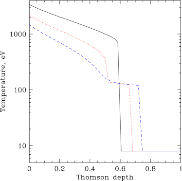
Figure 12.— Temperature profiles of the illuminated gas calculated for the same geometry and total X-ray luminosity, $L_{x}$, etc., with only the high-energy part of the illuminating spectrum varied between the tests. The solid curve shows the temperature profile for the case of a sharp cutoff at $E=200$ keV, while the dotted and the dashed ones show tests with an exponential roll-over at $E_{c}=150$ and $75$ keV, respectively.

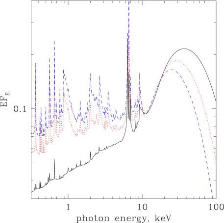
Figure 13.— Reflected spectra for the tests presented in Fig. 12. The meaning of the curves is the same as in Fig. 12.

The importance of the high energy rollover in the spectrum was discussed by Nayakshin & Kallman (2001), but no quantitative tests were presented. Therefore, using the code of NKK, we perform here several tests that validate listing $E_{c}$ as a major unknown. For simplicity, we choose the geometry of the lamppost model with $h_{x}=6R_{S}$ and $\dot{m}=0.01$. The illuminating X-ray spectrum is a power-law with photon spectral index $\Gamma=1.8$. Figure 12 shows the temperature profiles for the illuminated gas for three different shapes of the high energy cutoff. The solid curve shows the reflected spectrum for the case of a sharp cutoff at $E=200$ keV, whereas the dotted and the dashed correspond to tests with an exponential roll-over at $E_{c}=150$ and $75$ keV, respectively. The main effects in the evolution of the temperature profiles, from the sharply cut to the $E_{c}=75$ keV curve, seem to be

Note (1) the decrease in the gas temperature on the top of the skin; (2) an appearance and increase in the extent of the “mid-temperature” step at $kT\sim 150eV$ as $E_{c}$ decreases. The physical mechanism behind the changes in the temperature profiles and the reflected spectra is the change in the photo-ionization equilibrium curve – the so-called “S-curve” (see, e.g., Krolik et al. 1981; Fig. 1 in NKK). As shown by Nayakshin (2000a), the transition between the hot and the cold parts of the ionized gas occurs at the gas pressure

$$P_{\rm gas}\sim P_{\rm crit}=0.032T_{1}^{3/2}\,J/c\;,$$ (1)

where $T_{1}$ is the Compton temperature of the local radiation field, and $J$ is the local radiation energy density. As the high energy cuttoff $E_{c}$ decreases, $P_{\rm crit}$ decreases as well, and this is why there is somewhat less of the ionized skin and it is also cooler for smaller $E_{c}$.

Figure 13 shows the reflected spectra at the inclination angle $\mu=\cos i=0.85$ ($\mu=1$ corresponds to the normal to the disk). The Fe K$\alpha$ line EW changes from about 82 eV to more than 200 eV. Clearly, the variations in the spectra induced by the changes in the cutoff shape are large and non-trivial, and therefore the exact value of $E_{c}$ is indeed important in the determination of the Fe K$\alpha$ line emission from the disk.

References

- (1) Basko, M.M., Sunyaev, R.A., & Titarchuk, L.G. 1974, A&A, 31, 249
- (2) Ballantyne D., Ross, R., Fabian A.C., 2001, MNRAS, in press.
- (3) Blandford, R.D., & McKee, C.F. 1982, ApJ, 255, 419
- (4) Campana, S., & Stella, L. 1993, MNRAS, 264, 395
- (5) Campana, S., & Stella, L. 1995, MNRAS, 272, 585
- (6) Chiang, J., Reynolds, C. S., Blaes, O. M., Nowak, M. A., Murray, N., Madejski, G., Marshall, H. L., & Magdziarz, P. 2000, ApJ, 528, 292
- (7) Done C., Madejski G.M., ycki P.T., 2000, ApJ, 536, 213
- (8) Done, C., & Nayakshin, S. 2000, 546, 419
- (9) Edelson, R. & Nandra, K. 1999, ApJ, 514, 682
- (10) Edelson, R., et al. 1999, ApJ, 534, 180
- (11) Edelson, R. et al. 2000, ApJ, 534, 180
- (12) Esin A. A., McClintock J.E., Narayan R., 1997, ApJ., 489, 865
- (13) Fabian, A.C., Rees, M.J., Stella, L., & White, N.E. 1989, MNRAS, 238, 729
- (14) Fabian, A.C., Iwasawa, K., Reynolds, C.S., & Young, A.J. 2000, PASP accepted (astro-ph/0004366)
- (15) Field G.B., 1965, ApJ, 142, 431
- (16) Galeev, A. A., Rosner, R., & Vaiana, G. S., 1979, ApJ, 229, 318
- (17) George, I.M., & Fabian, A.C. 1991, MNRAS, 249, 352
- Haardt, Maraschi and Ghiselli (1994) Haardt F., Maraschi, L., & Ghisellini, G. 1994, ApJ, 432, L95
- (19) Ichimaru, S. 1977, ApJ, 214, 840
- (20) Kallman, T.R., & White, N. E. 1989, ApJ, 341, 955
- (21) Ko, Y-K, & Kallman, T.R. 1994, ApJ, 431, 273
- (22) Krolik, J.H., McKee, C.F., & Tarter, C.B. 1981, ApJ, 249, 422
- (23) Krolik, J. H., Horne, K., Kallman, T. R., Malkan, M. A., Edelson, R. A., & Kriss, G. A. 1991, ApJ, 371, 541
- (24) Lee, J. C., Fabian, A. C., Reynolds, C. S., Brandt, W. N., & Iwasawa, K. 2000, MNRAS, 318, 857
- (25) Lightman, A.P., & White, T.R. 1988, ApJ, 335, 57
- (26) Magdziarz, P., & Zdziarski, A.A. 1995, MNRAS, 273, 837
- (27) Matt, G., & Perola, G.C., 1992, MNRAS, 259, 433
- (28) Matt, G., Fabian, A.C., Ross, R.R.1993, MNRAS, 262, 179
- (29) Matt, G., Fabian, A.C., Ross, R.R. 1996, MNRAS, 278, 1111
- (30) Nandra, K., George, I.M., Mushotzky, R.F., Turner, T.J., & Yaqoob, T. 1997, ApJ, 488, L91
- (31) Nandra, K., et al. 1998, ApJ, 505, 594
- (32) Nandra K., George I.M., Mushotzky R.F., Turner T.J., Yaqoob T., 1999, ApJ, 523, L17
- (33) Nayakshin, S. 2000a, ApJ, 534, 718
- (34) Nayakshin, S. 2000b, ApJ, 540, L37
- (35) Nayakshin, S., Kazanas, D., & Kallman, T. 2000, ApJ, 537, 833
- (36) Nayakshin, S., & Kallman, T. 2001, ApJ, 546, 406
- (37) Nayakshin, S., & Kazanas, D. 2001, to appear in ApJL, vol 553.
- (38) Netzer, H., & Peterson, B.M. 1997, Astronomical Time Series, Eds. D. Maoz, A. Sternberg, and E.M. Leibowitz, 1997 (Dordrecht: Kluwer), p. 85.
- (39) Poutanen, J., Nagendra, K.N., & Svensson, R. 1996, MNRAS, 283, 892
- (40) Poutanen, J. & Svensson, R. 1996, ApJ, 470, 249
- (41) Quataert, E., & Gruzinov, A. 2000, to appear in ApJ (astro-ph/9908199)
- (42) Raymond, J.C. 1993, ApJ, 412, 267
- (43) Revnivtsev, M., Gilfanov, M., & Churazov, E. 1999, A&A, 347, L23
- Reynolds and Begelman (1997) Reynolds, C.S., & Begelman, M.C. 1997, ApJ, 488, 109
- (45) Reynolds, C.S., Young, A.J., Begelman, M.C., & Fabian, A.C. 1999, ApJ, 514, 164
- (46) Reynolds, C.S., 2000, ApJ, 533, 811
- (47) Ross, R.R., & Fabian, A.C. 1993, MNRAS, 261, 74
- (48) Ross, R.R., Fabian, A.C., & Brandt, W.N. 1996, MNRAS, 278, 1082
- (49) Ross, R.R., Fabian, A.C., & Young, A.J. 1999, MNRAS, 306, 461
- (50) Róańska , A., & Czerny, P.T. 1996, Acta Astron., 46, 233
- (51) Ruszkowski, M. 2000, MNRAS, 315, 1
- (52) Stella, L. 1990, Nature 344, 747
- (53) Stern, B., Poutanen, J., Svensson, R., Sikora, M., & Begelman, M. C. 1995, ApJ, 449, L13
- (54) Svensson, R. 1996, A&A Supl., 120, 475
- (55) Vaughan, S, & Edelson, R. 2001, ApJ, 548, 694
- (56) White, T.R., Lightman, A.P., & Zdziarski, A.A. 1988, ApJ, 331, 939
- (57) Young, A.J. & Reynolds, C.S., ApJ, 2000, 529, 101
- (58) ycki , P.T., Krolik, J.H., Zdziarski, A.A., & Kallman, T.R. 1994, ApJ, 437, 597