Optical identifications of ${\bf\sim 4000}$ radio sources at the 1 mJy level

Abstract

We present an analysis of the properties of optical counterparts of radio sources down to 1 mJy. Optical identifications have been obtained by matching together objects from the APM and FIRST surveys over the region $148.13^{\circ}\mathrel{\hbox to0.0pt{\lower 3.0pt\hbox{$\sim$}\hss}\raise 2.0pt\hbox{$<$}}{\rm RA(2000)}\mathrel{\hbox to0.0pt{\lower 3.0pt\hbox{$\sim$}\hss}\raise 2.0pt\hbox{$<$}}218.13^{\circ}$, $-2.77^{\circ}\mathrel{\hbox to0.0pt{\lower 3.0pt\hbox{$\sim$}\hss}\raise 2.0pt\hbox{$<$}}{\rm Dec}\mathrel{\hbox to0.0pt{\lower 3.0pt\hbox{$\sim$}\hss}\raise 2.0pt\hbox{$<$}}2.25^{\circ}$. Selecting radio sources down to 1 mJy, and adopting a uniform optical limit of $b_{J}=21.5$ we find 3176 have a counterpart in the APM catalogue, corresponding to 13 per cent of the radio sample.

For $b_{J}\leq 20.5$ we can divide radio sources into resolved radio galaxies and stellar-like objects (principally QSO). We find the population of radio galaxies to be mainly made by early-type galaxies with very red colours ($b_{J}-R$ up to $\sim 4$) and a radio-to-optical ratio $10^{2}\mathrel{\hbox to0.0pt{\lower 3.0pt\hbox{$\sim$}\hss}\raise 2.0pt\hbox{$<$}}r\mathrel{\hbox to0.0pt{\lower 3.0pt\hbox{$\sim$}\hss}\raise 2.0pt\hbox{$<$}}10^{4}$. The contribution of starbursting objects is negligible. In general QSO show $r\mathrel{\hbox to0.0pt{\lower 3.0pt\hbox{$\sim$}\hss}\raise 2.0pt\hbox{$>$}}10^{4}$ and $0\mathrel{\hbox to0.0pt{\lower 3.0pt\hbox{$\sim$}\hss}\raise 2.0pt\hbox{$<$}}b_{J}-R\mathrel{\hbox to0.0pt{\lower 3.0pt\hbox{$\sim$}\hss}\raise 2.0pt\hbox{$<$}}1$. On the basis of the $R$ magnitudes, we estimate the sample of radio galaxies to be complete up to $z\simeq 0.3$. We can therefore divide the whole sample of radio sources into a low-z and high-z population. The low-z one includes the objects identified as galaxies in the APM survey, the high-z one includes sources either identified as QSO or with no optical counterpart for $b_{J}\leq 20.5$.

We find that radio galaxies are strongly clustered and highly biased tracers of the underlying mass distribution. Models for the angular correlation function $w(\theta)$ show good agreement with the observations if we assume a bias factor $b\simeq 2$ at $z\simeq 0.3$.

1 INTRODUCTION

The advent of a new generation of large area radio surveys which sample the radio sky down to mJy levels (e.g. FIRST, Becker et al., 1995; NVSS, Condon et al., 1998; SUMSS, Bock et al., 1999) has introduced great advantages for both radio astronomy and cosmology. From the cosmological point of view, the high surface density of sources allows studies of the large-scale structure of the Universe and its evolution up to high redshifts ($z\sim 4$) and large physical scales (see e.g. Cress et al., 1996; Magliocchetti et al., 1998, 1999). Furthermore, due to the low flux limits reached, these surveys sample populations of sources, such as star-forming galaxies, where the radio signal is produced by phenomena other than AGN activity.

A complete investigation of the nature of radio sources and their properties can only be achieved with multi-wavelength follow-up. In particular optical identifications enable the acquisition of optical spectra, which can be used to derive their spectral type and redshift distribution (see e.g. Magliocchetti et al., 2000 - MA2000 hereafter). Great effort has recently been made to determine the photometric and spectroscopic properties of radio sources at mJy levels and fainter (Gruppioni et al., 1998; Georgakakis et al., 1999; Sadler et al., 1999; MA2000; Masci et al., 2001). These studies have proven extremely useful in characterizing the populations of radio sources, but there are still significant uncertainties. For instance it has been established that there is starbursting population of radio sources, but there is still some debate about the overall fraction (see for instance the results from Sadler et al., 1999 as compared with those derived in Gruppioni et al., 1998; Georgakakis et al., 1999; MA2000).

These follow-up studies however suffer from two great limitations: either they survey small areas of the sky and therefore generate relatively small samples of objects, or they lack completeness. The small number of sources leads to a low confidence level for any result drawn from statistical studies, while radio or optical incompleteness leads to biases in the determination of the redshift distribution of radio sources at such low-flux levels.

In this Paper we present an analysis of the properties and angular clustering of $\sim$ 4100 radio sources brighter than 1 mJy with optical counterparts brighter $b_{J}\leq 22$. This sample was obtained by matching together objects from the FIRST and APM surveys over $\sim 350$ square degrees near the celestial equator. Despite not having redshift measurements for these sources, their joint radio, photometric and morphological properties can be used to infer extremely useful information on their nature. Furthermore, for $b_{J}\leq 21.5$, we obtain a catalogue of sources which is $\sim 100\%$ complete in the optical band (MA2000) and 80% complete in the radio band (with a completeness level rising to 100% for radio fluxes $S_{1.4{\rm GHz}}\geq 3$ mJy, Becker et al., 1995).

The photometric and morphological properties of the optical identifications are then used to divide the whole sample of radio sources into two well defined populations. The first population consists of low-redshift radio galaxies and the second one of high-z QSO and objects with no counterpart on the UKST plates. The homogeneity and completeness of the low-z sample allows us to study the clustering properties of these sources.

Lastly, the area chosen for our analysis coincides with some of the fields observed in the 2df Galaxy Redshift Survey (Maddox 1998, Colless, 1999). This sample of optical identifications of $\sim$ 4100 radio sources therefore provides an excellent starting point for further wide-area spectroscopic follow-up.

The layout of the paper is as follows: Section 2 briefly describes the two surveys and the data coming from them. Section 3 presents the procedure we adopted to match radio and optical sources together, while Section 4 is devoted to the analysis of the photometric properties of the optical identifications. Section 5 examines the clustering properties of the sample and Section 6 summarizes our conclusions. Throughout the paper we will assume $\Omega_{0}=0.4$, $h_{0}=0.65$, $\Lambda=0.6$.

2 The Catalogues

2.1 The FIRST survey

The FIRST (Faint Images of the Radio Sky at Twenty centimetres) survey (Becker, White and Helfand, 1995) began in the spring of 1993 and will eventually cover some 10,000 square degrees of the sky in the north Galactic cap and equatorial zones. The beam-size is 5.4 arcsec at 1.4 GHz, with an rms sensitivity of typically 0.15 mJy/beam. A map is produced for each field and sources are detected using an elliptical Gaussian fitting procedure (White et al., 1997); the $5\sigma$ source detection limit is $\sim 1$ mJy. The astrometric reference frame of the maps is accurate to 0.05 arcsec, and individual sources have 90 per cent confidence error circles of radius $<$ 0.5 arcsec at the 3 mJy level, and 1 arcsec at the survey threshold. The surface density of objects in the catalogue is $\sim 90$ per square degree, though this is reduced to $\sim 80$ per square degree if we combine multi-component sources (Magliocchetti et al., 1998). The depth, uniformity and angular extent of the survey are excellent attributes for investigating, amongst others, the clustering properties of faint sources. The catalogue derived from this survey has been estimated to be 95 per cent complete at 2 mJy and 80 per cent complete at 1 mJy (Becker et al., 1995).

We used the 5 July 2000 version of the catalogue which contains approximately 722,354 sources from the north and south Galactic caps. This is derived from the 1993 through 2000 observations that cover nearly 7988 square degrees of sky, and includes most of the area $7^{h}20^{m}\mathrel{\hbox to0.0pt{\lower 3.0pt\hbox{$\sim$}\hss}\raise 2.0pt\hbox{$<$}}{\rm RA}(2000)\mathrel{\hbox to0.0pt{\lower 3.0pt\hbox{$\sim$}\hss}\raise 2.0pt\hbox{$<$}}17^{h}20^{m}$, $22.2^{\circ}\mathrel{\hbox to0.0pt{\lower 3.0pt\hbox{$\sim$}\hss}\raise 2.0pt\hbox{$<$}}{\rm Dec}\mathrel{\hbox to0.0pt{\lower 3.0pt\hbox{$\sim$}\hss}\raise 2.0pt\hbox{$<$}}57.5^{\circ}$ and $21^{h}20^{m}\mathrel{\hbox to0.0pt{\lower 3.0pt\hbox{$\sim$}\hss}\raise 2.0pt\hbox{$<$}}{\rm RA}(2000)\mathrel{\hbox to0.0pt{\lower 3.0pt\hbox{$\sim$}\hss}\raise 2.0pt\hbox{$<$}}3^{h}20^{m}$, $-2.8^{\circ}\mathrel{\hbox to0.0pt{\lower 3.0pt\hbox{$\sim$}\hss}\raise 2.0pt\hbox{$<$}}{\rm Dec}\mathrel{\hbox to0.0pt{\lower 3.0pt\hbox{$\sim$}\hss}\raise 2.0pt\hbox{$<$}}2.2^{\circ}$.

2.2 The APM survey

Figure 1: Number of galaxies (dotted line) and stellar objects (solid line) in the APM survey as a function of $b_{J}$ magnitude.

The APM galaxy survey has been extensively described in Maddox et al., (1990a, 1990b, 1996). Briefly, it is based on APM scans of $5.8^{\circ}\times 5.8^{\circ}$ UKST plates, covering about 7000 square degrees in the regions Dec $<-20^{\circ}$ in the southern Galactic cap and $-17.5^{\circ}\leq$ Dec $\leq 2.5^{\circ}$, $-7.5^{\circ}\leq$ Dec $\leq 2.5^{\circ}$ respectively in the equatorial sgp and ngp. A scan of a typical plate records about 300,000 images, with a limiting magnitude for image detection $b_{J}\mathrel{\hbox to0.0pt{\lower 3.0pt\hbox{$\sim$}\hss}\raise 2.0pt\hbox{$<$}}22$. For each image, the measurements show a positional accuracy of $\sim 1$ arcsec and an isophotal magnitude accuracy of $\sim 0.1-0.2$ mag.

The photometry from each plate is corrected so that it is consistent with the neighbouring plates, in the way described in Maddox et al. (1990b). The limit for uniform image detection over the whole survey is set by the shallowest plate, and is found to be $b_{J}=21.5$.

Table 1: Number of sources on each UKST plate considered in this work; the first column is for all the sources before any magnitude cut applied to the APM catalogue (i.e. a non-uniform limit $21.5\leq b_{J}\leq 22$), while the second one illustrates the number of sources with $b_{J}\leq 21.5$ - the uniform completeness limit of the survey. Columns 3 and 4 are for the objects respectively identified as non-stellar and stellar-objects (both for $b_{J}\leq 20.5$).

Field Name	# objs	# objs with $b_{J}\leq 21.5$	# galaxies ($b_{J}\leq 20.5$)	# stars ($b_{J}\leq 20.5$)
f853	263346	115857	16096	78028
f854	207832	105631	15057	56021
f855	176135	108062	15715	54046
f856	159556	102762	14170	53507
f857	168511	103053	15031	53824
f858	133900	101223	14028	43720
f859	166885	98839	14201	46849
f860	228542	93941	11893	54350
f861	173320	96414	13003	41883
f862	176040	100065	12137	51545
f863	162137	119390	18089	53059
f864	233215	110147	13233	63483
f865	173488	123105	13544	65765
f866	227948	129765	14689	68062
f867	207689	145523	15225	75443

Image profiles were then used to separate galaxies from stars; the resulting sample of $\sim 3\cdot 10^{6}$ galaxies (APM Galaxy survey) is $\sim 90-95$ per cent complete, and contamination from stellar objects is about 5-10 per cent over the magnitude range $16\leq b_{J}\leq 20.5$. For $b_{J}\leq 20.5$ we then end up with two well defined subsamples made by two different classes of sources, galaxies and stellar objects. Fainter than this, the measured galaxy profiles do not greatly differ from stellar profiles and the very few images appear significantly non-stellar. This resulting decrease in images classified as galaxies can be seen in Figure 1 where we plotted the distribution of non-stellar (dotted line) and stellar objects (solid line) as a function of the $b_{J}$ magnitude).

Figure 2: Number of objects within each of the $15\times 15$ sets of cells $C_{ij}$, obtained by adding together sources from corresponding cells on different UKST plates (see text for details), as a function of cell number increasing with Dec. Each curve is derived by letting the index $j$ vary between 1 and 15 while keeping the other index $i$ (indicating the RA) fixed. Different curves are obtained for sets of cells with different RAs. Dashed and dashed-dotted lines correspond to the sets of cells respectively placed on the left-hand and right-hand side of each plate. The panel on the left-hand side is for sources with $b_{J}\leq 22$, the one in the middle for $b_{J}\leq 21.5$, while the one on the right-hand side is for objects identified as galaxies with $b_{J}\leq 20.5$.

2.3 Uniformity of the APM Data

In order to test for systematic effects across the plates we have analysed the surface density of images as a function of position within each plate. We divided each plate into a grid of $15\times 15$ $c_{ij}$ cells in RA and Dec and counted the number of objects in each cell, summing corresponding cells on different plates together. In the absence of systematic effects, the number of sources in each of the cells $C_{ij}=\sum_{\rm Plates}c_{ij}$ should be the same within Poisson errors, since superposing sources from different regions of the sky will average over any real structure in the distribution.

The resulting cell counts are presented in Figure 2, where each line shows the cell count plotted against Dec index $j$ for fixed RA index $i$, and the different lines represent sets of cells with different RAs within each plate. The left-hand panel shows the number of objects within each set of cells $C_{ij}$ for all the sources detected i.e. with a non-uniform detection limit, varying between $21.5\mathrel{\hbox to0.0pt{\lower 3.0pt\hbox{$\sim$}\hss}\raise 2.0pt\hbox{$<$}}b_{J}\mathrel{\hbox to0.0pt{\lower 3.0pt\hbox{$\sim$}\hss}\raise 2.0pt\hbox{$<$}}22$.

There are clearly systematic differences in the average number of images in different parts of a plate. In particular all the lines are lower at the ends that at the centres, showing that there are fewer objects at the edges of the each plate than in the centre. This is because of the geometrical vignetting and differential desensitization of the photographic emulsion which increase the image detection limit near the plate edges. The effective transmission is quite flat close to the telescope axis but falls to $\mathrel{\hbox to0.0pt{\lower 3.0pt\hbox{$\sim$}\hss}\raise 2.0pt\hbox{$<$}}70$ per cent of the central value at the edges of the plates. The dashed and dot-dashed lines correspond to the sets of cells respectively placed on the outermost regions on the left-hand and right-hand side of each plate and are $\sim 30\%$ lower than the central values. A correction has been applied to make the measured magnitudes uniform over the field, but this was applied after the image detection process, and so we do not recover any images lost below the original detection limit at the edges of each plate. However, if we adopt a magnitude cut of $b_{J}=21.5$, this is brighter than the original detection limit even in the plate corners, and so we obtain a uniformly selected sample of images. The middle panel in Figure 2 shows the number of sources with $b_{J}\leq 21.5$, and it is clear that the a catalogue of sources is uniform across the sky. The subsample of objects identified as galaxies also appears uniform, as shown in the right-hand panel of Figure 2.

2.4 Optical colours

The Maddox et al (1990) version of the APM data includes magnitude measurements only in the $b_{J}$ band, but Irwin et al. have subsequently scanned UKST $R$ plates for the same area of sky. This more recent data can be found in the APMCAT database at http://www.ast.cam.ac.uk/^∼apmcat and includes both $b_{J}$ and $R$ magnitudes for objects down to $b_{J}\sim 22$, $R\sim 21$. Unfortunately for us, the APMCAT data was processed with stellar photometry in mind, and this leads to magnitude estimates that are significantly different to the galaxy magnitudes of Maddox et al. Re-processing all of the $R$ data to make it consistent with the Maddox et al $b_{J}$ data would be a major undertaking, so we used a simple approximation to estimate the galaxy $R$ band magnitudes. We make the assumption that $b_{J}-R=b_{J_{\rm APMCAT}}-R_{{}_{\rm APMCAT}}$ which assumes that the difference between the stellar and galaxy magnitudes is the same in $b_{j}$ as in $R$ for all plates. This is not exactly true but is probably not in error by more than 0.1 magnitudes. Thus we estimate the galaxy $R$ magnitudes as $R=b_{J}-[b_{J_{\rm APMCAT}}-R_{{}_{\rm APMCAT}}]$.

3 Matching procedure

The FIRST and APM surveys only overlap in a relatively small region of the sky set on the equatorial plane between 9^h 48^m $\mathrel{\hbox to0.0pt{\lower 3.0pt\hbox{$\sim$}\hss}\raise 2.0pt\hbox{$<$}}$ RA(2000) $\mathrel{\hbox to0.0pt{\lower 3.0pt\hbox{$\sim$}\hss}\raise 2.0pt\hbox{$<$}}$ 14^h 32^m and -2.77^∘ $\mathrel{\hbox to0.0pt{\lower 3.0pt\hbox{$\sim$}\hss}\raise 2.0pt\hbox{$<$}}$ Dec $\mathrel{\hbox to0.0pt{\lower 3.0pt\hbox{$\sim$}\hss}\raise 2.0pt\hbox{$<$}}$ 2.25^∘. This corresponds to the UKST survey fields f853 to f867. The number of optical sources observed within this area down to the magnitude limit of the APM survey is $\sim 2.8\cdot 10^{6}$; the number of radio objects included in the FIRST survey down to 1 mJy within the same area is $\sim 24,000$. Table 1 shows the number of sources in the APM catalogue appearing in each field; first and second column are respectively obtained for $b_{J}\leq 22$, magnitude limit of the survey, and $b_{J}\leq 21.5$, completeness limit of the survey. Columns 3 and 4 give the numbers of galaxies and stellar objects - obtained as in Maddox et al. (1990a) for $b_{J}\leq 20.5$ - on each of the plates considered in this work.

We identified the optical counterparts of FIRST radio sources by matching together sources from the radio sample with those from the optical catalogue and simply taking pairs with separation less than a chosen radius as the correct identifications. The maximum acceptable radius depends on the accuracy of the measured positions. As mentioned in Section 2, the positional accuracy in the FIRST survey is estimated to be $\mathrel{\hbox to0.0pt{\lower 3.0pt\hbox{$\sim$}\hss}\raise 2.0pt\hbox{$<$}}$0.5 arcsecs at the 3 mJy level, reaching the value of 1 arcsec only at the survey threshold (Becker, Helfand & White, 1995). This makes a mean positional error across the survey of about $\sim 0.5$ arcsec; 0.5 arcsec is also the position accuracy for objects in the UKST plates down to $b_{J}\simeq 21.5$ (Maddox et al., 1990a), so that the expected value for the radius to be used in the matching procedure is $\sim\sqrt{2\times 0.5^{2}}\simeq 0.7$ arcsec. However, radio and optical reference frames may also be offset with respect to each other. For example MA2000 find, for a subsample of sources drawn from the FIRST survey, a mean positional offset of about 0.8 arcsec between optical (APM) and radio reference frames. Lastly it should also be noted that the centre of radio emission is often displaced from the centre of optical emission, especially when the radio source is extended. These two further effects generate an extra error term which has to be added in quadrature to the positional accuracies in both radio and optical catalogues, giving rise to a matching radius of the order of $\sim 0.8-0.9$ arcsecs.

Tackling the problem from a more pragmatic point of view, we considered the distribution of the residuals $\Delta x=x_{\rm RADIO}-x_{\rm OPTICAL}$, $\Delta y=y_{\rm RADIO}-y_{\rm OPTICAL}$ between the positions of all radio and optical pairs with separations $|\Delta x|$ and $|\Delta y|$ less than 5 arcsecs.

The results are presented in Figure 3, where the bottom panel shows the $\Delta x$ - $\Delta y$ distribution with a point for each radio-optical pair, while the middle and top panels respectively show histograms of number of matches as a function of $\Delta x$ and $\Delta y$ offsets.

Figure 3: Lower panel: distribution of the residuals $\Delta x=x_{\rm RADIO}-x_{\rm OPTICAL}$, $\Delta y=y_{\rm RADIO}-y_{\rm OPTICAL}$ between radio and optical positions. Middle and top panels: number of matches as a function of $\Delta x$ and $\Delta y$ offsets.

The true optical identifications show up as a highly peaked concentration of points near zero offset, with a rms value of the distributions (both in $\Delta x$ and $\Delta y$) of about 0.7 arcsec. Note that this value is very close to the one formerly obtained by following a simple qualitative analysis, and encloses $\sim 70$ per cent of the candidate matches found within 5 arcsecs. It follows that a 2 arcsec match radius is equivalent to about $2.5\sigma$, and should then include $\sim 97\%$ of the true identifications. We therefore assume all the objects with positional residuals greater than 2 arcsecs to be random coincidences, and choose the value of 2 arcsecs as the correct matching radius.

Table 2: Number of radio sources on each UKST plate considered in this work; the first column shows the total number of radio sources from the FIRST survey, while the second and third ones illustrate the number of sources with an optical identifications on the plates, respectively for $b_{J}\mathrel{\hbox to0.0pt{\lower 3.0pt\hbox{$\sim$}\hss}\raise 2.0pt\hbox{$<$}}22$ - magnitude limit of the survey - and $b_{J}\leq 21.5$ - completeness limit of the survey. Columns 4 and 5 are for radio objects respectively identified as galaxies and stellar images (both for $b_{J}\leq 20.5$)

Field Name	# radio	# identifications	# identifications ($b_{J}\leq 21.5$)	# galaxies ($b_{J}\leq 20.5$)	# stellar ($b_{J}\leq 20.5$)
f853	1584	304	215	105	47
f854	1602	279	214	104	44
f855	1531	234	183	105	29
f856	1578	252	208	89	53
f857	1589	255	214	106	45
f858	1579	234	204	90	41
f859	1690	295	234	123	39
f860	1588	278	196	80	55
f861	1576	275	199	94	36
f862	1582	268	191	83	49
f863	1695	258	225	130	42
f864	1730	287	193	78	45
f865	1613	272	223	98	64
f866	1788	307	249	115	44
f867	1674	277	228	98	45

Columns 2 and 3 of Table 2 respectively give the total number of radio sources and number of sources with optical identifications (with $b_{J}\mathrel{\hbox to0.0pt{\lower 3.0pt\hbox{$\sim$}\hss}\raise 2.0pt\hbox{$<$}}22$) found in each field. The total number of sources in the area $148.13^{\circ}\mathrel{\hbox to0.0pt{\lower 3.0pt\hbox{$\sim$}\hss}\raise 2.0pt\hbox{$<$}}\rm{RA(2000)}\mathrel{\hbox to0.0pt{\lower 3.0pt\hbox{$\sim$}\hss}\raise 2.0pt\hbox{$<$}}218.13^{\circ}$, $-2.77^{\circ}\mathrel{\hbox to0.0pt{\lower 3.0pt\hbox{$\sim$}\hss}\raise 2.0pt\hbox{$<$}}\rm{Dec}\mathrel{\hbox to0.0pt{\lower 3.0pt\hbox{$\sim$}\hss}\raise 2.0pt\hbox{$<$}}2.25^{\circ}$ with an identified optical counterpart within 2 arcsecs is 4075, 16.7 per cent of the whole radio sample. This percentage drops to 13 per cent (corresponding to 3176 identifications, column 4 of Table 2) if we include the further constraint $b_{J}\leq 21.5$, to obtain a uniform sample from the APM survey.

Figure 4: Lower panel: distribution of the residuals $\Delta x=x_{\rm RADIO}-x_{\rm OPTICAL}$, $\Delta y^{\prime}=y^{\prime}_{\rm RADIO}-y_{\rm OPTICAL}$ between radio and optical positions, where a vertical shift of 1 arcmin has been added to all the radio positions. Middle and top panels: number of matches as a function of $\Delta x$ and $\Delta y^{\prime}$ offsets.

In order to quantify how many matches are likely to be random coincidences, we ran the matching code once again, after shifting all the radio positions 1 arcmin north. The results are shown in Figure 4. The positional residuals are uniformly distributed on the $\Delta x$ $\Delta y^{\prime}$ plane as expected for random coincidences. Furthermore, we find only 225 sources with offsets within our chosen matching radius of 2 arcsecs, corresponding to $\sim 5$ per cent of the true matches. Contamination from spurious coincidences at this level is not a problem in our analysis. Note that if we had chosen a matching radius as large as 5 arcsecs, the percentage of random matches would have been 1200/5866 $\simeq 20$ per cent, which would have required a more sophisticated treatment of contamination. These numbers are in good agreement with the results obtained by evaluating the expected number of chance coincidences: for 68.7 radio sources per square degree, one in fact respectively obtains 182 and 1139 random matches by considering radii of 2 and 5 arcsecs over the 350 square degrees of analysed area.

Figure 5: Number of galaxies (dotted line) and stellar-like objects (solid line) in the radio subsample with optical identifications as a function of $b_{J}$ magnitude.

4 Optical Properties of Radio Sources

We divided the radio sources with optical identifications into galaxies and stellar objects based on the optical classifications described in Section 2. Figure 5 shows the number of galaxies (dotted line) and stellar sources (solid line) in the radio subsample with optical identifications (hereafter called the id-sample) as a function of $b_{J}$ magnitude. As expected from the analysis performed in Section 2, the number of sources identified as galaxies rises with increasing magnitude up to $b_{J}\sim 20.5$, where the optical images become too faint to allow the detection of any extended structure. Correspondingly, the number of stellar objects increases beyond its real value for $b_{J}\mathrel{\hbox to0.0pt{\lower 3.0pt\hbox{$\sim$}\hss}\raise 2.0pt\hbox{$>$}}20.5$. Again $b_{J}=20.5$ is seen as the faintest magnitude for which we can discriminate between extended images (radio galaxies) and stellar images (mainly QSO). The stellar identifications also include a very small number of galactic stars - less than 0.1 per cent of the objects in the FIRST survey are expected to be associated with stars, see Helfand et al., 1997). Columns 5 and 6 of Table 2 indicate the number of non-stellar and stellar sources found on each of the UKST plates in our analysis.

A joint analysis of the radio and photometric properties of the id-sample can provide us with extremely useful insights on the nature of the radio sources under examination. The $b_{J}$ and $R$ magnitudes are plotted against radio fluxes in Figures 6, 7, where black dots indicate galaxies and red dots indicate stellar objects. Note that beyond $b_{J}\sim 20.5$ (corresponding to $R$ $\sim 19.5$) the distinction between galaxies and stars becomes very difficult, therefore all the sources appear in the catalogue as stellar. The following analysis will therefore only apply to magnitudes $b_{J}\leq 20.5$.

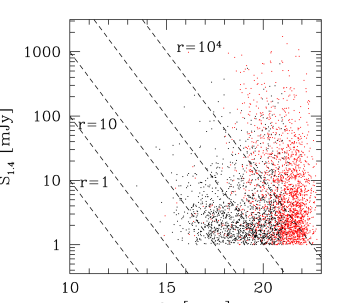
Figure 6: Radio flux S vs. $b_{J}$ magnitude. The dashed lines are the loci of constant radio-to-optical ratio r_B (see text for details). Red points indicate stellar-like sources (i.e. QSO), while the black ones are for objects identified as galaxies.

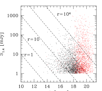
Figure 7: Radio flux S vs. R magnitude. The dashed lines are the loci of constant radio-to-optical ratio r_R (see text for details). Red points indicate stellar-like sources (i.e. QSO), while the black ones are for objects identified as galaxies.

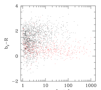
Figure 8: Colour $b_{J}-R$ vs flux for all the sources in the id-sample with $b_{J}\leq 20.5$. Red points indicate stellar-like sources (i.e. QSO), while the black ones are for objects identified as galaxies.

Figure 9: Number of sources per flux interval in the id-sample. The dotted line represents the whole sample, while the dashed and solid lines respectively are for galaxies and stellar-like sources (with $b_{J}\leq 20.5$)

The radio-to-optical ratio is defined as r_m $=\rm{S}\times 10^{({\rm m}-12.5)/2.5}$, where S is the radio flux in mJy and m is the apparent magnitude (either $R$ or $b_{J}$ depending on the specific case. We recall here that a source is considered radio-loud if r_B $\mathrel{\hbox to0.0pt{\lower 3.0pt\hbox{$\sim$}\hss}\raise 2.0pt\hbox{$>$}}10$ (see e.g. Urry & Padovani 1995). It has been shown (see for instance Magliocchetti, Celotti & Danese, 2001) that for star-bursting galaxies, where the star-formation activity is so intense that it hides the signatures of any central BH, r_B $\mathrel{\hbox to0.0pt{\lower 3.0pt\hbox{$\sim$}\hss}\raise 2.0pt\hbox{$<$}}100$. Thus the small number of sources below the r_B=100 line in Figure 6 shows that there are $<100$ star-forming galaxies in the FIRST sample down to 1 mJy. This is further confirmation of the result that star-bursting sources show up only at radio fluxes below the mJy level (see for instance, Gruppioni et al. 1998, Georgakakis et al. 1999 and MA2000).

The region of the S-$b_{J}$ plane between r $\simeq 100$ and r $\simeq 10^{4}$ is mainly dominated by sources identified as (radio) galaxies, and this population constitutes the majority of the id-sample. For r $\mathrel{\hbox to0.0pt{\lower 3.0pt\hbox{$\sim$}\hss}\raise 2.0pt\hbox{$>$}}10^{4}$ and $b_{J}\leq 20.5$ stellar identifications, most likely to be high-z QSO, dominate the sample. Fainter than $b_{J}=20.5$ this effect is mainly an artefact of the data because the optical images are too faint to resolve galaxies.

Figure 7 illustrates the flux-magnitude diagram in the $R$ band. Apart from the features already seen in Figure 6, we note an interesting shift of the population of radio galaxies towards brighter red magnitudes. This shift is especially significant for S $\mathrel{\hbox to0.0pt{\lower 3.0pt\hbox{$\sim$}\hss}\raise 2.0pt\hbox{$>$}}10$ mJy and is not observed for the stellar identifications, highlighting the fact that radio-galaxies are typically red, early-type objects.

This effect can be seen more clearly in Figure 8, which plots the $b_{J}-R$ colour of sources in the id-sample for objects with $b_{J}$ $\leq 20.5$. The majority of the id-sample consists of galaxies with very red colours, up to $b_{J}-R\sim 4$. This conclusion is actually made even stronger as in our analysis we might have missed very red sources which had $b_{J}$ magnitudes too faint to be included in the original catalogue. The id-sample was drawn from a catalogue selected on $b_{J}$ magnitude; the red magnitudes were added later as explained in Section 2. Note the clear distinction in Figure 8 between radio galaxies, which appear mostly with $b_{J}-R\mathrel{\hbox to0.0pt{\lower 3.0pt\hbox{$\sim$}\hss}\raise 2.0pt\hbox{$>$}}1$ and QSO, which dominate the region $0\mathrel{\hbox to0.0pt{\lower 3.0pt\hbox{$\sim$}\hss}\raise 2.0pt\hbox{$<$}}b_{J}-R\mathrel{\hbox to0.0pt{\lower 3.0pt\hbox{$\sim$}\hss}\raise 2.0pt\hbox{$<$}}1$. This division becomes striking for radio fluxes S $\mathrel{\hbox to0.0pt{\lower 3.0pt\hbox{$\sim$}\hss}\raise 2.0pt\hbox{$>$}}$ 10, where the two distributions take the shape of a tuning fork. Again we can see that star-forming galaxies showing blue (i.e. for $b_{J}-R\mathrel{\hbox to0.0pt{\lower 3.0pt\hbox{$\sim$}\hss}\raise 2.0pt\hbox{$<$}}0$) colours and low (S $\mathrel{\hbox to0.0pt{\lower 3.0pt\hbox{$\sim$}\hss}\raise 2.0pt\hbox{$<$}}10$) radio-fluxes constitute only a few tens of objects in the lower part of the plot.

Also when we consider the number of sources per unit of radio flux (see Figure 9) we see that stellar and non-stellar ids show different behaviours. The number of galaxies (the dashed line), shows a steeper slope than the number of QSO (the solid line). This difference reflects the fact that galaxies tend to have lower radio fluxes, while QSO dominate the region $S_{1.4{\rm GHz}}\mathrel{\hbox to0.0pt{\lower 3.0pt\hbox{$\sim$}\hss}\raise 2.0pt\hbox{$>$}}20$ mJy.

5 Spatial Distribution and Clustering Properties of the Sample

Figure 10: Projected distribution of radio sources with optical identifications: bottom panel for the whole sample ($b_{J}\leq 21.5$), middle panel for the sources identified as galaxies ($b_{J}\leq 20.5$) and top panel for those identified as stellar ($b_{J}\leq 20.5$).

The acquisition of optical identifications for radio sources is not only useful in providing optical information, it also gives the opportunity to make a distinction between low-redshift sources and more distant ones.

Passive radio galaxies are known to be reliable standard candles (see e.g. Hine & Longair, 1979; Rixon, Wall & Benn, 1991). The mean absolute magnitude in the red band is $M_{R}\simeq-23$ (see e.g. MA2000), and there is little scatter about the mean (MA2000 estimate $\Delta$M${}_{R}\simeq 0.25$ at the 1$\sigma$ level). Thus measurements of the apparent magnitude $R$ for these sources can provide us with an estimate of their redshifts according to the relation

$$R-M_{R}=-5+5{\rm log}_{10}d_{L}(pc)$$ (1)

where $d_{L}$ the luminosity distance. The id-sample is complete to $R\sim 19.5$, and from this formula we expect that objects brighter than $R\sim 19.5$ should be found in the redshift range $0\mathrel{\hbox to0.0pt{\lower 3.0pt\hbox{$\sim$}\hss}\raise 2.0pt\hbox{$<$}}z\mathrel{\hbox to0.0pt{\lower 3.0pt\hbox{$\sim$}\hss}\raise 2.0pt\hbox{$<$}}0.3$.
As we saw in the previous Section, the optically extended id-sample is mostly made up of early-type galaxies, with star-bursting objects contributing only a small fraction. So we can apply equation (1) to the whole subsample of radio galaxies, and deduce that it contains radio-sources that are mostly closer than $z\simeq 0.3$. The spread in the $R-z$ relation means that the upper redshift limit will be a gradual cutoff; see also MA2000.

The other sources that appear in the id-sample are mainly QSO with a very small contamination from nearby stars. Unfortunately, we have no simple way to distinguish between these two classes of objects, or to estimate the QSO redshift. However, apart from rare exceptions, we expect QSO to be all placed at high redshifts, at least beyond z $\mathrel{\hbox to0.0pt{\lower 3.0pt\hbox{$\sim$}\hss}\raise 2.0pt\hbox{$>$}}0.3$.
The optical distinction between point-like and extended sources as discussed in the previous Section, allows us to divide the id-sample in a low-z subsample - comprising mostly of early-type galaxies and roughly complete to $z\simeq 0.3$ - and a sample of QSO mostly found at redshifts well beyond 0.3.

Figure 10 shows the angular distribution of these sources projected on the sky. The bottom panel represents the distribution of all the objects in the id-sample with $b_{J}\leq 21.5$, limit for completeness and uniformity of the optical catalogue, while the middle one includes radio sources identified as galaxies and the top one is for point-like sources (both in the case of $b_{J}\leq 20.5$).

We can quantify the level of clustering in each sample by means of the two-point correlation function. Ideally one would like to obtain the spatial correlation function $\xi(r)$ but, since we do not have measured redshifts for any sources in the id-sample, we have to deal with its angular counterpart $w(\theta)$. We recall here that the angular two-point correlation function measures the excess probability, with respect to a random Poisson distribution, of finding two sources in the solid angles $\delta\Omega_{1}$ $\delta\Omega_{2}$ separated by an angle $\theta$. It is defined as

$$\delta P=n^{2}\delta\Omega_{1}\delta\Omega_{2}\left[1+w(\theta)\right]$$ (2)

where $n$ is the mean number density of objects in the catalogue under consideration.

We calculated $w(\theta)$ using the estimator (Hamilton, 1993)

$$w= \frac{4DD\ RR}{DR^{2}} -1,$$ (3)

where the number of data-data, random-random and data-random pairs separated by an angle $\theta$ are denoted by DD, RR and DR respectively.
Random catalogues were generated with a spatial distribution modulated by both the APM and FIRST coverage maps, so that the instrumental window functions do not affect the measured clustering. We estimate the errors on the $w(\theta)$ measurements by assuming the the pair counts follow Poisson statistics. This underestimates the uncertainties, but we do not expect this bias to be a large factor. However, the errors in $w(\theta)$ at each point are correlated, so it is easy to overestimate the significance of any features apparent in $w$.

Figure 11: The angular correlation function $1+w(\theta)$ for the whole sample of radio sources with an optical identification within $b_{J}=21.5$. Error-bars are obtained as Poissonian estimates for the catalogue under consideration. The dashed-dotted line shows the best fit to the data and is obtained for a functional form $w(\theta)=A\>\theta^{1-\gamma}$, where $A\sim 0.018$ and $\gamma\sim 1.3$.

In Figure 11 we show the results for $w(\theta)$ of the whole id-sample with $b_{J}\leq 21.5$. As already stated, error-bars are given by Poisson estimates for the catalogue under consideration. The clustering signal is significantly greater than zero at all angular scales; if we assume a power-law form for $w(\theta)$, $w(\theta)=A\>\theta^{1-\gamma}$, we find, via a $\chi^{2}$ fit to the data, $A\sim 0.018$ and $\gamma\sim 1.3$.
However, as we have already seen, the id-sample is a hybrid mixture of low- and high-z sources, which means that this measurement is not particularly relevant. More interesting information can be derived from the analysis of the clustering signal produced by the two different classes of objects, namely stellar and extended sources.

Figure 12: The angular correlation function 1+$w(\theta)$ for the subsample of radio sources (with $b_{J}\leq 20.5$) showing an optical compact structure. Error-bars are as in Figure 11.

We then estimated $w(\theta)$ for the stellar-like sources (535 objects with $b_{J}\leq 20.5$), and the resulting $1+w(\theta)$ is shown in Figure 12. The clustering signal is dominated by large errors due to the small number of objects. Nevertheless the signal is positive at almost all angular scales up to $\theta\sim 5^{\circ}$.

The most interesting result is represented by the angular correlation function for the 1494 radio galaxies in the id-sample. As illustrated by figure 13, in this case the signal is quite strong, showing once again that radio sources are more clustered than normal galaxies (see also Peacock & Nicholson, 1991; Cress et al., 1996; Loan, Wall & Lahav, 1997; Magliocchetti et al., 1998: Magliocchetti et al., 1999). In fact, if we parameterize $w(\theta)$ as a power-law: $w(\theta)=A\>\theta^{1-\gamma}$, we find - via a $\chi^{2}$ fit to the data - $A\sim 0.03$ and $\gamma\sim 2.1$, with a value for the slope close to those obtained for samples of early-type galaxies only, known to be more strongly clustered than other galaxy populations (see e.g. Maddox et al., 1990c and Loveday et al., 1995). Note that this result also agrees with the observational evidence for AGN-fuelled radio sources to be hosted by elliptical/early-type galaxies (see e.g. McLure et al., 1999).

Figure 13: The angular correlation function 1+$w(\theta)$ for the subsample of radio galaxies (with $b_{J}\leq 20.5$). Error-bars are as in Figure 11. The dashed line represents predictions from clustering evolution models (see text for details).

Since this last measurement has been obtained for a homogeneous sample of sources with a fairly well determined redshift distribution, we can predict the clustering for a range of models to be directly compared with the data. The first step in our model is to calculate the mass-mass correlation function $\xi_{m}(r,z)$. We use the analytical form derived using the Peacock & Dodds (1996) approach, extended to z $\neq 0$ by Matarrese et al. (1997). This starts with a primordial CDM power spectrum (COBE normalized in our case; Bunn & White, 1997) and writes the non-linear part of the power-spectrum $P_{NL}(k_{NL})$ as a function of its linear part $P_{L}(k_{L})$, where $k_{L}$ and $k_{NL}$ are the linear and non-linear wave-number respectively (see Magliocchetti et al. (2000a) for a complete derivation of the various quantities).

The predicted angular correlation function $w_{th}(\theta)$ can then be obtained from $\xi_{m}(r,z)$ using the relativistic Limber equation (Peebles, 1980)

$$w_{th}(\theta)=2\;\frac{\int_{0}^{z_{max}}N(z)^{2}\;\frac{dx}{dz}\;b(z)^{2}\;dz\int_{0}^{\infty}\xi_{m}(r,z)\;du}{\left[\int_{0}^{z_{max}}N(z)\;dz\right]^{2}},$$ (4)

where $x$ is the comoving coordinate, $u$ is related to the spatial distance $r$ between two sources separated by an angle $\theta$ (in the small angle approximation) via $r\simeq\left(u^{2}/F^{2}+x^{2}\theta^{2}\right)^{1/2}$ ($F$ is the curvature correction), $N(z)$ is the redshift distribution for the sources under consideration, $z_{max}$ is the maximum redshift of the sample and $b(z)$ is the bias function which determines the way radio sources trace the mass distribution. Note that, by imposing a $z_{max}$ we have assumed that the sample completeness is a step function, which immediately drops to zero beyond the redshift where the sample starts to become incomplete (0.3 in our case). We use the $N(z)$ obtained by MA2000 (Fig. 13). This is based on redshift measurements for 76 radio sources selected from both the FIRST survey and the Phoenix survey (Hopkins et al., 1998; Georgakakis et al., 1999) surveys. These samples were selected at a limit of 1 mJy and include redshift measurements up to z $\simeq 0.5$.

A little more attention has to be devoted to the issue of bias and its evolution. Of the various models presented in literature, the so-called merging model (Mo & White, 1996; Matarrese et al., 1997; Moscardini et al., 1998; Martini & Weinberg, 2001) has the most appealing physical motivation: dark matter halos simply undergo dissipative collapse (i.e. merging). However this model has been shown to not fit the clustering data at low-redshifts (see e.g. Baugh et al., 1999; Magliocchetti et al., 1999; Magliocchetti et al., 2000a to mention just a few). The reason for the discrepancy may be that the merging rate of objects is very high for z $\mathrel{\hbox to0.0pt{\lower 3.0pt\hbox{$\sim$}\hss}\raise 2.0pt\hbox{$>$}}1$ but becomes negligible for z $\mathrel{\hbox to0.0pt{\lower 3.0pt\hbox{$\sim$}\hss}\raise 2.0pt\hbox{$<$}}0.5$.
A better bias model to describe the data in this situation is the so-called galaxy conserving model (Fry, 1996). This model assumes that galaxies form at some epoch and then the clustering pattern simply evolves as the galaxies follow the continuity equation without losing their identity. It can be shown (Nusser & Davis, 1994; Fry, 1996) that bias for such galaxies evolves as

$$b(z)=1+\frac{b_{0}-1}{D(z)},$$ (5)

where $D(z)$ is the linear growth rate for clustering, and $b_{0}$ is the bias at the present epoch, $b_{0}=\sigma_{8,RG}/\sigma_{8,m}$, where $\sigma_{8}$ is the rms fluctuation amplitude in a sphere of radius 8 h^-1Mpc. We calculate $\sigma_{8,RG}$ assuming a correlation radius $r_{0}\sim 10$ h^-1Mpc for radio galaxies (Peacock & Nicholson, 1991). We calculate $\sigma_{8,m}$ using a COBE-normalized $\Lambda$CDM model with $\Omega_{0}=0.4$, $h_{0}=0.65$, $\Lambda=0.6$. The resulting prediction for $w_{th}(\theta)$ is presented in Figure 13. The match with the data is extremely good, especially when one considers that there are no free parameters in the model. This gives us confidence on our understanding of the processes regulating clustering in general and in particular the one of radio sources, at least in the nearby universe.

6 Conclusions

We have presented an analysis of the properties of optical counterparts of radio sources at the 1 mJy level. The optical identifications have been obtained by matching together objects from the FIRST and APM surveys over the region of the sky $148.13^{\circ}\mathrel{\hbox to0.0pt{\lower 3.0pt\hbox{$\sim$}\hss}\raise 2.0pt\hbox{$<$}}{\rm RA(2000)}\mathrel{\hbox to0.0pt{\lower 3.0pt\hbox{$\sim$}\hss}\raise 2.0pt\hbox{$<$}}218.13^{\circ}$, $-2.77^{\circ}\mathrel{\hbox to0.0pt{\lower 3.0pt\hbox{$\sim$}\hss}\raise 2.0pt\hbox{$<$}}{\rm Dec}\mathrel{\hbox to0.0pt{\lower 3.0pt\hbox{$\sim$}\hss}\raise 2.0pt\hbox{$<$}}2.25^{\circ}$. We found 4075 radio objects with fluxes greater than 1 mJy to be identified in the APM catalogue for $b_{J}\mathrel{\hbox to0.0pt{\lower 3.0pt\hbox{$\sim$}\hss}\raise 2.0pt\hbox{$<$}}22$ within a matching radius of 2 arcsecs (id-sample). This corresponds to 16.7 per cent of the original radio sample. A cut for $b_{J}$ = 21.5 has subsequently been applied to ensure a uniform optical sample: 3176 identifications are found brighter than this magnitude limit.

Such a wide area sample allows detailed statistical studies on the photometry of radio sources. Furthermore, with the application of the methods introduced in Maddox et al., (1990a), we managed to divide radio sources with optical identifications and $b_{J}\leq 20.5$ into radio galaxies and stellar objects (mainly QSO with some contamination from nearby stars). We find the population of radio galaxies to be almost exclusively dominated by early-type galaxies, with radio-to-optical ratios in the blue band between $10^{2}$ and $10^{4}$ and very red colours (up to $b_{J}-R\sim 4$). Starbursting objects make up only a negligible fraction of the sample. QSO tend to have $r_{B}\mathrel{\hbox to0.0pt{\lower 3.0pt\hbox{$\sim$}\hss}\raise 2.0pt\hbox{$>$}}10^{4}$ and preferentially lie in the region $0\mathrel{\hbox to0.0pt{\lower 3.0pt\hbox{$\sim$}\hss}\raise 2.0pt\hbox{$<$}}b_{J}-R\mathrel{\hbox to0.0pt{\lower 3.0pt\hbox{$\sim$}\hss}\raise 2.0pt\hbox{$<$}}1$ of the colour-radio flux diagram at all radio fluxes.

Since passive radio galaxies are known to be reliable standard candles, measurements of the apparent magnitude in the red band allowed us to divide the id-sample into two low-redshift and high-redshift catalogues, the first one - roughly complete to $z\simeq 0.3$ - made by radio galaxies and the second one including high-z QSO.

The completeness and homogeneity and defined redshift cut of the galaxy sample allowed a direct comparison between models for the angular correlation function and the data. We find an extremely good match between observational results and models if we treat radio galaxies as highly biased tracers of the underlying dark matter distribution and if we assume a bias evolution with look-back time of the form introduced by Fry (1996). This is in agreement with previous results obtained by Magliocchetti et al. (1999) for the whole sample of FIRST radio sources.

Note that, as well as the results presented in this Paper, such a large sample of radio sources with optical identifications forms an excellent basis for spectroscopic follow-up observations, which could, amongst others, fully determine the form of the redshift distribution of these objects at the mJy level out $z\mathrel{\hbox to0.0pt{\lower 3.0pt\hbox{$\sim$}\hss}\raise 2.0pt\hbox{$<$}}0.3$. We will tackle this issue in a future Paper where we will present results from the 2dF survey.

References

- [Baugh et al. 1999] Baugh C.M., Benson A.J., Cole S., Frenk C.S., Lacey C.G., 1999, MNRAS, 305, 21
- [Becker et al. 1995] Becker R.H., White R.L., Helfand D.J., 1995, ApJ, 450, 559
- [Bock et al. 1999] Bock D. C-J., Large M.I., Sadler, E.M., 1999, AJ, 117, 1578
- [Bunn and White 1997] Bunn E.F., White M., 1997, ApJ, 480, 6
- [Colless 1999] Colless M., 1999, Phil Trans R Soc Lond. A, 357, 105
- [Condon et al. 1998] Condon J.J., Cotton W.D., Greisen E.W., Yin Q.F., Perley R.A., Taylor G.B., Broderick J.J., 1998, AJ, 115, 1693
- [Cress et al. 1996] Cress C.M., Helfand D.J., Becker R.H., Gregg M.D., White R.L., 1996, ApJ, 473, 7
- [Fry 1996] Fry J.N., 1996, ApJ, 461, L65
- [Georgakakis et al. 1999] Georgakakis A., Mobasher B., Cram L., Hopkins A., Lidman C, Rowan-Robinson M., 1999, MNRAS, 306, 708
- [Gruppioni et al. 1998] Gruppioni C., Mignoli M., Zamorani G., 1998, MNRAS, 304, 199
- [Hamilton 1993] Hamilton A.J.S., 1993, ApJ, 417, 19
- [Helfand 1997] Helfand D.J. at al., 1997, AAS, 190, 4304
- [hine 1979] Hine R.G., Longair M.S., 1979, MNRAS, 188, 111
- [Hopkins et al. 1998] Hopkins A., Mobasher B., Cram L., Rowan-Robinson M. 1998, MNRAS, 296, 839
- [Loan et al. 1997] Loan A.J., Wall J.V., Lahav O., 1997, MNRAS, 286, 994
- [Loveday et al. 1995] Loveday J., Maddox S.J., Efstathiou G., Peterson B.A., 1995, ApJ, 442,457
- [Lu et al. 1996] Lu N.Y., Lyle Hoffman G.L., Salpeter E.E., Houck J.R., 1996, ApJS, 103, 331
- [Maddox et al. 1990c] Maddox S.J., Efstathiou G., Sutherland W.J., Loveday J., 1990c, MNRAS, 242, 43p
- [Maddox et al. 1990a] Maddox S.J., Efstathiou G., Sutherland W.J., Loveday J., 1990a, MNRAS, 243, 692
- [Maddox et al. 1990b] Maddox S.J., Efstathiou G., Sutherland W.J., 1990b, MNRAS, 246, 433
- [Maddox et al. 1996] Maddox S.J., Efstathiou G., Sutherland W.J., 1996, MNRAS, 283, 1227
- [Magliocchetti et al. 1998] Magliocchetti M., Maddox S.J., Lahav O., Wall J.V., 1998, MNRAS, 300, 257
- [Magliocchetti et al. 1999] Magliocchetti M., Maddox S.J., Lahav O., Wall J.V., 1999, MNRAS, 309, 943
- [Magliocchetti et al. 2000a] Magliocchetti M., Bagla J., Maddox S.J., Lahav O., 2000a, MNRAS, 314, 546
- [Magliocchetti et al. 2000] Magliocchetti M., Maddox S.J., Wall J.V., Benn C.R., Cotter G., 2000, MNRAS, 318, 1047 [MA2000]
- [Magliocchetti et al. 2001] Magliocchetti M., Celotti A., Danese L., 2001, MNRAS, submitted
- [Martini et al. 2001] Martini P., Weinberg D.H., 2001, ApJ, 547, 12
- [Masci et al. 2001] Masci F.J., Condon J.J., Barlow T.A., Lonsdale C.J., Xu C., Shupe D.L., Pevunova O., Cutri R., 2001, PASP, 113, 10
- [Matarrese et al. 1997] Matarrese S., Coles P., Lucchin F., Moscardini L., 1997, MNRAS, 286, 115
- [McLure et al. 1999] McLure R.J., Kukula M.J., Dunlop J.S., Baum S.A., O’Dea C.P., Hughes D.H., 1999, MNRAS, 308, 377
- [Mo and White 1996] Mo H., White S.D.M., 1996, MNRAS, 282, 347
- [Moscardini et al. 1998] Moscardini L., Coles P., Lucchin F., Matarrese S., 1998, MNRAS, 299, 95
- [Nusser and Davis 1994] Nusser A., Davis M., 1994, ApJ, 421, L1
- [Pea 1991] Peacock J.A., Nicholson D., 1991, MNRAS, 253, 307
- [Peacock2 1996] Peacock J.A., Dodds S.J., 1996, MNRAS, 267, 1020
- [Peebles 1980] Peebles P.J.E., 1980, The Large-Scale Structure of the Universe, Princeton University Press
- [Rixon et al. 1997] Rixon G.T., Wall J.V., Benn C.R., 1991, MNRAS, 251, 243
- [Sadler et al. 1999] Sadler E.M., McIntyre V.J., Jackson C.A., Cannon R.D., 1999, PASA, 16, 247
- [Urry 1995] Urry C.M., Padovani P., 1995, PASP, 107, 803
- [White et al. 1997] White R.L., Becker R.H., Helfand D.J., Gregg M.D., 1997, ApJ, 475, 479