The Fate of an Accelerating Universe

The presently accelerating universe may keep accelerating forever, eventually run into the event horizon problem, and thus be in conflict with the superstring idea. In the other way around, the current accelerating phase as well as the fate of the universe may be swayed by a negative cosmological constant, which dictates a big crunch. Based on the current observational data, in this paper we investigate how large the magnitude of a negative cosmological constant is allowed to be. In addition, for distinguishing the sign of the cosmological constant via observations, we point out that a measure of the evolution of the dark energy equation of state may be a good discriminator. Hopefully future observations will provide much more detailed information about dark energy and thereby indicates the sign of the cosmological constant as well as the fate of the presently accelerating universe.

1 Introduction

The accelerating expansion of the present universe was suggested by the type Ia supernova (SN Ia) distance measurements [1, 2] in 1998 and reinforced recently by updated SN Ia data [3, 4, 5, 6] and WMAP measurement [7] of cosmic microwave background (CMB). One general conclusion from these measurements and other CMB observations in recent years [8, 9, 10] is that the universe has the critical density, consisting of $27\%$ pressureless matter and $73\%$ dark energy with a negative pressure [11] (such that $p/\rho<-0.78$ [7]).

The most promising candidates to account for dark energy include (i) a cosmological constant [12], (ii) a slowly evolving scalar field called “quintessence” [13], (iii) the presence of extra dimensions on top of the well-known $3+1$ space-time [14, 15, 16, 17], and (iv) the modification of gravity [18, 19, 20]. The existence of a positive cosmological constant is the simplest candidate for dark energy. The cosmological constant may be provided by various kinds of matter/energy, such as the vacuum energy of quantum fields and the potential energy of classical fields, and could also be originated in the intrinsic geometry. Nevertheless, Shapiro and Sola [21] show that the scaling behavior of such cosmological constant, when embedded in the framework of the standard model of elementary particle physics, inevitably leads to a cosmological constant of right size but opposite in sign. As to other dark energy candidates, quintessence is usually realized by a slowly evolving mode (or coherent state) of a real scalar field while the possibility of realizing quintessence by a complex scalar field was also pointed out in [22, 23]. Quintessence provides dynamical negative pressure and could in principle avoid the fine tuning problem. For example, the“tracker fields” proposed by Zlatev et al. entail solutions which will join a common cosmic evolutionary path, regardless of a wide range of initial conditions [24]. We shall leave the discussions on the possibility of understanding the accelerating universe via extra dimensions to other papers of ours [15, 17].

Another general consensus is that the present universe is thus already dominated by dark energy and, in light of general relativity and cosmological principle, there is no way to overrun the dominance of dark energy over the other familiar form of matter or energy. It is therefore of fundamental interest to examine the possibilities resulting an eternally accelerating universe [25, 26, 27, 28]. If the expansion of the universe keeps accelerating forever, the universe will have to exhibit an event horizon, raising the issue about the viability of the current description of string theory: The existence of the event horizon brings challenges to string theory, such as the construction of suitable observables to displace the problematic conventional S-matrix in the universe with an event horizon [25, 26, 29].

However, there is a pitfall in the chain of the arguments leading to an eternally accelerating universe. That is, there might be competitive components in our universe and at present only one such form, say quintessence of some kind, has assumed its control. For example, it is perfectly justified to assume that a negative cosmological constant, whose existence may be a natural occurrence as suggested in [21, 30, 31, 32], could be present but yet to exert its control in the distant future. The existence of a negative cosmological constant is more compatible with string theory [29]. The possibility of an accelerating universe with a negative cosmological constant has been considered in [30, 33, 34] for the renormalization-group running of the cosmological constant (vacuum energy) and in [35, 36, 37] for quintessence.

Thus, after introducing the basics in cosmology in the next section, we study several simple examples in Sec. 3 for demonstrating various possible fates of the presently accelerating universe which are swayed by a cosmological constant, in particular, its sign. In Sec. 4 we investigate how negative, confronting the constraints from various astronomical observations, a cosmological constant is allowed to be, and propose a phenomenological discriminator of the sign of the cosmological constant. A summary follows in Sec. 5.

2 Basics

In standard cosmology, the universe at large scales is described by the Friedmann-Robertson-Walker (FRW) metric,

$$ds^{2}=dt^{2}-a^{2}(t)\left(\frac{dr^{2}}{1-kr^{2}}+r^{2}d\Omega^{2}\right),$$ (1)

which respects from the cosmological principle, i.e., homogeneity and isotropy. In Eq. (1), $a(t)$ is the (cosmic) scale factor, and $k$ can be chosen to be $+1$, $-1$, or $0$, corresponding to a closed, open, or flat universe, respectively. Provided that the matter content of the universe is taken to be a perfect fluid, the Einstein equations yield

$$\left(\frac{\dot{a}}{a}\right)^{2}+\frac{k}{a^{2}}=\frac{8\pi G}{3}\tilde{\rho}=\frac{\Lambda}{3}+\frac{8\pi G}{3}\rho\;,$$ (2)

$$\frac{\ddot{a}}{a}=-\frac{4\pi G}{3}(\tilde{\rho}+3\tilde{p})=\frac{\Lambda}{3}-\frac{4\pi G}{3}(\rho+3p)\;,$$ (3)

and also imply the energy-momentum conservation,

$$d(\tilde{\rho}a^{3})=-\tilde{p}d(a^{3})\;,$$ (4)

where $\tilde{\rho}$ and $\tilde{p}$ are effective energy density and pressure of the perfect fluid including the contributions from a cosmological constant $\Lambda$ and other matter contents. As indicated in Eq. (3), the expansion of the universe is accelerating if the pressure $\tilde{p}$ is so negative that

$$\tilde{p}<-\frac{1}{3}\tilde{\rho}<0\;,\quad\mbox{provided }\tilde{\rho}>0\;.$$ (5)

The universe is usually considered to be composed of various kinds of perfect fluids with different types of equations of state:

$$p_{i}=w_{i}\rho_{i}\;,$$ (6)

where $\rho_{i}$ and $p_{i}$ are energy density and pressure of the $i$-th component, and the equation-of-state factor $w_{i}$ in general may depend on energy density $\rho_{i}$ and time. Assuming that each (fluid) component evolves independently and each $w_{i}$ is constant, we obtain, from Eq. (4), a relation between the energy density $\rho_{i}$ and the scale factor $a(t)$:

$$\rho_{i}\propto a^{-3(1+w_{i})}\,.$$ (7)

This relation implies that the energy density of the component with a smaller equation-of-state factor $w$ drops more slowly along with the expansion of the universe. As a result, eventually the universe will be dominated by the component with the smallest equation-of-state factor $w$ as long as the universe keeps expanding at all times.

3 Examples

As one prominent candidate of dark energy, quintessence may play a crucial role in swaying the fate of the universe. In addition, the cosmological constant, which entails the smallest equation-of-state factor ($w=-1$) among “non-phantom” ($w\geq-1$) dark energy sources, may take over to dominate the universe eventually. Therefore, in this section we will explore how these two kinds of energy sources will affect the ultimate fate of the presently accelerating universe.

Quintessence

We consider a Lagrangian density of a scalar field for the quintessence as follows:

$$\mathcal{L}=\sqrt{|g|}\left[\frac{1}{2}g^{\mu\nu}(\partial_{\mu}\phi)(\partial_{\nu}\phi)-V(\phi)\right].$$ (8)

For simplicity, here we consider a universe which at large scales is homogeneous, isotropic, and spatially flat, and accordingly can be described by the flat FRW metric ($k=0$) in Eq. (1). Although we focus on this highly symmetric space at large scales, the small-scale behavior of the field $\phi$ in general does make contributions to the stress energy of $\phi$, and accordingly is involved in the calculation of the energy-momentum tensor. More precisely, when we invoke the cosmological principle and the Einstein equations of large scales (corresponding to the FRW metric), the energy-momentum tensor contributed by a field is the spatially averaged stress energy of the field (to which the small-scale spatial variations do make contributions), but not the stress energy of the spatially averaged field. Thus, regarding the calculation of the large-scale energy-momentum tensor contributed by a field, in general we should take the possible small-scale variations of the field into consideration, instead of ignoring them simply through the requirement of homogeneity and isotropy of the universe at large scales. However, in order for the quintessence field $\phi$ to generate accelerating expansion, the weak spatial dependence of the field is requisite, as to be explained in the following.

To describe the small-scale behavior and to calculate the stress energy of a field, in general we should consider a more general metric instead of the FRW metric. Here, for simplicity, we assume that the deviation from the background FRW metric is insignificant, and accordingly we ignore the metric perturbations. In this case the field equation of the scalar field $\phi$ is

$$\frac{\partial^{2}\phi}{\partial t^{2}}+3H\frac{\partial\phi}{\partial t}-\frac{1}{a^{2}}\nabla^{2}\phi+V^{\prime}(\phi)=0\;,$$ (9)

and the energy density and pressure of the quintessence are given by

$$\rho_{\textsc{q}} = \frac{1}{2}\left(\frac{\partial\phi}{\partial t}\right)^{2}+\frac{1}{2a^{2}}\left(\nabla\phi\right)^{2}+V(\phi)\;,$$ (10)

$$p_{\textsc{q}} = \frac{1}{2}\left(\frac{\partial\phi}{\partial t}\right)^{2}-\frac{1}{6a^{2}}\left(\nabla\phi\right)^{2}-V(\phi)\;.$$ (11)

In Eq. (9), the Hubble expansion rate $H$ is defined as $H\equiv\dot{a}/a$, and $3H(\partial\phi/\partial t)$ can be regarded as a damping term caused by the expansion of the universe. Eqs. (10) and (11) imply that the equation-of-state factor $w_{\textsc{q}}$ (i.e. $p_{\textsc{q}}/\rho_{\textsc{q}}$) of the quintessence ranges from $-1$ to $1$. As mentioned above, in the Einstein equations corresponding to the FRW metric which describes the universe at large scales, the energy-momentum tensor involves the spatial average of the above energy density and pressure. These spatially averaged (over large enough scales) quantities should be independent of the spatial coordinates for the requirement of homogeneity and isotropy. Furthermore, as indicated by Eqs. (9)–(11), the spatial variation of $\phi$ (that provides vanishing $\rho_{\textsc{q}}+3p_{\textsc{q}}$) in general can induce the time variation of $\phi$ that provides positive pressure. Thus, in order to generate negative enough pressure and the accelerating expansion, both the weak spatial dependence and the slow evolution of the quintessence field $\phi$ are requisite.

As summarized in [25, 26], there are various kinds of quintessence models leading to a perpetually accelerating universe and accordingly exhibiting an event horizon. For example, for the potential proposed by Ratra and Peebles,

$$V(\phi)\sim\exp\left(-\sqrt{\frac{3}{2}(\kappa+1)}\phi\right),$$ (12)

with $\kappa<-1/3$, we have solutions which will approach to the equation of state $p=\kappa\rho$ eventually [38]. Consequently this class of potentials with $\kappa<-1/3$ will generate a perpetually accelerating universe. In addition, for the potential (originally studied in [38])

$$V(\phi)=\frac{M^{4+n}}{\phi^{n}}\,,$$ (13)

we have “tracker solutions” which approach to an equation of state $p=-\rho$ asymptotically, insuring the eternal acceleration [24]. The potential in Eq. (13) can be classified to a wider class of potentials referred to as “runaway scalar fields”, in which $V$, $V^{\prime}$, $V^{\prime\prime}$, $V^{\prime}/V$, and $V^{\prime\prime}/V$ all approach $0$ as $\phi\rightarrow\infty$ [39]. Steinhardt claimed that the runaway scalar field will guarantee the eventual acceleration of the universe. Nevertheless, there are other possible quintessence models providing alternative results [26, 40, 41]. For example, for a potential which drops to a minimum at $\phi_{0}$ and then becomes flat for $\phi>\phi_{0}$, the universe will be dominated by the kinetic energy after the scalar field passes the minimum, and then become decelerating with an equation of state $p=\rho$.

There are two more points which should be added. Firstly, the existence of a nonzero minimum of the quintessence potential bounded by below can make a contribution to the cosmological constant. We will categorize the possibly nonzero minimum of the potential as a part of the cosmological constant, and accordingly set this minimum to be zero after introducing the cosmological constant. Secondly, we note that the kinetic energy and potential energy of the quintessence are transferred to each other along with the evolution of the quintessence field. In addition, the kinetic energy is dissipated, accompanying the expansion of the universe, due to the damping term $3H(\partial\phi/\partial t)$ in Eq. (9). As a result, in general the energy density of the quintessence will be dissipated as the universe expands, and the equation-of-state factor $w_{\textsc{q}}$ can only skim over or approach $-1$ (rather than halting at that point) and hence should be always larger than that of a cosmological constant.

The Cosmological Constant

Provided that there is no “phantom” energy with the equation of state $w<-1$ [42, 43], the cosmological constant, with the smallest equation-of-state factor ($w=-1$), will eventually dominate the universe as long as the universe keeps on expanding at all times. In the following, using Eqs. (2) and (3), we will see how a positive and a negative cosmological constant will affect the fate of the universe profoundly in totally different ways.

(i) $\Lambda>0$

In both the open ($k=-1$) and the flat ($k=0$) case, the universe will expand forever, and the cosmological constant will take over eventually such that the expansion will eternally accelerate thereafter, consequently exhibiting an event horizon. For a closed ($k=1$) universe, the situation is more complicated. It involves a competition between three terms in the Friedmann equation (2): the curvature term $k/a^{2}$, the cosmological constant term $\Lambda/3$, and the energy density term $\frac{8\pi G}{3}\rho$ from the matter contents other than the cosmological constant. Roughly speaking, if the cosmological constant has already become predominant before the moment when the curvature term is comparable to the matter density term, the universe will then expand forever in an accelerating manner and exhibit an event horizon. Conversely, if the cosmological constant is still comparatively small at that moment, the universe will collapse eventually (a big crunch).

(ii) $\Lambda<0$

In the case of the negative cosmological constant the universe will always collapse eventually [44] (see also [45]). We can see, from Eq. (2), that the universe will start to collapse at the moment when

$$\frac{k}{a^{2}}=\frac{\Lambda}{3}+\frac{8\pi G}{3}\rho\;,$$ (14)

no matter the universe is open, flat, or closed and how close to zero the negative cosmological constant might be.

For a concrete demonstration, we analyze numerically the evolution of the universe which is composed of a negative cosmological constant (with energy density $\rho_{\scriptscriptstyle\Lambda}$) and a quintessence field $\phi$ with the potential

$$V(\phi)=\frac{M^{6}}{\phi^{2}}\;.$$ (15)

We use the unit system in which $c=8\pi G/3=H_{0}=1$ (where $H_{0}$ is the present Hubble expansion rate). With this unit system, the constant $M$ in Eq. (15) is chosen to be unity, i.e., $M=(3H_{0}/8\pi G)^{1/3}c=1$. The results are presented in Figs. 1 and 2. These two figures sketch the evolution of the scale factor $a(t)$ and the Hubble expansion rate $H(t)\equiv\dot{a}/a$ of two universes, where the time $t$ is in unit of the present Hubble time $H_{0}^{-1}$ and $t=0$ denotes the present time. The solid line is for the case of $\rho_{\scriptscriptstyle\Lambda}=-\frac{1}{50}\rho_{\textsc{q}}(0)$, where $\rho_{\textsc{q}}(0)$ is the present energy density of the quintessence, and the dash line sketches an accelerating, nearly exponential expansion of the universe in the case of $\rho_{\scriptscriptstyle\Lambda}=0$ as a reference. As shown in these two figures, the universe with a negative cosmological constant will collapse (i.e. $\ln[a(t)/a_{0}]$ drops and $H(t)$ becomes negative) eventually, in contrast to the case of $\rho_{\scriptscriptstyle\Lambda}=0$, even though the energy density from the cosmological constant only accounts for 2 percent of that from the quintessence initially.

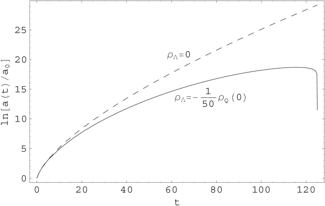
Figure 1: The plot of $ln[a(t)/a_{0}]$, describing the evolution of the universe with $\rho_{\scriptscriptstyle\Lambda}=-\frac{1}{50}\rho_{\textsc{q}}(0)$ and $\rho_{\scriptscriptstyle\Lambda}=0$, respectively. The time $t$ is in unit of the Hubble time $H_{0}^{-1}$ and $t=0$ denotes the present time.

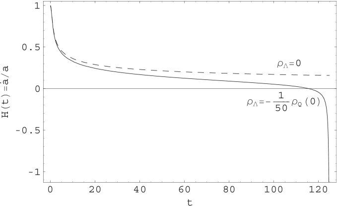
Figure 2: The plot of $H(t)$, describing the evolution of the universes with $\rho_{\scriptscriptstyle\Lambda}=-\frac{1}{50}\rho_{\textsc{q}}(0)$ and $\rho_{\scriptscriptstyle\Lambda}=0$, respectively. The time $t$ is in unit of the Hubble time $H_{0}^{-1}$ and $t=0$ denotes the present time.

We note that the collapse takes place and proceeds in a violent manner since the original “damping” term $3H(\partial\phi/\partial t)$ in Eq. (9) turns to an “amplifying” term when the universe is collapsing, i.e., $H<0$. In this collapsing epoch, the kinetic energy $\frac{1}{2}(\partial\phi/\partial t)^{2}$ of the quintessence becomes more and more dominant due to this amplifying effect. After the universe is dominated by the kinetic energy, it takes a finite time comparable to or even shorter than the present Hubble time $H_{0}^{-1}$ for the universe to collapse to the singularity. This can be shown by the following formulae for a quintessential-kinetic-energy-dominated collapsing universe:

$$\left|H\right| \simeq \sqrt{\frac{8\pi G}{3}\rho_{\textsc{q}}}\simeq\sqrt{\frac{4\pi G}{3}\left(\frac{\partial\phi}{\partial t}\right)^{2}}$$ (16)

$$> \sqrt{\frac{8\pi G}{3}\left|\rho_{\scriptscriptstyle\Lambda}\right|}\simeq H_{0}/\sqrt{50}\;,$$

$$\left|H\right| \simeq \frac{1}{3(A-t)}\quad\quad\mbox{($A$ : a constant)}\,.$$ (17)

Equation (17) is straightforwardly obtained by solving Eqs. (2) and (9) with the assumption of the dominance of the kinetic energy.

The above studies reveal a fact that the ultimate fate of the universe is determined by the cosmological constant (if there is no “phantom” energy). In particular, the future evolution pattern of our presently accelerating universe under the control of quintessence can be totally changed by the presence of a negative cosmological constant, which is part of the dark energy but may be yet too small to be detected. Consequently, it is impossible to predict the ultimate fate of our universe without knowing the detailed nature of the dark energy content therein.

In the following section we shall explore the possibility of the existence of a negative cosmological constant, confronting the constraints obtained from various astronomical observations. We shall see that the negative cosmological constant may not be tiny; instead, a model with a significant, negative cosmological constant is consistent with the current observational data.

4 Phenomenology

For simplicity, we consider a flat universe dominated by three components: (i) non-relativistic matter, including (cold) dark matter, with $\Omega_{m}\cong 0.27$ [46], (ii) a cosmological constant $\Lambda$, and (iii) a smoothly distributed energy source X that possesses positive energy density and a constant, negative equation-of-state factor $w_{\textsc{x}}$ and is responsible for the present accelerating expansion. For X to be different from a cosmological constant, we require $w_{\textsc{x}}\neq-1$. In this model, dark energy consists of two components, $\Lambda$ and X; its energy density, pressure, and the equation-of-state factor are as follows: $\rho_{\textsc{de}}=\rho_{\textsc{x}}+\rho_{\scriptscriptstyle\Lambda}$, $p_{\textsc{de}}=p_{\textsc{x}}+p_{\scriptscriptstyle\Lambda}$, and

$$w_{\textsc{de}}=\frac{p_{\textsc{x}}+p_{\scriptscriptstyle\Lambda}}{\rho_{\textsc{x}}+\rho_{\scriptscriptstyle\Lambda}}=\frac{w_{\textsc{x}}\rho_{\textsc{x}}-\rho_{\scriptscriptstyle\Lambda}}{\rho_{\textsc{x}}+\rho_{\scriptscriptstyle\Lambda}}\,.$$ (18)

In this model there are two free parameters: $w_{\textsc{x}}$ and $\Omega_{\scriptscriptstyle\Lambda}$ (or $\rho_{\scriptscriptstyle\Lambda}$). We can obtain information about these two parameters by invoking the constraints from observations on various physical quantities. In the following, we shall invoke the constraints obtained by Wang and Tegmark in [47], using SN Ia (in particular, the “gold” set [6]), CMB [9, 10, 7], and galaxy clustering [48] data. These constraints are respectively on the dark energy density $\rho_{\textsc{de}}$ as a function of redshift $z$ and on the parameters $w_{\textsc{de}}(0)$ and $w^{\prime}_{\textsc{de}}(0)$, where ‘0’ denotes the present time (i.e., $z=0$), and $w^{\prime}_{\textsc{de}}(0)\equiv dw_{\textsc{de}}/dz\,(z=0)$.

Introducing $\xi\equiv\rho_{\scriptscriptstyle\Lambda}(0)/\rho_{\textsc{x}}(0)=\Omega_{\scriptscriptstyle\Lambda}/\Omega_{\textsc{x}}$, we write the formulae for $\rho_{\textsc{de}}(z)$, $w_{\textsc{de}}$ and $w^{\prime}_{\textsc{de}}(0)$ as follows:

$$\frac{\rho_{\textsc{de}}(z)}{\rho_{\textsc{de}}(0)} = \frac{(1+z)^{3(1+w_{\textsc{x}})}+\xi}{1+\xi}\,,$$ (19)

$$w_{\textsc{de}}\hskip 5.0pt = \frac{w_{\textsc{x}}(1+z)^{3(1+w_{\textsc{x}})}-\xi}{(1+z)^{3(1+w_{\textsc{x}})}+\xi}\,,$$ (20)

$$1+w_{\textsc{de}}(0) = \frac{1+w_{\textsc{x}}}{1+\xi}\,,$$ (21)

$$w^{\prime}_{\textsc{de}}(0) = \frac{3(1+w_{\textsc{x}})^{2}\xi}{(1+\xi)^{2}}=3\left[1+w_{\textsc{de}}(0)\right]^{2}\xi\,.$$ (22)

We require $\xi>-1$ for insuring that the dark energy density is positive. According to Eq. (21), if $\xi>-1$, $w_{\textsc{de}}(0)$ and $w_{\textsc{x}}$ are simultaneously larger or smaller than $-1$. Accordingly the sign of $1+w_{\textsc{de}}(0)$ can tell us whether the dark energy component X is “phantom” ($w_{\textsc{x}}<-1$) or not. In addition, as shown in Eq. (22), the sign of $w^{\prime}_{\textsc{de}}(0)$, i.e., whether the equation-of-state factor of dark energy is increasing or decreasing, is determined by the sign of the cosmological constant. As a result, in our model the sign of $w^{\prime}_{\textsc{de}}(0)$ can be a discriminator of the sign of the cosmological constant phenomenologically. In particular, currently increasing (i.e., decreasing with $z$) $w_{\textsc{de}}$ indicates the existence of a negative cosmological constant.

In Fig. 3, we demonstrate how well this model with a negative cosmological constant satisfies the constraint on the evolution of the dark energy density. The grey region shows the $1\sigma$ constraint on $\rho_{\textsc{de}}(z)$, which is obtained in [47] by using the parametrization of the 3-parameter spline. The solid curves present the behavior of $\rho_{\textsc{de}}(z)$ predicted in models with various values of $w_{\textsc{x}}$ and $\xi$ which satisfy the $1\sigma$ constraint. These plots show that the existence of a significant, negative cosmological constant is allowed. For example, for the case $w_{\textsc{x}}=-0.9$, $-\xi$ is allowed to be as large as $0.6$, that is, at present the magnitude of the energy density of the cosmological constant is allowed to be larger than one half of that of the dark energy component X, and accordingly is larger than the dark energy density.

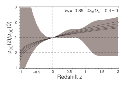
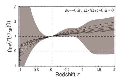
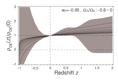
Figure 3: The $1\sigma$ constraint on $\rho_{\textsc{de}}(z)$ (presented by the grey region) and the predictions in various theoretical models which satisfy this constraint (presented by solid curves).

In Figs. 4 and 5, we demonstrate how well this model with a negative cosmological constant satisfies the constraint on $w_{\textsc{de}}(0)$ and $w^{\prime}_{\textsc{de}}(0)$. The grey region is ruled out by SN Ia data, with the prior $\Omega_{m}=0.27\pm 0.04$, at 95% confidence [47]. In Fig. 4, the black area represents the models with the parameters in the range $\left\{-1.2<w_{\textsc{x}}<-0.65\,,\,\xi>-0.5\right\}$, which are within the allowed (white) region. We note that $\xi=-0.5$ corresponds to $|\Omega_{\scriptscriptstyle\Lambda}|=\Omega_{\textsc{de}}=\Omega_{\textsc{x}}/2$ and therefore indicates a significant, negative cosmological constant. For more details, in Fig. 5 we illustrate the allowed range of $\xi$ for various values of $w_{\textsc{x}}$. From the left to the right side, the solid curves correspond to theoretical models $\{w_{\textsc{x}}\,,\,\xi>\xi_{m}\}$ with different values of $w_{\textsc{x}}$ and $\xi_{m}$, as listed in the following:

$w_{\textsc{x}}$	$-1.4$	$-1.3$	$-1.2$	$-1.1$	$-1.01$	$-0.99$	$-0.9$	$-0.8$	$-0.7$	$-0.6$
$\xi_{m}$	$-0.12$	$-0.3$	$-0.5$	$-0.74$	$-0.97$	$-0.99$	$-0.9$	$-0.8$	$-0.6$	$-0.3$

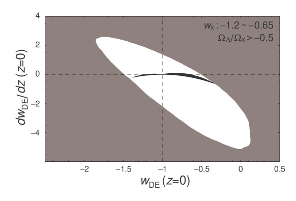
Figure 4: The constraint on $w_{\textsc{de}}(0)$ and $w^{\prime}_{\textsc{de}}(0)$ (presented by the white region) and the predictions in various theoretical models: $-1.2<w_{\textsc{x}}<-0.65$ and $\xi\equiv\Omega_{\scriptscriptstyle\Lambda}/\Omega_{\textsc{x}}>-0.5$ (presented by the black area), which survive this constraint. The grey region is ruled out by SN Ia data, with the prior $\Omega_{m}=0.27\pm 0.04$, at $95\%$ confidence.

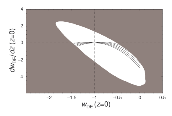
Figure 5: The constraint on $w_{\textsc{de}}(0)$ and $w^{\prime}_{\textsc{de}}(0)$ (presented by the white region) and the predictions in various theoretical models which survive this constraint. The grey region is ruled out by SN Ia data, with the prior $\Omega_{m}=0.27\pm 0.04$, at $95\%$ confidence. The solid curves, from the left to the right side, correspond to theoretical models $\{w_{\textsc{x}}\,,\,\xi>\xi_{m}\}$ with $(w_{\textsc{x}}\,,\,\xi_{m})$ = $(-1.4\,,-0.12)$ , $(-1.3\,,-0.3)$ , $(-1.2\,,-0.5)$ , $(-1.1\,,-0.74)$ , $(-1.01\,,-0.97)$ , $(-0.99\,,-0.99)$ , $(-0.9\,,-0.9)$ , $(-0.8\,,-0.8)$ , $(-0.7\,,-0.6)$ , $(-0.6\,,-0.3)$.

These plots show that, confronting the current constraints from observations, the existence of a significant, negative cosmological constant is allowed. For example, $-\xi$ is allowed to be as large as 0.9 for the case $w_{\textsc{x}}=-0.9$, and 0.5 for $w_{\textsc{x}}=-1.2$. Even for the case $w_{\textsc{x}}=-0.6$ that is not consistent with the $1\sigma$ constraint in Fig. 3, $-\xi$ is still allowed to as large as $0.3$. Thus, the existence of a negative cosmological constant is fairly consistent with the current observational data. For the case $w_{\textsc{x}}>-1$, the existence of a negative cosmological constant dictates a big crunch as the fate of the presently accelerating universe, while a positive cosmological constant dictates eternal acceleration. For $w_{\textsc{x}}<-1$, the “phantom” dark energy component X dictates a singular fate in a finite time, so-called “Big Rip” (i.e., with the scale factor $a$ blowing up), before which the expansion of the universe keeps accelerating [42, 43].

As mentioned above, in this simple model where the dark energy component X possesses a constant equation-of-state factor $w_{\textsc{x}}$, the signs of $1+w_{\textsc{de}}(0)$ and $w^{\prime}_{\textsc{de}}(0)$ (which hopefully can be obtained from future observations) respectively can tell us the signs of $1+w_{\textsc{x}}$ and $\xi$, i.e., whether the dark energy component X is “phantom” or not and whether the cosmological constant is positive or negative. This feature and the relation between the fate of the presently accelerating universe and the parameters $w_{\textsc{x}}$ and $\xi$ are summarized in the following table.

$w_{\textsc{de}}(0)$ and $w_{\textsc{x}}$	$w^{\prime}_{\textsc{de}}(0)$ and $\Lambda$	Fate
$>-1$	$+$	accelerating forever
$>-1$	$-$	Big Crunch
$<-1$	$+$	accelerating until Big Rip
$<-1$	$-$	accelerating until Big Rip

For a more general model where $w_{\textsc{x}}(z)$ is not a constant, the generalized version of Eqs. (21) and (22) is as follows:

$$1+w_{\textsc{de}}(0) = \frac{1+w_{\textsc{x}}(0)}{1+\xi}\,,$$ (23)

$$w^{\prime}_{\textsc{de}}(0) = \frac{w^{\prime}_{\textsc{x}}(0)}{1+\xi}+\frac{3\left[1+w_{\textsc{x}}(0)\right]^{2}\xi}{(1+\xi)^{2}}$$ (24)

$$= \frac{w^{\prime}_{\textsc{x}}(0)}{1+\xi}+3\left[1+w_{\textsc{de}}(0)\right]^{2}\xi\,.$$

In this case, the information about the sign of $1+w_{\textsc{de}}(0)$ obtained from observations can still tell us whether the dark energy component X is “phantom” or not. As to the sign of the cosmological constant, the situation is more complicated. If $w_{\textsc{x}}(z)$ is an arbitrary function, there is no hope to extract information about $\xi$ or $\rho_{\scriptscriptstyle\Lambda}$ because phenomenologically it is redundant to introduce a cosmological constant in this case. Nevertheless, for each category of theoretical models where $w_{\textsc{x}}(z)$ is further specified by some theoretical requirements, obtaining information about the cosmological constant from observations is feasible in principle. For example, for theoretical models where $w_{\textsc{x}}(z)$ is determined by $n$ parameters, the information about the cosmological constant can be extracted from the observational constraints on $w_{\textsc{x}}(0)$, $w^{\prime}_{\textsc{x}}(0)$, $w^{\prime\prime}_{\textsc{x}}(0)$, $\ldots$ , $w^{(n)}_{\textsc{x}}(0)$ where the superscript ‘$(n)$’ denotes the $n$-th derivative of $w_{\textsc{x}}$ with respect to redshift $z$. In particular, for models where $w_{\textsc{x}}$ at the present epoch is barely dynamical and satisfies $w^{\prime}_{\textsc{x}}(0)\ll 3\left[w_{\textsc{x}}(0)+1\right]^{2}$, the sign of $w^{\prime}_{\textsc{de}}$ can still reflect the sign of the cosmological constant in the same way as that in the case of constant $w_{\textsc{x}}$.

5 Summary

To sum up, we have demonstrated, through simple examples, how the current accelerating phase as well as the fate of the universe can be swayed by a negative cosmological constant. A negative cosmological constant may in fact be a natural occurrence, as suggested in [21, 30, 31, 32]. We have shown that the existence of a significant, negative cosmological constant is consistent with the current observational data, if the present accelerating expansion is generated by another dark energy component. As a result, the present accelerating situation does not guarantee the existence of an event horizon in conflict with the current description of string theory.

We have pointed out that phenomenologically a measure of the dynamical behavior of the equation-of-state factor of dark energy ($w_{\textsc{de}}$) may be a good discriminator of the sign of the cosmological constant: positive (negative) $dw_{\textsc{de}}/dz\,(0)$ corresponds to a positive (negative) cosmological constant. In addition, the measure of the sign of $1+w_{\textsc{de}}(0)$ can tell us whether the dark energy component (if exists) other than a cosmological constant is “phantom” or not. These two discriminators work in the cases where the equation-of-state factor of the dark energy component X barely changes with time and the cosmological constant is exactly a constant. In some other cases they may not work. For example, in the dark-energy model invoking the renormalization-group running of the cosmological constant [21, 49, 50], the variable cosmological constant with $w=-1$ can effectively behave as normal quintessence ($w>-1$) or phantom dark energy ($w<-1$) in different situations [51, 52], and therefore does not fit the above requirements for the validity of these discriminators.

So far the observational data are not good enough to tell us the tendency of the evolution of the dark energy equation of state. Accordingly both the case of a positive cosmological constant (alone) and the case of a negative cosmological constant (together with another dark energy component which provides anti-gravity and generates the present accelerating expansion) are consistent with the current data. Hopefully future data (e.g., data from Supernova Acceleration Probe (SNAP) [53] and Joint Efficient Dark-energy Investigation (JEDI) [54]) will provide much more detailed information about the evolution of the dark energy equation of state, and thereby indicate the sign of the cosmological constant and the fate of the presently accelerating universe.

References

- [1] S. Perlmutter et al. [Supernova Cosmology Project Collaboration], Astrophys. J. 517, 565 (1999) [arXiv:astro-ph/9812133].
- [2] A. G. Riess et al. [Supernova Search Team Collaboration], Astron. J. 116, 1009 (1998) [arXiv:astro-ph/9805201].
- [3] J. L. Tonry et al. [Supernova Search Team Collaboration], Astrophys. J. 594, 1 (2003) [arXiv:astro-ph/0305008].
- [4] R. A. Knop et al. [The Supernova Cosmology Project Collaboration], Astrophys. J. 598, 102 (2003) [arXiv:astro-ph/0309368].
- [5] B. J. Barris et al., Astrophys. J. 602, 571 (2004) [arXiv:astro-ph/0310843].
- [6] A. G. Riess et al. [Supernova Search Team Collaboration], Astrophys. J. 607, 665 (2004) [arXiv:astro-ph/0402512].
- [7] C. L. Bennett et al., Astrophys. J. Suppl. 148, 1 (2003) [arXiv:astro-ph/0302207]; D. N. Spergel et al. [WMAP Collaboration], Astrophys. J. Suppl. 148, 175 (2003) [arXiv:astro-ph/0302209].
- [8] J. L. Sievers et al., Astrophys. J. 591, 599 (2003) [arXiv:astro-ph/0205387].
- [9] T. J. Pearson et al., Astrophys. J. 591, 556 (2003) [arXiv:astro-ph/0205388].
- [10] C. L. Kuo et al. [ACBAR collaboration], Astrophys. J. 600, 32 (2004) [arXiv:astro-ph/0212289].
- [11] A. Balbi et al., Astrophys. J. 545, L1 (2000) [arXiv:astro-ph/0005124]; P. de Bernardis et al. [Boomerang Collaboration], in Proceedings of the CAPP2000 conference [arXiv:astro-ph/0011469].
- [12] L. M. Krauss and M. S. Turner, Gen. Rel. Grav. 27, 1137 (1995) [arXiv:astro-ph/9504003]; J. P. Ostriker and P. J. Steinhardt, Nature 377, 600 (1995); A. R. Liddle, D. H. Lyth, P. T. Viana and M. White, Mon. Not. Roy. Astron. Soc. 282, 281 (1996) [arXiv:astro-ph/9512102].
- [13] R. R. Caldwell, R. Dave and P. J. Steinhardt, Phys. Rev. Lett. 80, 1582 (1998) [arXiv:astro-ph/9708069].
- [14] C. Deffayet, G. R. Dvali and G. Gabadadze, Phys. Rev. D 65, 044023 (2002) [arXiv:astro-ph/0105068].
- [15] Je-An Gu and W-Y. P. Hwang, Phys. Rev. D 66, 024003 (2002) [arXiv:astro-ph/0112565]; Je-An Gu, in Proceedings of 2002 International Symposium on Cosmology and Particle Astrophysics (CosPA 2002), Taiwan, 2002 [arXiv:astro-ph/0209223]; Je-An Gu, W-Y. P. Hwang and J.-W. Tsai, Nucl. Phys. B 700, 313 (2004) [arXiv:astro-ph/0403641].
- [16] Y. Aghababaie, C. P. Burgess, S. L. Parameswaran and F. Quevedo, Nucl. Phys. B 680, 389 (2004) [arXiv:hep-th/0304256]; C. P. Burgess, Annals Phys. 313, 283 (2004) [arXiv:hep-th/0402200].
- [17] Pisin Chen and Je-An Gu, arXiv:astro-ph/0409238; eConf C041213, 1110 (2004).
- [18] S. M. Carroll, V. Duvvuri, M. Trodden and M. S. Turner, Phys. Rev. D 70, 043528 (2004) [arXiv:astro-ph/0306438].
- [19] A. Lue, R. Scoccimarro and G. Starkman, Phys. Rev. D 69, 044005 (2004) [arXiv:astro-ph/0307034].
- [20] N. Arkani-Hamed, H. C. Cheng, M. A. Luty and S. Mukohyama, JHEP 0405, 074 (2004) [arXiv:hep-th/0312099].
- [21] I. L. Shapiro and J. Sola, Phys. Lett. B 475, 236 (2000) [arXiv:hep-ph/9910462].
- [22] Je-An Gu and W-Y. P. Hwang, Phys. Lett. B 517, 1 (2001) [arXiv:astro-ph/0105099].
- [23] L. A. Boyle, R. R. Caldwell and M. Kamionkowski, Phys. Lett. B 545, 17 (2002) [arXiv:astro-ph/0105318].
- [24] I. Zlatev, L. Wang and P. J. Steinhardt, Phys. Rev. Lett. 82, 896 (1999) [arXiv:astro-ph/9807002]; P. J. Steinhardt, L. Wang and I. Zlatev, Phys. Rev. D 59, 123504 (1999) [arXiv:astro-ph/9812313].
- [25] S. Hellerman, N. Kaloper and L. Susskind, JHEP 0106, 003 (2001) [arXiv:hep-th/0104180].
- [26] W. Fischler, A. Kashani-Poor, R. McNees and S. Paban, JHEP 0107, 003 (2001) [arXiv:hep-th/0104181].
- [27] X. G. He, arXiv:astro-ph/0105005.
- [28] P. F. Gonzalez-Diaz, Phys. Lett. B 522, 211 (2001) [arXiv:astro-ph/0110335].
- [29] E. Witten, arXiv:hep-th/0106109.
- [30] B. Guberina, R. Horvat and H. Stefancic, Phys. Rev. D 67, 083001 (2003) [arXiv:hep-ph/0211184].
- [31] R. Kallosh and A. Linde, JCAP 0302, 002 (2003) [arXiv:astro-ph/0301087].
- [32] Je-An Gu and W-Y. P. Hwang, Mod. Phys. Lett. A 17, 1979 (2002) [arXiv:hep-th/0102179]; arXiv:hep-th/0105133.
- [33] C. Espana-Bonet, P. Ruiz-Lapuente, I. L. Shapiro and J. Sola, JCAP 0402, 006 (2004) [arXiv:hep-ph/0311171].
- [34] I. L. Shapiro, J. Sola and H. Stefancic, JCAP 0501, 012 (2005) [arXiv:hep-ph/0410095].
- [35] G. N. Felder, A. V. Frolov, L. Kofman and A. V. Linde, Phys. Rev. D 66, 023507 (2002) [arXiv:hep-th/0202017].
- [36] U. Alam, V. Sahni and A. A. Starobinsky, JCAP 0304, 002 (2003) [arXiv:astro-ph/0302302].
- [37] R. Kallosh, J. Kratochvil, A. Linde, E. V. Linder and M. Shmakova, JCAP 0310, 015 (2003) [arXiv:astro-ph/0307185].
- [38] B. Ratra and P. J. Peebles, Phys. Rev. D 37, 3406 (1988).
- [39] P. J. Steinhardt, http://feynman.princeton.edu/~steinh/
- [40] J. M. Cline, JHEP 0108, 035 (2001) [arXiv:hep-ph/0105251].
- [41] M. Li, W. Lin, X. Zhang and R. H. Brandenberger, Phys. Rev. D 65, 023519 (2002) [arXiv:hep-ph/0107160].
- [42] R. R. Caldwell, M. Kamionkowski and N. N. Weinberg, Phys. Rev. Lett. 91, 071301 (2003) [arXiv:astro-ph/0302506].
- [43] H. Stefancic, Phys. Lett. B 586, 5 (2004) [arXiv:astro-ph/0310904].
- [44] F. J. Tipler, Astrophys. J. 209, 12 (1976).
- [45] J. D. Barrow and F. J. Tipler, The Anthropic Cosmological Principle (Oxford University Press, 1988).
- [46] D. N. Spergel et al. [WMAP Collaboration], Astrophys. J. Suppl. 148, 175 (2003) [arXiv:astro-ph/0302209].
- [47] Y. Wang and M. Tegmark, Phys. Rev. Lett. 92, 241302 (2004) [arXiv:astro-ph/0403292].
- [48] E. Hawkins et al., Mon. Not. Roy. Astron. Soc. 346, 78 (2003) [arXiv:astro-ph/0212375]; L. Verde et al., Mon. Not. Roy. Astron. Soc. 335, 432 (2002) [arXiv:astro-ph/0112161].
- [49] I. L. Shapiro and J. Sola, JHEP 0202, 006 (2002) [arXiv:hep-th/0012227].
- [50] I. L. Shapiro, J. Sola, C. Espana-Bonet and P. Ruiz-Lapuente, Phys. Lett. B 574, 149 (2003) [arXiv:astro-ph/0303306].
- [51] J. Sola and H. Stefancic, Phys. Lett. B 624, 147 (2005) [arXiv:astro-ph/0505133].
- [52] J. Sola and H. Stefancic, arXiv:astro-ph/0507110.
- [53] J. Albert et al. [SNAP Collaboration], arXiv:astro-ph/0507458; arXiv:astro-ph/0507460.
- [54] A. Crotts et al., arXiv:astro-ph/0507043.