Direct Analysis of Spectra of Type Ib Supernovae

Abstract

Synthetic spectra generated with the parameterized supernova synthetic–spectrum code SYNOW are compared to photospheric–phase spectra of Type Ib supernovae (SNe Ib). Although the synthetic spectra are based on many simplifying approximations, including spherical symmetry, they account well for the observed spectra. Our sample of SNe Ib obeys a tight relation between the velocity at the photosphere, as determined from the Fe II features, and the time relative to that of maximum light. From this we infer that the masses and the kinetic energies of the events in this sample were similar. After maximum light the minimum velocity at which the He I features form usually is higher than the velocity at the photosphere, but the minimum velocity of the ejected helium is at least as low as 7000 km s^-1. Previously unpublished spectra of SN 2000H reveal the presence of hydrogen absorption features, and we conclude that hydrogen lines also were present in SNe 1999di and 1954A. Hydrogen appears to be present in SNe Ib in general, although in most events it becomes too weak to identify soon after maximum light. The hydrogen–line optical depths that we use to fit the spectra of SNe 2000H, 1999di, and 1954A are not high, so only a mild reduction in the hydrogen optical depths would be required to make these events look like typical SNe Ib. Similarly, the He I line optical depths are not very high, so a moderate reduction would make SNe Ib look like SNe Ic.

1 INTRODUCTION

Supernovae of Type II are those that have obvious hydrogen lines in their optical spectra. Type IIb supernovae have obvious hydrogen lines around the time when they reach their maximum brightness (hereafter just “maximum light”) but later the hydrogen lines become weak or even disappear. Type Ib supernovae do not have obvious hydrogen lines but they do develop conspicuous He I lines after maximum light. Neither hydrogen nor He I lines are conspicuous in the spectra of Type Ic supernovae. Most or all events of these four types — II, IIb, Ib, and Ic — are thought to result from core collapse in massive stars. (Type Ia supernovae, whose spectra lack hydrogen and have a strong absorption feature produced by Si II $\lambda\lambda 6347,6371$, are thought to have a fundamentally different origin, as thermonuclear disruptions of accreting or merging white dwarfs.) For a recent review of supernova spectral classification, including its historical development and with illustrations of spectra of each type, see Filippenko (1997).

In this paper we are concerned with optical photospheric–phase spectra of Type Ib supernovae (SNe Ib). Until recently, good photospheric–phase spectra had been published for only two SNe Ib: SN 1983N (Richtler & Sadler 1983; Harkness et al. 1987) and SN 1984L (Harkness et al. 1987). The situation has improved substantially now that Matheson et al. (2001) have published spectra of the SNe Ib that were observed at the Lick Observatory during the 1990s. These newly available spectra, together with some additional previously unpublished spectra that are presented in this paper, motivated us to carry out a comparative study of SN Ib spectra. (Matheson et al. also present spectra of SNe IIb and Ic, the study of which we defer to separate papers.)

Our method is to compare the observed SN Ib spectra with synthetic spectra that we generate with the fast, parameterized, supernova spectrum–synthesis code, SYNOW. We refer to this approach, in which the goal is to extract some constraints on the ejected matter from the observations in an empirical spirit, as “direct” analysis — to distinguish it from the process of making very detailed non–local–thermodynamic–equilibrium (non–LTE) calculations of synthetic spectra based on supernova hydrodynamical models (e.g., Baron et al. 1999). Issues that we can explore by means of our direct analysis include (1) line identifications; (2) the extent to which synthetic spectra calculated on the basis of simple assumptions can or cannot account for observed SN Ib spectra; (3) the degree to which the rather homogeneous appearance of SN Ib spectra, pointed out by Matheson et al. (2001), reflects a genuine physical homogeneity; (4) the velocities at which the He I lines form, compared to the velocity at the photosphere as determined by the Fe II lines; (5) whether hydrogen lines are present and, when they are, the velocities at which they form.

Previous work on the interpretation of photospheric–phase spectra of SNe Ib is briefly summarized in §2. The observed spectra that were selected for this project are discussed in §3 and those that have not been published previously are displayed. The synthetic spectrum calculations are described in §4, and comparisons with observed spectra are presented in §5. The results are summarized and discussed in §6.

2 PREVIOUS WORK

The classic early paper on the interpretation of the photospheric–phase spectra of SNe Ib was that of Harkness et al. (1987), who calculated local thermondynamic equilibrium (LTE) synthetic spectra for parameterized model supernovae having power–law density structures and homogeneous chemical compositions, and compared them to observed spectra of SNe 1984L and 1983N. Some observed features that appear in spectra of all supernova types were readily attributed to Ca II and Fe II lines. Most of the remaining conspicuous features were convincingly attributed to lines of He I, even though large ad hoc overpopulations of the highly excited lower levels of the He I lines had to be invoked in order to account for their presence. The explanation for the overpopulations was later shown to be nonthermal excitation and ionization caused by the decay products of radioactive ⁵⁶Ni and ⁵⁶Co (Lucy 1991; Swartz et al. 1993).

A feature of special interest in the spectra of SNe 1984L and 1983N was an absorption near 6300 Å that could not be attributed to Fe II, Ca II, or He I lines. [Harkness et al. (1987) referred to this as “the 6300 Å absorption” and so will we, although its wavelength can be as short as 6200 Å at early times.] Harkness et al. tentatively attributed this absorption to C II $\lambda 6580$, forming in outer high–velocity ($\geq$14,000 km s^-1) layers of the ejected matter. Later, on the basis of LTE synthetic spectra calculated for radially stratified chemical compositions, Wheeler et al. (1994) suggested the absorption to be H$\alpha$, forming at $\geq$13,000 km s^-1. The issue of whether hydrogen is present in SNe Ib is very important because of its implications for the nature and appearance of the progenitor stars, but it has been a difficult issue to resolve because C II $\lambda$6580, being less than 800 km s^-1 to the red of H$\alpha$, is usually a plausible alternative identification.

Woosley & Eastman (1997) presented a comparison of a non–LTE synthetic spectrum based on a particular explosion model with a photospheric–phase spectrum of SN 1984L. Overall, the synthetic spectrum accounted rather well for the major features in the observed spectrum. The explosion model did not contain any hydrogen, and in the synthetic spectrum the absorption nearest to the 6300 Å feature was produced by Si II, but as we will see below this cannot be the actual identification of the 6300 Å absorption. This is the only comparison of an non–LTE synthetic spectrum with an observed SN Ib photospheric–phase spectrum to be published so far.

No other SN Ib was well observed until SN 1999dn. Deng et al. (2000) used the same SYNOW code that we use in this paper to make a detailed study of line identifications in three spectra that were obtained at the Beijing Astronomical Observatory at times of about 10 days before, at, and 14 days after maximum light. In addition to Fe II, Ca II, and He I lines, Deng et al. explored the possible role of lines of other ions (C I, O I, C II, [O II], Na I, Mg II, Si II, Ca I, and Ni II) in shaping the spectra of SN 1999dn. They attributed the 6300 Å absorption in the latest of their three spectra of SN 1999dn to C II $\lambda 6580$, forming at $\geq$10,000 km s^-1, but they suggested that in the earlier two spectra the observed feature was more likely to be H$\alpha$, forming at higher velocity.

3 DATA

The 11 SNe Ib that were selected for this study are listed in Table 1. An asterisk preceding the recession velocity, $cz$, indicates that it is the value given by Matheson et al. (2001) for an H II region near the site of the supernova; otherwise the listed value is that of the parent galaxy, from the Asiago Supernova Catalog (Barbon et al. 1999; updates are available at http://merlino.pd.astro.it/supern/). All observed spectra displayed in this paper are corrected for redshift using the values of $cz$ listed in Table 1. An asterisk preceding the date of maximum light in the $V$ band, $t_{max}$, indicates that only the date of discovery is listed, because the date of maximum light is unknown.

Six of these events — SNe 1991ar, 1997dc, 1998T, 1998dt, 1999di, and 1999dn — were selected from Matheson et al. (2001) because they don’t have obvious hydrogen lines while they do have conspicuous He I lines. [SN 1991D, which also may be a Type Ib but with fairly weak He I lines, is discussed in a separate paper (S. Benetti et al., in preparation).] SNe 1998dt, 1999di, and 1999dn are especially useful for our study because on the basis of photometry obtained at the Lick Observatory, Matheson et al. were able to estimate the dates of maximum light in the $R$ band, which we will assume to peak at the same time as the $V$ band [as was the case for the Type IIb SN 1996cb (Qiu et al. 1999)]. The three spectra of SN 1999dn that appeared in Deng et al. (2000) also are included in this study.

The spectra of SN 1983N are from Richter & Sadler (1983) and Harkness et al. (1987), and the adopted date of maximum light, 1983 July 17, (in the IUE FES band, which is roughly like the $V$ band) is from an unpublished manuscript that was circulated by N. Panagia et al. in 1984. The spectra of SN 1984L are from Harkness et al. (1987). Tsvetkov (1987) estimated that SN 1984L reached maximum light in the $B$ band on 1984 August $20\pm 4$ days. We assume that the $V$ band peaked two days later (as was the case for SN 1996cb) and adopt August 22 as the date of maximum light in the $V$ band.

SN 1954A is a special case because only photographic spectra, obtained by N. U. Mayall at the Lick Observatory and by R. Minkowski at the Mount Wilson and Palomar Observatories, are available. Microphotometer tracings of the spectra of SN 1954A and many other supernovae observed at the Lick Observatory and the Mount Wilson and Palomar Observatories between 1937 and 1971 have been digitized and displayed by Casebeer et al. (2000) and Blaylock et al. (2000). In the Asiago Catalog the date of maximum light of SN 1954A in the $B$ band is estimated as 1954 April 19, so we will adopt April 21 for the $V$ band.

One previously unpublished spectrum of SN 1996N is included in this study. The spectrum, obtained at the Anglo–Australian Telescope on 1996 March 23 (Germany et al. 2000), 11 days after discovery, is shown in Figure 1. The date of maximum light of SN 1996N is unknown. The spectrum appears to be that of a typical SN Ib not long after maximum light.

Six previously unpublished spectra of SN 2000H (Pastorello et al. 2000; Benetti et al. 2000) also are included. These are shown in Figure 2. The spectra of SN 2000H resemble those of a typical SN Ib except for an unusually deep 6300 Å absorption in the first four spectra, as well as a weak, narrow absorption near 4650 Å in at least the second and third spectra. Benetti et al. attributed these absorptions to H$\alpha$ and H$\beta$. (The H$\beta$ feature will be seen more clearly in subsequent figures.) This identification of hydrogen lines might raise the question of whether SN 2000H should be regarded as a Type IIb, but we do not favor such a classification because even at the earliest observed times the presence of hydrogen lines was not obvious, as evidenced by initial classifications of SN 2000H as a peculiar Type Ia (Garnavich et al. 2000) and a Type Ic (Pastorello et al. 2000). From unpublished ESO photometry of SN 2000H we estimate that the date of maximum light in the $B$ band was 2000 February $9\pm 2$ days, so we adopt February 11 as the date of maximum light in the $V$ band.

4 CALCULATIONS

Calculations have been carried out with the fast, parameterized supernova spectrum–synthesis code, SYNOW. Recent applications to Type Ic supernovae and brief descriptions of SYNOW can be found in Millard et al. (1999) and Branch (2001), and technical details of the code are in Fisher (2000). An extensive discussion and illustration of the elements of supernova line formation appears in Jeffery & Branch (1990). The basic assumptions of SYNOW are spherical symmetry; velocity proportional to radius; a sharp photosphere; and line formation by resonant scattering, treated in the Sobolev approximation.

Various fitting parameters are available. The parameter $T_{bb}$ is the temperature of the blackbody continuum from the photosphere. The values used in this paper range from 8500 to 3600 K and typically are $\sim$6500 K around the time of maximum light and $\sim$5000 K beginning roughly two weeks after maximum. We do not attach much physical significance to these values because (for one thing) the observed spectra have not been corrected for interstellar extinction.

For each ion whose lines are introduced, the optical depth at the photosphere of a “reference line” is a fitting parameter, and the optical depths of the other lines of the ion are calculated assuming Boltzmann excitation at excitation temperature $T_{exc}$. In this paper, to reduce the number of free parameters, we simply fix $T_{exc}$ at a nominal SN Ib value of 7000 K. The relevant lines of a given ion don’t have widely differing excitation potentials so their relative optical depths don’t depend strongly on $T_{exc}$, within the range of temperatures that are relevant here.

The line optical depths are taken to vary with ejection velocity as $v^{-n}$. Again for simplicity, in this paper we always use $n=8$, except for one illustration of the effects of using $n=5$ instead. In the analysis of the SN 1999dn spectra by Deng et al. (2000), the line optical depths were taken to vary as $e^{-v/v_{e}}$, with $v_{e}=1000$ km s^-1. Since the exponential distribution has an effective power–law index of $n=v/v_{e}$, the distribution used by Deng et al. falls off more steeply than $n=8$ for $v>8000$ km s^-1 and less steeply for $v<8000$ km s^-1. This leads to some differences in the values of $v_{phot}$ and the reference–line optical depths used by Deng et al. and by us to match the same observed spectra.

The maximum velocity of the line–forming region is set high enough so that effectively there is no outer boundary. The default minimum velocity of the line–forming region is the velocity at the photosphere; when an ion is assigned a higher minimum velocity, that ion is said to be detached from the photosphere.

Reasons that SYNOW spectra cannot be expected to provide exact fits to observed spectra are numerous and obvious: the calculations are based on many simplifiying assumptions, including spherical symmetry, and the oscillator strengths (Kurucz 1993) are good but not perfect. In this paper we are not concerned with proposing a line identification for every weak observed feature. We are more interested in establishing the identities of the major features and then concentrating on a comparative analysis — to investigate the degree to which the SNe Ib of our sample are physically similar, and to look for differences.

5 COMPARISONS

5.1 The Fiducial SN Ib Spectrum: SN1999dn, 17 Days After Maximum

We begin the comparisons of observed and synthetic spectra by concentrating on a “fiducial” SN Ib spectrum — a spectrum of a typical SN Ib that has good signal–to–noise ratio and broad wavelength coverage, and in which most of the major spectral features are well developed. The best available spectrum for this purpose is the Matheson et al. (2001) spectrum of SN 1999dn obtained on 1999 September 17, 17 days after maximum light. In Figure 3, this spectrum is compared with a synthetic spectrum that has $v_{phot}$=6000 km s^-1 and $T_{bb}$=4800 K, and contains lines of Fe II, He I, O I, Ca II, Ti II, and Sc II. Almost all of the features in the observed spectrum can be attributed to these ions. The discrepancies will be discussed as we look at the contribution of each ion to the synthetic spectrum. As always when fitting observed spectra with SYNOW spectra, we are more concerned with discrepancies in the wavelengths of absorption features than with discrepancies in flux; the latter are inevitable given the simplicity of our spectrum calculations.

Figure 4 is like Figure 3 but with nothing but the Fe II lines in the synthetic spectrum. The optical depth of the reference line, $\lambda$5018, is 7. The Fe II lines are mainly responsible for the spectral features from about 4300 to 5300 Å, and they have additional effects at shorter wavelengths. At this post–maximum time they may also be responsible for the observed absorptions near 6100 and 6300 Å. (These two features are not strong enough in this particular synthetic spectrum, but a higher value of $T_{exc}$ would increase their strengths relative to the reference line.) For this reason we don’t use H$\alpha$ or C II $\lambda$6580 to account for the weak 6300 Å absorption in this observed spectrum. Around maximum light, however, Fe II lines are not strong enough to account for the 6300 Å absorption that is observed at that time.

In this paper we always determine the value of $v_{phot}$ on the basis of the Fe II features in the region from about 4300 to 5300 Å. Figure 5 shows a comparison of two Fe II synthetic spectra that have $v_{phot}$= 5000 and 10,000 km s^-1. This figure shows that the spectral signature of Fe II in this wavelength range is quite sensitive to $v_{phot}$. Our fitting uncertainty in $v_{phot}$ is about 1000 km s^-1.

The top panel of Figure 6 is like Figure 3 but with only the He I lines in the synthetic spectrum. The He I lines are detached at 8000 km s^-1 (recall that $v_{phot}$=6000 km s^-1), where the optical depth of the reference line, $\lambda$5876, is 10. It is likely that two optical He I lines, $\lambda$6678 and $\lambda$7065, are almost entirely responsible for their corresponding observed features. Two other lines, $\lambda$5876 and $\lambda$4472, are mainly responsible for their corresponding observed features but they may be blended with the Na I D lines ($\lambda$$\lambda$5890, 5896) and Mg II $\lambda$4481, respectively. In this spectrum He I $\lambda$7281 accounts very nicely for an observed feature, but in some other spectra the fit is not so good. The remaining optical He I lines are weaker and in the synthetic spectrum of Figure 3 they are overwhelmed by lines of other ions. In Figures 3 and 6 the blue edge of the synthetic absorption produced by He I $\lambda$10830 is not blue enough to account for the sharp drop in the observed spectrum near 9000 Å, but we show how to remedy this below.

In Figure 3 and the top panel of Figure 6 the He I lines are detached at 8000 km s^-1 in order to fit the wavelengths of the corresponding observed absorption features. The detachment causes the flat tops of the synthetic He I emission components (which are superimposed on a sloping continuum). The rounded emission peak that is observed near 5900 Å could easily be achieved in the synthetic spectrum by including undetached Na I D lines. To illustrate the necessity of detaching the He I lines, the bottom panel of Figure 6 shows how they appear when they are undetached, i.e., when they are allowed to form down to the photospheric velocity of 6000 km s^-1. These synthetic absorptions obviously are insufficently blueshifted.

The top panel of Figure 7 is like Figure 3 but with only the O I lines. The optical depth of the reference line, $\lambda$7773, is 1. The $\lambda$7773 line accounts for at least most of an observed feature; in some of the other observed spectra this feature may be partly produced by Mg II $\lambda$7890. The O I $\lambda$9264 line may be responsible for a weak observed feature, while the $\lambda$8446 feature usually is overwhelmed by the Ca II infrared triplet in SNe Ib. Whenever we use O I lines in the synthetic spectra of this paper, the optical depth of the reference line is near 1.

The bottom panel of Figure 7 is like Figure 3 but with only the Ca II lines. The optical depth of the reference line, $\lambda$3933, is 300. Only the H&K lines ($\lambda$3933, 3968) and the infrared triplet ($\lambda$$\lambda$8542, 8662, 8498) produce observable features, both of which are very strong. The notch in the synthetic spectrum near 8400 Å nicely matches an observed feature. In this synthetic spectrum the Ca II lines are detached to 7000 km s^-1 to match the infrared triplet, but in most of our synthetic spectra the Ca II lines are undetached.

The top panel of Figure 8 is like Figure 3 but with only the Ti II lines. The optical depth of the reference line, $\lambda$4550, is 1. The Ti II lines are used to help match the broad observed absorption trough between 4100 and 4500 Å. We consider the presence of Ti II lines in the observed spectrum to be probable but not definite. [We do consider them to be definite in peculiar subluminous SNe Ia such as SN 1991bg (Filippenko et al. 1992) and SN 1999by (Garnavich et al. 2001), and in the Type Ic SN 1994I (Millard et al. 1999)]. Whenever we use Ti II lines in this paper, the optical depth is near 1. None of our other conclusions would be affected by omitting the Ti II lines.

The bottom panel of Figure 8 is like Figure 3 but with only the Sc II lines. The optical depth of the reference line, $\lambda$4247, is 0.5. The Sc II lines are used mainly to get a peak in the synthetic spectrum near 5500 Å. The price to be paid is an overly strong synthetic absorption produced by $\lambda$4247. Sc II lines are plausibly present in SNe Ib because they are expected (in LTE) to appear at low temperatures (Hatano et al. 1999) and they appear in SNe II. Harkness et al. (1987) suggested that in SN 1984L the observed emission peak near 5470 Å was caused by the early emergence of blueshifted [O I] $\lambda$5577 nebular–phase emission, but Swartz et al. (1993) found this to be unlikely for the Type Ic SN 1987M. For a discussion of the possibility of an early emergence of blueshifted [O I] $\lambda$5577 emission in the Type IIb SN 1996cb, see Qiu et al. (1999) and Deng, Qiu, & Hu (2001). In our view the 5500 Å emission in the fiducial spectrum of SN 1999dn probably, but not definitely, is produced by Sc II lines. Whenever we use them, the optical depth of the reference line is near 1. None of our other conclusions would be affected by omitting the Sc II lines.

Figure 9 is like Figure 3 except that the power–law index $n$ has been reduced from 8 to 5 (and the optical depths of the reference lines have been correspondingly reduced to keep the synthetic features from becoming too strong). Now the blue wings of the synthetic absorptions produced by the Ca II infrared triplet, Ca II H&K, and He I $\lambda$10830 fit better than in Figure 3, but the synthetic absorptions produced by $\lambda$5876 and $\lambda$6678 extend too far to the blue. This reflects the fact that in real supernovae, contrary to our assumption, the line optical depths do not all follow the same power law (or any power law). A slower radial decline of the optical depth of $\lambda$10830 line, compared to the optical He I lines, is expected on the basis of the nonthermal–excitation calculations of Lucy (1991; his Figure 3) and Swartz et al. (1993; their Figure 11). Note that if the blue edge of the $\lambda$10830 absorption really extends to 9000 Å, as it does in the synthetic spectrum of Figure 9, then the line is forming all the way out to 50,000 km s^-1.

Matheson et al. (2001) demonstrated that the absorption produced by $\lambda$6678 (the lower level of which is 1s2p ¹P⁰) becomes weaker with time relative to the absorptions produced by $\lambda$5876 and $\lambda$7065 (both 1s2p ³P⁰); this also is to be expected on the basis of the results of Lucy and of Swartz et al., because the singlet resonance transitions to the ground state become less opaque as the ejecta density decreases through expansion.

As mentioned above, Deng et al. (2000) identified C II lines in their September 14 spectrum of SN 1999dn, obtained only three days before our fiducial spectrum of September 17. The identification of C II $\lambda$6580 for the 6300 Å absorption was supported by attributing a weak absorption near 4580 Å to C II $\lambda$$\lambda$4738, 4745. The reasons that we don’t introduce C II lines for the fiducial spectrum (apart from the fact that the 4580 Å absorption doesn’t appear distinctly in the fiducial spectrum) are that (1) as mentioned above, Fe II lines could be responsible for the 6300 Å absorption, and (2) the absorption near 4580 Å in the Beijing spectrum of September 14 might be produced by He I $\lambda$4731 (see the top panel of Figure 6) and/or lines of Sc II (see the bottom panel of Figure 8).

5.2 SNe 2000H, 1999di, and 1954A: Hydrogen in SNe Ib

Now we turn to SN 2000H, an event that has conspicuous He I lines but that according to Benetti et al. (2000) also has hydrogen lines. Figure 10 compares the $+5$ day spectrum of SN 2000H with a synthetic spectrum that has $v_{phot}$=8000 km s^-1 and $T_{bb}$=6500 K, and contains hydrogen lines in addition to the ions used above for the fiducial spectrum of SN 1999dn. The He I lines are detached at 9000 km s^-1, where the optical depth of the reference line is 2. The hydrogen lines are detached at 13,000 km s^-1  where the optical depth of the reference line, H$\alpha$, is 2.5. With this detachment velocity, H$\alpha$ accounts for at least most of the 6300 Å absorption and H$\beta$ accounts for the unusual notch in the emission peak near 4650 Å. A closer view of the H$\beta$ region is provided in Figure 11. The presence of an absorption that is attributable to H$\beta$ provides strong support for the presence of hydrogen in SN 2000H.

Matheson et al. (2001) noted the presence of an unusually deep 6300 Å absorption in SN 1999di, and mentioned that it could be Si II $\lambda$6355, C II $\lambda$6580, or H$\alpha$. Si II can now be rejected because its absorption would be blueshifted by only 2600 km s^-1, which is too much lower than than our value of $v_{phot}$=6000 km s^-1. Figure 12 compares our earliest spectrum of SN 1999di, obtained 21 days after maximum, with the $+19$ day spectrum of SN 2000H. The similarity of these two spectra is remarkable (apart from differences at wavelengths longer than 9000 Å where both spectra are noisy). The narrow H$\beta$ absorption of SN 2000H also can be seen in SN 1999di. Figure 13 compares the $+21$ day spectrum of SN 1999di with a synthetic spectrum that has $v_{phot}$=7000 km s^-1 and $T_{bb}$=4500 K and contains the same ions as Figure 10 for SN 2000H. Hydrogen is detached at 12,000 km s^-1. Figure 14 shows a closer view of the H$\beta$ region.

Could the 6300 Å absorption in SNe 2000H and 1999di be produced by C II $\lambda$6580 rather than H$\alpha$? We think not. It would be surprising to see a deep C II $\lambda$6580 absorption in SNe Ib, when even in SNe Ic this line never forms a deep absorption and, if present at all, is hard to identify. It also would be surprising that the C II feature would be so detached in SNe Ib. The top panel of Figure 15 is like Figure 13 except that only C II lines, detached at 13,000 km s^-1, are used. Although $\lambda$6580 can account for the 6300 Å absorption as well as H$\alpha$ does, and $\lambda$$\lambda$7236, 7231 are not a problem because, being more detached than He I, they fall near or within the strong feature produced by He I $\lambda$7065, the absorption produced by C II $\lambda$$\lambda$4738, 4745 is much too strong (at least in LTE at 7000 K).

Could the 6300 Å absorption in SNe 2000H and 1999di be produced by Ne I $\lambda$6402 rather than H$\alpha$? No, it cannot. The bottom panel of Figure 15 shows that undetached Ne I fails in two ways: (1) the absorption produced by $\lambda$6402 is too far to the blue, and (2) even though the synthetic absorption produced by $\lambda$6402 has not been made strong enough, other unwanted features already are present.

In view of these difficulties with C II and Ne I, and the apparent presence of H$\beta$ in the observed spectra, we consider the identification of hydrogen lines in SNe 2000H and 1999di to be definite.

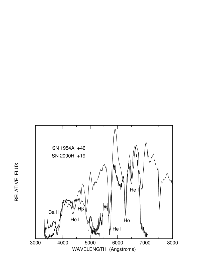
Figure 16: Transmission tracings of two $+46$ day photographic spectra of SN 1954A (dotted lines) are compared with the $+19$ day spectrum of SN 2000H (solid line).

SN 1954A appears to have been spectroscopically akin to SNe 2000H and 1999di. McLaughlin (1963) and Branch (1972) identified He I lines in photographic spectra of SN 1954A obtained at the Lick Observatory and the Mount Wilson and Palomar Observatories, respectively. Consequently SN 1954A usually has been regarded to have been a Type Ib supernova, but on occasion doubts has been expressed about the classification because of the low quality of the photographic spectra compared to modern observations. Figure 16 compares microphotometer tracings of the two earliest spectra of SN 1954A (Blaylock et al. 2000), obtained on blue– and red–sensitive emulsions 46 days after maximum light, with the $+19$ day spectrum of SN 2000H. Only this one spectrum of SN 1954 was obtained on a red–sensitive emulsion. The SN 1954A spectra are not actually relative flux but merely a measure of the transmission through the photographic plate. Parts of the spectra were overexposed so the features are distorted; in particular, emission peaks tend to be suppressed. The shapes of these spectra also are strongly influenced by the wavelength dependences of the emulsion sensitivities; e.g., neither emulsion is sensitive around 5200 Å and the sensitivity falls off steeply between 6500 and 7000 Å. Nevertheless, some of the absorptions in SN 1954A can be located and they correspond well with the absorptions in SN 2000H, including the two attributed to H$\alpha$ and H$\beta$. Branch (1972) considered the possibility of H$\alpha$ and H$\beta$ absorptions in SN 1954A, blueshifted by 10,800 km s^-1 in the observer’s frame; the value of $cz$ for the parent galaxy is now known to be 291 km s^-1, so the hydrogen lines are blueshifted by about 11,000 km s^-1 in the supernova frame. Branch also considered the possibility of Ne I lines in SN 1954A. This is perhaps still not ruled out, but given the apparent resemblance of SN 1954A to SNe 2000H, we prefer the hydrogen identification.

In terms of apparent magnitude, SN 1954A was the fourth brightest supernova of the twentieth century, surpassed only by the Type II SN 1987A and the Type Ia SNe 1972E and 1937C (Barbon et al. 1999). SN 1954A occurred in the star–bursting dwarf galaxy NGC 4214, at a distance of only about 4 Mpc (Leitherer et al. 1996), more than 10 times closer than SNe 2000H and 1999di, so it is more amenable to studies of the environment in which it exploded. We note that Van Dyk, Hamuy, & Filippenko (1996) found SN 1954A to be unusual among SNe Ib in that it was not near any visible H II region, and that a deep VLA search for radio emission at the site of SN 1954A carried out by J. Cowan and D. Branch in May, 1986, resulted in a three–sigma upper limit to the flux density at 20 cm of 0.068 mJy (Eck 1998), which corresponds to a monochromatic luminosity of less than one twentieth of Cas A.

5.3 Other Selected Comparisons

Figure 17 compares a spectrum of SN 1984L obtained 9 days after maximum with a synthetic spectrum that has $v_{phot}$=8000 km s^-1 and $T_{bb}$= 6500 K, and includes hydrogen lines detached at 15,000 km s^-1. The Fe II lines fit very well, and the fit to the other features is satisfactory. Given the presence of H$\alpha$ in SNe 2000H, 1999di, and 1954A, we assume that the 6300 Å absorption is produced by H$\alpha$. However, because the H$\alpha$ optical depth at the detachment velocity is only 0.6, there is no support for this identification from H$\beta$ because it is too weak to see. (The oscillator strength of H$\beta$ is about one fifth that of H$\alpha$.) Figure 18 compares the $+9$ day spectrum of SN 1984L with the $+5$ day spectrum of SN 2000H. The spectra are similar except that in SN 1984L the 6300 Å absorption is weaker and the 4560 Å absorption is not visible. This shows that while our assumption that the 6300 Å absorption in SN 1984L is produced by H$\alpha$ is reasonable, it is not proven. It is conceivable that C II $\lambda$6580 or (more plausibly because it wouldn’t need to be detached) Ne I $\lambda$6402 could be responsible for the 6300 Å absorption in SN 1984L and other typical SNe Ib, and be overwhelmed by H$\alpha$ only in events such as SNe 2000H, 1999di, and 1954A. We proceed on the assumption that at early times the 6300 Å absorption is produced by H$\alpha$ in all the SNe Ib of our sample.

As an example of a comparison at a earlier time when $v_{phot}$ is higher, Figure 19 compares the earliest spectrum for which good wavelength coverage is available, the Beijing spectrum of SN 1999dn 10 days before maximum, with a synthetic spectrum that has $v_{phot}$=14,000 km s^-1 and $T_{bb}$= 6500 K. Now hydrogen lines are detached at 18,000 km s^-1, where the H$\alpha$ optical depth is 1.3. The fit is good, except near 6600 Å.

Figure 20 compares a spectrum of SN 1998dt obtained 32 days after maximum with a synthetic spectrum that has $v_{phot}$= 9000 km s^-1 and $T_{bb}$= 5000 K. This comparison is shown because, as will be seen below, although the spectrum has a typical SN Ib appearance the inferred value of $v_{phot}$ is unusually high for a SN Ib this long after maximum. The fit to the Fe II features is unusually poor, but this value of $v_{phot}$ does give the best fit in the 4300 to 5300 Å region, and a significantly lower value would give a noticeably worse fit. (The narrow H$\alpha$ emission from an H II region in the parent galaxy is very close to 6563 Å, which shows that the high required value of $v_{phot}$ is not due to the observed spectrum having been inadvertently overcorrected for parent galaxy redshift.)

Now we briefly consider the events of our sample for which the times of maximum light are unknown. The spectrum of SN 1996N indicates that it was discovered not long after maximum. Because we use hydrogen lines in the synthetic spectrum for SN 1996N, the comparison with the observed spectrum is shown in Figure 21. Helium lines are undetached and the optical depth of the reference line is 5; hydrogen lines are detached at 17,000 km s^-1 where the optical depth of H$\alpha$ is 0.5. Overall, the fit is good.

SNe 1991ar and 1997dc do not appear to be unusual provided that they were discovered well after maximum light. As discussed by Matheson et al. (2001), the spectra of SN 1998T are seriously contaminated by light from the parent galaxy; taking this into consideration, SN 1998T does not appear to be unusual provided that it was discovered about a week after maximum. As far as we can tell, SNe 1991ar, 1997dc, and 1998T were typical SNe Ib, but they were not observed early enough to check on the presence of H$\alpha$.

6 RESULTS AND DISCUSSION

The most important of the fitting parameters that have been used for the synthetic spectra are collected in Table 2. The spectra are listed in order of time with respect to maximum light so only the supernovae for which we have an estimate of the time of maximum light appear in the table. (The date 0703, for example, refers to July 3.)

For the six SNe Ib for which we have estimates of the time of maximum light, $v_{phot}$ is plotted against time in Figure 22. The tightness of the relationship is striking. SN 1998dt at 32 days after maximum seems to stand out; otherwise, the scatter about the mean curve is about what should be expected from our nominal errors of 1000 km s^-1 in $v_{phot}$ and a few days in the dates of maximum light. For the simple case of constant opacity and a $v^{-n}$ density distribution, the velocity at the photosphere would decrease with time as $v_{phot}\propto t^{-2/(n-1)}$. The line in Figure 22, the best power–law fit to the data (excluding SN 1998dt at 32 days), corresponds to $n=3.6$. Considering that the opacity is not really constant, that the actual density distribution does not really follow a single power law over a wide velocity range, and that the best power–law index for fitting the spectra is not well constrained, not much significance should be attched to the difference between $n=3.6$ and $n=8$.

Our adopted values of $v_{phot}$ can be used to make rough estimates of the mass and kinetic energy above the photosphere. For spherical symmetry and a $v^{-n}$ density distribution, the mass (in $M_{\odot}$) and the kinetic energy (in 10⁵¹ ergs) above the electron–scattering optical depth $\tau_{es}$ are (Millard et al. 1999)

$$M=1.2\times 10^{-4}\ v_{4}^{2}\ t_{d}^{2}\ \mu_{e}\ {{n-1}\over{n-3}}\ \tau_{es},$$

$$E=1.2\times 10^{-4}\ v_{4}^{4}\ t_{d}^{2}\ \mu_{e}\ {{n-1}\over{n-5}}\ \tau_{es},$$

where $v_{4}$ is $v_{phot}$ in units of 10,000 km s^-1, $t_{d}$ is the time since explosion in days, $\mu_{e}$ is the mean molecular weight per free electron, and the integration is carried out to arbitrarily high velocity. If we assume that maximum light occurs 20 days after explosion, that $n=8$, that $\mu_{e}=8$ (e.g., half–ionized helium or singly ionized oxygen), and that $v_{phot}$ is at $\tau_{es}=1$, then at maximum light $v_{phot}$=10,000 km s^-1 (Figure 22) gives $M=0.5~{}M_{\odot}$ and $E=0.9\times 10^{51}$ ergs. At 20 days after maximum, using $v_{phot}$=7000 km s^-1 and keeping the other parameters the same gives $M=1.1~{}M_{\odot}$ and $E=0.9\times 10^{51}$ ergs. In reality, of course, the kinetic energy above the 7000 km s^-1 photosphere must be greater than that above the 10,000 km s^-1 photosphere. If we use $n=4$ instead of $n=8$ between 7000 and 10,000 km s^-1  then we obtain a total of $M=1.5~{}M_{\odot}$ and $E=1.4\times 10^{51}$ ergs above the 7000 km s^-1 photosphere.

Figure 22 provides some constraints on models of SNe Ib. The hydrodynamics must account for the velocity at the photosphere as a function of time, and the ensemble of SN Ib progenitors must be consistent with the tightness of the relationship. The small scatter suggests that the masses and the kinetic energies of the SNe Ib of our sample are similar, and it does not leave much room for the influence on $v_{phot}$ of departures from spherical symmetry.

Figure 23 shows the minimum velocities of the He I lines (squares when undetached and diamonds when detached). There appears to be a standard pattern (again with the possible exception of SN 1998dt at 32 days). Before and near the time of maximum the He I lines tend to be undetached. After maximum the lines tend to be detached, but the detachment velocities tend to decrease with time, from about 10,000 to 7000 km s^-1. This means that the fraction of helium in this velocity range that is in the lower levels of the optical He I lines is increasing with time faster than $t^{2}$. (The matter density is decreasing as $t^{-3}$ by expansion but the Sobolev optical depth also is proportional to $t$ because it is inversely proportional to the velocity gradient.) The increasing fraction of helium in the excited levels may be understandable in terms of the decreasing column depth between the nickel core and the helium layers, and the decreasing detachment velocity may mean that the fractional helium abundance is lower at lower velocities. In any case, some helium is present at least down to 7000 km s^-1. Our estimate above for the total mass above the 7000 km s^-1 photosphere was 1.1 to 1.5 M_⊙, which is a rough upper limit on the mass of helium above 7000 km s^-1. There could be more helium below 7000 km s^-1.

Figure 23 provides more constraints on models of SNe Ib. The radial profile of the helium abundance, together with that of the ⁵⁶Ni that is responsible for exciting it, should account for the He I velocities and optical depths (Table 2).

Figure 23 also shows the minimum velocities of the hydrogen lines (circles), which always are detached. In the three events for which we are convinced of the hydrogen identifications — SNe 2000H, 1999dn, and 1954A — the minimum hydrogen velocity is between 11,000 and 13,000 km s^-1. In the events in which we assume H$\alpha$ to be present at early times — SNe 1983N, 1984L, 1999dn, and 1996N (the latter is not shown in Figure 23 because the date of maximum light is unknown) — the detachment velocities tend to decrease with time but they are consistent with similar minimum velocities of the hydrogen. Thus the available evidence is consistent with the proposition that SNe Ib in general have hydrogen down to $11,000-13,000$ km s^-1. [For comparison, in the Type IIb SN 1993J the characteristic velocity of the ejected hydrogen was about 9000 km s^-1 (Patat et al. 1995; Utrobin 1996; Houck & Fransson 1996), and in the Type IIb SN 1996cb it was about 10,000 km s^-1 (Deng et al. 2001).] A challenge for those who study the complicated evolution of massive stars in binary systems (e.g., Podsiadlowski, Joss, & Hsu 1992; Nomoto, Iwamoto, & Suzuki 1995; Wellstein, Langer, & Braun 2001) is to understand why many or perhaps even all stellar explosions that develop strong He I lines should eject at least a small amount of hydrogen.

The hydrogen mass that is required to give an H$\alpha$ optical depth of unity depends on the fraction of hydrogen that is in the Balmer level. In LTE, with an electron density of $10^{9}$ cm^-3, the Balmer fraction peaks around $10^{-9}$ near 6000 K. In this case we estimate that a hydrogen mass on the order of $10^{-2}~{}M_{\odot}$ would be required. Non–LTE calculations that take nonthermal excitation into account are needed for a more reliable estimate of the hydrogen mass.

The optical depths of the helium lines, and especially the hydrogen lines, are not very high, even though the corresponding absorption features are distinct and fairly deep. This reflects a simple geometric aspect of supernova line formation: as explained in Jeffery & Branch (1990), absorption features formed by detached lines are deeper than those formed by undetached lines. This point is illustrated in Figure 24, which shows that when hydrogen is detached from the photosphere by a factor of two and H$\alpha$ has $\tau=2$, its absorption feature is deeper than that of an undetached H$\alpha$ that has $\tau=10$. The H$\alpha$ optical depths in our synthetic spectra for SNe 2000H, 1999di, and 1954A are not high, so if they were only mildly lower these events would look like typical SNe Ib. Similarly, moderately lower He I line optical depths would transform a SN Ib into a SN Ic.

Figure 24 also illustrates how undetached hydrogen lines are more “obvious” than detached lines. First, undetached lines have conspicuous narrow, rounded emission peaks while detached lines have inconspicuous broad, flat peaks. Note also that although the H$\alpha$ absorption is deeper in the detached spectrum, the H$\beta$ absorption is deeper in the undetached spectrum. This is because in the undetached spectrum the optical depth at the photosphere of H$\beta$ is about 2 while in the detached spectrum the optical depth at the detachment velocity is only about 0.4. An optical depth as low as 0.4 can produce only a shallow absorption, even when the line is detached. For these reasons, supernovae that have undetached hydrogen lines have obvious hydrogen lines and are classified as Type II. Supernovae that have detached hydrogen lines are classified as Type Ib because the presence of hydrogen is not immediately obvious, even when the H$\alpha$ absorption is as deep as it is in SNe 2000H, 1999di, and 1954A. SNe IIb are those that have undetached hydrogen lines when they are first observed. In some cases, whether an event is classified as Ib or IIb may depend on how early the first spectrum is obtained.

The implication of the previous paragraphs is that the spectroscopic differences between SNe IIb, the SNe Ib that have deep H$\alpha$ absorptions, and typical SNe Ib may be caused mainly by mild differences in the hydrogen mass. For a given kinetic energy, the lower the hydrogen mass the higher the minimum velocity of the ejected hydrogen. Similarly, the spectroscopic differences between typical SNe Ic and SNe Ib could be caused mainly by moderate differences in the helium mass. For example, Matheson et al. (2001) found higher blueshifts of the O I $\lambda$7773 line in SNe Ic than in SNe Ib. For a given kinetic energy, the lower the helium mass the higher the minimum velocity of the ejected helium, and therefore the higher the velocity of the ejected oxygen. These suggestions are not original to this paper, but they are strengthened by our finding that the H I and He I optical depths in SNe Ib are not very high. These suggestions also are not inconsistent with arguments, based on light curves, for the existence of different physical classes of hydrogen–poor events that cut across the conventional spectroscopic types (e.g., Clocchiatti & Wheeler 1997).

The number of SNe Ib for which good spectral coverage is available is still relatively small. More events should be observed to explore the degree of the spectral homogeneity and to find out whether there is a continuum of hydrogen line strengths. Also needed are detailed non–LTE spectrum calculations for supernova models having radially stratified compositions, — to determine the the hydrogen and helium masses and the distribution of the ⁵⁶Ni that is required to excite the helium. The possibility that nonthermally excited Ne I can produce spectral features strong enough to be seen needs to be investigated. Detailed non–LTE calculations for parameterized SN Ib models, using the PHOENIX code (e.g., Baron et al. 1999), are underway.

This material is based upon work supported by the National Science Foundation under Grants No. AST–9986965 and AST–9731450 at Oklahoma and AST–9987438 at Berkeley. A.V.F. is grateful to the Guggenheim Foundation for a Fellowship.

Table 1: Type Ib Supernovae

SN	Galaxy	$cz$ (km s-1)	tmax
1954A	NGC 4214	291	April 21
1983N	NGC 5236	513	July 17
1984L	NGC 991	1534	August 22
1991ar	IC 49	*4520	*September 2
1996N	NGC 1398	1491	*March 12
1997dc	NGC 7678	3480	*August 5
1998T	NGC 3690	*3080	*March 3
1998dt	NGC 945	*4580	September 12
1999di	NGC 776	*4920	July 27
1999dn	NGC 7714	2700	August 31
2000H	IC 454	3894	February 11

Table 2: Synthetic Spectrum Parameters

SN	date	epoch	$v_{phot}$	$\tau$(He I)	$v_{det}$(He I)	$\tau$(H)	$v_{det}$(H)
1983N	0703	-14	17000
1983N	0706	-11	13000
1999dn	0821	-10	14000	2.0	14000	1.5	18000
1983N	0713	-4	11000
1983N	0717	0	11000	2.5	11000	0.8	15000
2000H	0211	0	11000	1	11000	6.0	13000
1999dn	0831	0	10000	5.0	11000	1.0	14000
1983N	0719	2	10000	4.0	10000	0.7	14000
2000H	0216	5	8000	2.0	9000	2.5	13000
1984L	0830	8	9000	2.0	10000	0.6	15000
1998dt	0920	8	9000	4.0	11000
1984L	0831	9	8000	1.5	10000	0.6	15000
1983N	0727	10	7000	7.0	8000	0.6	12000
1999dn	0910	10	7000	3.0	8000
1984L	0903	12	7000	1.0	9000	0.5	14000
1999dn	0914	14	6000	10	7000
1999dn	0917	17	6000	10	8000
2000H	0302	19	6000	5.0	8000	2.0	13000
1999di	0817	21	7000	10	8500	4.0	12000
1984L	0919	28	5000
2000H	0313	30	5000	3.0	7000	1.5	13000
1984L	0923	32	5000	5.0	7000
1998dt	1015	33	9000	10	9000
1984L	0928	37	5000	10	6000
1999dn	1008	38	6000	10	7000
1999di	0910	45	6000	10	7000	2.0	12000
2000H	0330	47	5000	1.0	7000	0.5	12000
1999di	0917	52	6000	10	7000	1.0	12000
2000H	0408	56	4000
1984L	1018	57	4000

Figure 1: A spectrum of SN 1996N obtained at the Anglo–Australian Observatory by Germany et al. (1999) on 1996 March 23, 11 days after discovery. The flux is in units of $10^{-17}$ erg cm^-2 s^-1 Å^-1. All spectra displayed in this paper have been deredshifted.

Figure 2: Spectra evolution of SN 2000H. The times are in days after 2000 February 11. The flux is in units of $10^{-16}$ erg cm^-2 s^-1 Å^-1. The ordinate refers to the first spectrum ($+0$ days) and the other spectra have been shifted downward by 0.6, 1.1, 1.4, 2.6, and 2.9 dex. The spectra were obtained as follows: $0$ days, Asiago 1.82m+AFOSC, res. 20 Å; $+5$ days, Danish1.54m+DFOSC, res. 11 Å; $+19$ days, ESO3.6m+EFOSC2, res. 15 Å; $+30$ days (average of two spectra taken on two consecutive nights), Danish1.54m+DFOSC, res. 11 Å; $+47$ and $+56$ days, ESO3.6m+EFOSC2, resol. 15 Å. The telluric absorptions have been removed.

Figure 3: The $+17$ day spectrum of SN 1999dn (solid line) is compared with a synthetic spectrum (dotted line) that has $v_{phot}=6000$ km s^-1 and $T_{bb}=4800$ K, and contains lines of He I, O I, Ca II, Sc II, Ti II, and Fe II.

Figure 4: Like Figure 3, but with only the Fe II lines in the synthetic spectrum.

Figure 5: A comparison of Fe II synthetic spectra having $v_{phot}=5000$ (dotted line) and 10,000 km s^-1 (solid line).

Figure 6: Like Figure 3, but with only the He I lines in the synthetic spectra, detached at 8000 km s^-1 (top panel) and undetached (bottom panel).

Figure 7: Like Figure 3, but with only the O I lines (top panel) and the Ca II lines (bottom panel) in the synthetic spectra.

Figure 8: Like Figure 3, but with only the Ti II lines (top panel) and the Sc II lines (bottom panel) in the synthetic spectra.

Figure 9: Like Figure 3, but with $n=5$ instead of $n=8$.

Figure 10: The $+5$ day spectrum of SN 2000H (solid line) is compared with a synthetic spectrum (dotted line) that has $v_{phot}=8000$ km s^-1 and $T_{bb}=6500$ K, and contains lines of H, He I, O I, Ca II, Sc II, Ti II, and Fe II.

Figure 11: Like Figure 10, but a better view of the H$\beta$ region.

Figure 12: The $+21$ day spectrum of SN 1999di (solid line) is compared with the $+19$ day spectrum of SN 2000H (dotted line).

Figure 13: The $+21$ day spectrum of SN 1999di (solid line) is compared with a synthetic spectrum (dotted line) that has $v_{phot}=7000$ km s^-1 and $T_{bb}=4500$ K, and contains lines of H, He I, O I, Ca II, Sc II, Ti II, and Fe II.

Figure 14: Like Figure 12, but a better view of the H$\beta$ region.

Figure 15: The $+21$ day spectrum of SN 1999di (solid lines) is compared with synthetic spectra (dotted lines) that contain only lines of C II (top panel) and Ne I (bottom panel).

Figure 17: The $+9$ day spectrum of SN 1984L (solid line) is compared with a synthetic spectrum (dotted line) that has $v_{phot}=9000$ km s^-1 and $T_{bb}=8500$ K, and contains lines of H, He I, O I, Ca II, Sc II, Ti II, and Fe II.

Figure 18: The $+9$ day spectrum of SN 1984L (dotted line) is compared with the $+5$ day spectrum of SN 2000H (solid line).

Figure 19: The $-10$ day spectrum of SN 1999dn (solid line) is compared with a synthetic spectrum (dotted line) that has $v_{phot}=14,000$ km s^-1 and $T_{bb}=6500$ K, and contains lines of H, He I, O I, Ca II, and Fe II.

Figure 20: The $+32$ day spectrum of SN 1998dt (solid line) is compared with a synthetic spectrum (dotted line) that has $v_{phot}=9000$ km s^-1 and $T_{bb}=5000$ K, and contains lines of He I, O I, Ca II, Sc II, Ti II, and Fe II.

Figure 21: The 1996 March 23 spectrum of SN 1996N (solid line) is compared with a synthetic spectrum (dotted line) that has $v_{phot}=9000$ km s^-1 and $T_{bb}=5000$ K, and contains lines of H, He I, O I, Ca II, and Fe II.

Figure 22: The velocity at the photosphere, as inferred from Fe II lines, is plotted against time after maximum light. The line is a power–law fit to the data, with SN 1998dt at 32 days (open circle) excluded.

Figure 23: The minimum velocity of the He I lines (filled squares when undetached, filled triangles when detached) and the minimum velocity of the hydrogen lines (open circles; always detached) are plotted against time after maximum light. The curve is the power–law fit to the velocity at the photosphere, from Figure 22.

Figure 24: A synthetic spectrum (dotted line) that has $v_{phot}$=10,000 km s^-1 and hydrogen lines detached at 20,000 km s^-1, where $\tau$(H$\alpha$)=2, is compared with a synthetic spectrum (solid line) that has $v_{phot}$=10,000 km s^-1 and undetached hydrogen lines, with $\tau$(H$\alpha$)=10 at the photosphere.

References

- (1)
- (2) Barbon, R., Buondi, V., Cappellaro, E., & Turatto, M. 1999, A&AS, 139, 531
- (3)
- (4) Baron, E., Branch, D., Hauschildt, P. H., Filippenko, A. V., & Kirshner, R. P. 1999, ApJ, 527, 739
- (5)
- (6) Benetti, S., Cappellaro, E., Turatto, M., & Pastorello, A. 2000, IAU Circ. 7375
- (7)
- (8) Blaylock, M., Branch, D., Casebeer, D., Millard, J., Baron, E., Richardson, D., & Ancheta, C. 2000, PASP, 112, 1439
- (9)
- (10) Branch, D. 1972, A&A, 16, 247
- (11)
- (12) Branch, D. 2001, in Supernovae and Gamma–Ray Bursts: The Largest Explosions in the Universe, ed. M. Livio (Cambridge: Cambridge University Press), in press
- (13)
- (14) Casebeer, D., Branch, D., Blaylock, M., Millard, J., Baron, E., Richardson, D., & Ancheta, C. 2000, PASP, 112, 1433
- (15)
- (16) Clocchiatti, A. & Wheeler, J. C. 1997, in Thermonuclear Supernovae, ed. P. Ruiz–Lapuente, R. Canal, & J. Isern (Dordrecht: Kluwer), p. 863
- (17)
- (18) Deng, J. S., Qiu, Y. L., Hu, J. Y., Hatano K., & Branch D. 2000, ApJ, 540, 452
- (19)
- (20) Deng, J., Qiu, Y., & Hu, J. 2001, preprint
- (21)
- (22) Eck, C. R. 1998, PhD Thesis, University of Oklahoma
- (23)
- (24) Filippenko, A. V. 1997, ARAA, 35, 309
- (25)
- (26) Filippenko, A. V., et al., 1992, AJ, 104, 1543
- (27)
- (28) Fisher, A. 2000, PhD Thesis, University of Oklahoma
- (29)
- (30) Garnavich, P. M., et al., 2001, ApJ, submitted
- (31)
- (32) Garnavich, P., Challis, P., Jha, S., & Kirshner, R. 2000, IAU Circ. 7366
- (33)
- (34) Germany, L., Schmidt, B., Stathakis, R., & Johnston, H. 2000, IAU Circ. 6351
- (35)
- (36) Harkness, R. P., et al., 1987, ApJ, 317, 355
- (37)
- (38) Hatano, K., Branch, D., Fisher, A., Millard, J., & Baron, E. 1999, ApJS, 121, 233
- (39)
- (40) Houck, J. C., & Fransson, C. 1996, ApJ, 456, 811
- (41)
- (42) Jeffery, D. J., & Branch, D. 1990, in Supernovae, ed. J. C. Wheeler, T. Piran, & S. Weinberg (Singapore: World Scientific), p. 149
- (43)
- (44) Kurucz, R. L. 1993, CDROM No. 1: Atomic Data for Opacity Calculations, Cambridge, Smithsonian Astrophysical Observatory
- (45)
- (46) Leitherer, C., Vacca, W. D., Conti, P. S., Filippenko, A. V., Robert, C., & Sargent, W. L. W. 1996, ApJ, 465, 717
- (47)
- (48) Lucy, L. B. 1991, ApJ, 383, 308
- (49)
- (50) Matheson, T., Filippenko, A. V., Li, W., Leonard, D. C., & Shields, J. C. 2001, AJ, 121, 1648
- (51)
- (52) McLaughlin, D. B. 1963, PASP, 75, 133
- (53)
- (54) Millard, J., et al., 1999, ApJ, 527, 746
- (55)
- (56) Nomoto, K., Iwamoto, K., & Suzuki, T. 1995, Phys. Rep., 256. 173
- (57)
- (58) Pastorello, A., Altavilla, G., Cappellaro, E., & Turatto, M. 2000, IAU Circ. 7367
- (59)
- (60) Patat, F., Chugai, N., & Mazzali, P. A. 1995, A&A, 299, 715
- (61)
- (62) Podsiadlowski, Ph., Joss, P. C., & Hsu, J. J. L. 1992, ApJ, 391, 246
- (63)
- (64) Qiu, Y., Li, W., Qiao, Q., & Hu, J. 1999, AJ, 117, 736
- (65)
- (66) Richter, T., & Sadler, E. M. 1983, A&A, 128, L3
- (67)
- (68) Swartz, D. A., Filippenko, A. V., Nomoto, K., & Wheeler, J. C. 1993, ApJ, 411, 313
- (69)
- (70) Tsvetkov, D. Yu. 1987, Sov. Astron. Lett., 13, 376
- (71)
- (72) Utrobin, V. P. 1996, A&A, 306, 219
- (73)
- (74) Van Dyk, S., Hamuy, M., & Filippenko, A. V. 1996, AJ, 111, 2017
- (75)
- (76) Wellstein, S., Langer, N., & Braun, H. 2001, A&A, 369, 939
- (77)
- (78) Wheeler, J. C., Harkness, R. P., Clocchiati, A., Benetti, S., Brotherton, M. S., DePoy, D. L., & Elias, J. 1994, ApJ, 436, L135
- (79)
- (80) Woosley, S. E., & Eastman, R. G. 1997, in Thermonuclear Supernovae, ed. P. Ruiz–Lapuente, R. Canal, & J. Isern (Dordrecht: Kluwer), p. 821
- (81)