Gravitational wave background from coalescing compact stars in eccentric orbits

Abstract

Stochastic gravitational wave background produced by a stationary coalescing population of binary neutron stars in the Galaxy is calculated. This background is found to constitute a confusion limit within the LISA frequency band up to a limiting frequency $\nu_{lim}{}\sim 10^{-3}$ Hz, leaving the frequency window $\sim 10^{-3}$–$10^{-2}$ Hz open for the potential detection of cosmological stochastic gravitational waves and of signals involving massive black holes out to cosmological distances.

1 Introduction

In a short time, gravitational wave astronomy is expected to start collecting first data from different astrophysical sources of gravitational radiation, most probably from coalescing binary neutron stars and black holes (for a recent review, see Grishchuk et al. 2001). The first large gravitational wave (GW) interferometers LIGO, VIRGO, GEO-600 and TAMA-300 will be sensitive to dimensionless metric variations in the frequency range 10-1000 Hz at a level of $h\sim 10^{-21}$ (Braginsky 2000 and references therein). Due to seismic noise limitations lower frequencies ($10^{-4}-10^{-1}$ Hz) can be studied only with space-born antennas, such as LISA laser interferometer (Bender et al. 2000). Prospects for finding astrophysical sources within the LISA frequency band are very good, especially for supermassive binary black holes which can be observed by LISA with a record signal-to noise ratio of order 1000 from cosmological distances (Vecchio et al. 1997).

In addition to signals from individual sources, GW interferometers can detect stochastic gravitational waves. Such waves (GW backgrounds, or GW noises) can be produced by a large collection of unresolved individual sources, e.g. by binary stars (Mironovskij 1965, Lipunov and Postnov 1987, Bender and Hils 1997, Kosenko and Postnov 1998) or rapidly rotating neutron stars (Giazotto et al. 1997, Postnov and Prokhorov 1997, Ferrari et al. 1999). These GW backgrounds are usually considered as unwanted additional noises to the intrinsic noises of GW detectors, since they could potentially mimic stochastic GW backgrounds of cosmological origin (primordial or relic GW) that bring a valuable information about physical processes in the very early Universe (Grishchuk et al. 2001 and references therein).

Ordinary galactic binaries, in which at least one of the component is a normal main-sequence star, mostly contribute at low-frequency band ($\nu\sim 10^{-7}-10^{-5}$ Hz) (Mironovskij 1965). At higher frequencies $10^{-4}-10^{-2}$ Hz compact coalescing white dwarf (WD) binaries should form a noticeable background above the LISA noise curve (Lipunov and Postnov 1987, Bender and Hils 1997, Grishchuk et al. 2001). Generally, the level of the GW noise within a fixed frequency interval from a collection of $N$ unresolved independent sources in terms of dimensionless amplitude is $h\propto\sqrt{N}$. In case of binaries that loose the orbital angular momentum due to gravitational radiation back reaction, this level is $h\propto\sqrt{\cal R}$, where $\cal R$ is the coalescing rate of these binaries (see Grishchuk et al. 2001 for more detail).

Another important quantity is the upper frequency $\nu_{lim}{}$ above which each individual source can be resolved during one-year observation time (i.e. within the frequency bin $\Delta\nu=3\times 10^{-8}$ Hz). In fact, it is this limiting frequency which mostly relate to the challenging task of detection of a relic GW background: at $\nu>\nu_{lim}{}$ we will be able in principle to single out individual sources and thus have prospects to register cosmological GW noise using one interferometer (Grishchuk et al. 2001).

The obvious condition for $\nu_{lim}{}$ reads ${\cal R}\Delta T(\nu_{lim}{})=1$, where $\Delta T(\nu)$ is the time each source ‘spends‘ within the frequency bin at a given frequency $\nu$. For example, in the simplest case of a collection of galactic binary WD in circular orbits which coalesce at a constant rate ${\cal R}={\cal R}_{300}\times(1/300)$ yr^-1

$$\begin{array}[]{rl}\nu_{lim}{}(\hbox{WD})&\approx(1.2\times 10^{-3}\hbox{Hz})~{}{\cal R}_{300}^{3/11}\\ &\times\left(\frac{\Delta\nu}{3\times 10^{-8}\hbox{Hz}}\right)^{3/11}\left(\frac{\cal M}{0.52M_{\odot}}\right)^{-5/11}\end{array}$$

where $\cal M$ is the chirp mass of the binary. For merging binary neutron stars (NS) $\nu_{lim}{}$ calculated as above would give even smaller value, $\nu_{lim}{}($NS$)=3\times 10^{-4}$ Hz, since the binary NS coalescence rate in most optimistic scenarios is ${\cal R}_{NS}{}\sim 10^{-4}$ yr^-1 (Grishchuk et al. 2001, Kalogera et al. 2000). Note that the uncertainty in this rate by a factor of 3 or so is of minor importance since $\nu_{lim}{}\propto{\cal R}^{3/11}$.

However, there is an important difference between the merging WD and NS. Binary WD must have almost circular orbits from the very beginning since they result from a spiral-in process during the common envelope stage. Unlike binary WD, binary NS must have (and this is what we actually observe in the known binary radiopulsars with NS companions) a significant eccentricity at birth, since they are formed after two supernova explosions with substantial mass loss from the system. The possible asymmetry of supernova explosion leading to the natal kick velocity of newborn NS additionally affects the orbital parameters leading to higher orbital eccentricities.

It is well known (Peters and Mathews 1963) that an eccentric binary system emit GW in a wide frequency band. This means that the high-order harmonics from an eccentric binary system should be observed at frequencies $\nu>2\nu_{K}$ ($2\nu_{K}$ is twice the Keplerian orbital frequency at which a circular binary radiates GW), so the entire population of galactic eccentric binary NS should contribute in a broader frequency band than analogical circular binaries would do. The effect may be not small, since the total number of NS+NS binaries in the Galaxy is quite large, as the simple estimate below shows. Assume the stationary formation rate ${\cal R}_{f}$ of NS binaries in the Galaxy (which is a reasonable approximation during at least the last 5 billion years). Then the total number of them is of order ${\cal R}_{f}\times T_{gal}$, where $T_{gal}$ is the galactic age. Note that the actual NS formation rate is higher than the NS merging rate ${\cal R}_{NS}{}$ since a NS binary could merge only if its initial semi-major axis $a_{i}$ and eccentricity $e_{i}$ satisfy the condition $T_{coal}(a_{i},e_{i})<t_{gal}$, where $T_{coal}$ is the time the systems takes from the formation to coalescence due to GW orbit decay. So the minimum number of NS binaries in the Galaxy is estimated to be of order ${\cal R}_{NS}{}\times T_{gal}=10^{-4}\times 10^{10}\sim 10^{6}$.

To calculate the GW background produced by binary NS, the following steps should be done. (1) NS binaries form with some initial distribution over orbital semi-major axes and eccentricities $F_{in}(a,e)$. This distribution can be found from evolutionary calculations using e.g. binary population synthesis method (Lipunov et al. 1996). (2) Next, if orbital parameters of such binaries evolve only due to GW emission, a stationary distribution function $F_{st}(a,e)$ can be recovered (Buitrago et al. 1994). (3) Knowing the GW spectrum of a binary with given $(a,e)$ (Peters and Mathews 1963), the final GW noise from these sources can be computed.

In the present paper we specially focus on the effect of eccentricity of coalescing NS binaries on the level and limiting frequency of the stochastic GW background they form. We find, as expeted, that the level of this background is lower than from coalescing galactic binary WD, and the limiting frequency $\nu_{lim}(e\neq 0)$ is higher than calculated for circular case. The initial (model-dependent) distribution of NS binaries only slightly affects the result. This leaves the frequency interval $\sim 10^{-3}-10^{-2}$ Hz open for searches of primordial GW backgrounds.

2 Initial galactic binary NS distribution

To calculate the initial binary NS distribution $F_{in}(a,e)$ in the Galaxy we used the population synthesis method described by many authors (Lipunov, Postnov, Prokhorov 1996; Lipunov, Postnov, Prokhorov 1997; Portegies Zwart, Yungelson 1998). It uses the simulation of evolution of a large number of binaries with initial parameters (masses of the components, semimajor axes, eccentricities etc.) distributed according to some (taken from observations or model) laws. There are also evolutionary parameters, such as efficiency of common envelope stage, kick velocity during supernova explosion, initial spin of compact objects, etc. (see Grishchuk 2001 for more detail), of which kick velocity imparted to compact object (neutron star or black hole) at birth mostly impacts the resulting distribution $F_{in}(a,e)$. We assumed a Maxwellian form of the kick velocity distribution and varied its amplitude $v_{k}$ from 0 to 400 km/s. The resulting normalized initial distribution $F_{in}(a,e)$ for $v_{k}=200$ km/s is shown in Fig. 1.

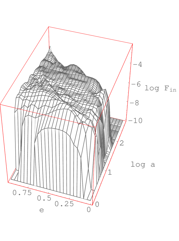
Figure 1: The initial binary NS distribution $F_{in}(a,e)$ for the kick velocity amplitude $v_{k}=200$ km/s. Initial semimajor axis $a$ is in solar units.

NS binaries are formed in a very broad interval of $a$ and $e$, but interesting for us here will be only those that can coalesce over the galactic age $T_{coal}<T_{gal}$, since only such binaries can form a stationary distribution. It is seen from Fig. 1 that most binaries form with small or moderate eccentricities ($e<0.5$) in a wide range of semimajor axes $a_{in}\sim 1-300R_{\odot}$. Increase in the kick velocity amplitude broadens the initial distribution function over eccentricity.

3 Stationary binary NS distribution

GW back reaction causes orbital decay of binary system. For an eccentric binary star, this can be described in quadrapole approximation by ordinary differential equations for orbital semimajor axis and eccentricity (Peters & Mathews, 1963):

$$\frac{da}{dt}=-\frac{64}{5}\frac{G^{3}m_{1}m_{2}(m_{1}+m_{2})}{c^{5}a^{3}(1-e^{2})^{7/2}}(1+\frac{73}{24}e^{2}+\frac{37}{96}e^{4})$$ (1)

$$\frac{de}{dt}=\frac{304}{15}\frac{G^{3}m_{1}m_{2}(m_{1}+m_{2})e}{c^{5}a^{4}(1-e^{2})^{5/2}}(1+\frac{121}{304}e^{2})$$ (2)

Given the initial function $F_{in}(a,e)$, it is straightforward to find a stationary distribution function $F_{st}(a,e)$ (Buitrago et al. 1994):

$$\begin{array}[]{r@{}l}F_{st}(a,e)=&\frac{\displaystyle 15c^{5}{\cal R}_{f}}{\displaystyle 304G^{3}m_{1}m_{2}(m_{1}+m_{2})}\\[5.69054pt] &\times\frac{\displaystyle a^{4}(1-e^{2})^{7/2}}{\displaystyle e^{31/19}(1+\frac{\displaystyle 121}{\displaystyle 304}e^{2})^{3169/2299}}\\[8.53581pt] &\times\int\limits_{0}^{1}\frac{\displaystyle z^{12/19}(1+\frac{\displaystyle 121}{\displaystyle 304}z^{2})^{870/2299}}{\displaystyle 1-z^{2}}F_{in}(a(z),z)\,dz\end{array}$$ (3)

At present, only some fraction of systems from the initial distribution with $T_{coal}<T_{gal}$ reaches stationarity. The function $F_{st}(\nu_{K},e)$ is calculated for this part of $F_{in}(a,e)$ from Fig. 1 and is shown in Fig. 2. In this figure we use the Keplerian frequency $\nu_{K}=\sqrt{(1/2\pi)G(m_{1}+m_{2})/a^{3}}$ instead of the semi-major axis $a$.

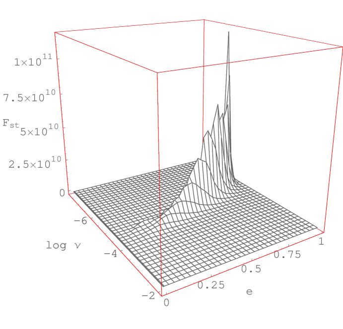
Figure 2: The stationary distribution function $F_{st}$ for binary NS in eccentric orbits which coalesce due to GW emission in a time interval shorter than the galactic age $10^{10}$ years.

4 GW spectrum from non-circular binary stars

In the simplest case of two point masses in a circular orbit, the energy losses caused by the quadrupole gravitational wave emission $L_{0}=\frac{\displaystyle dE}{\displaystyle dt}(\nu_{K})$ are defined by (Einstein, 1916, 1918; Landau & Lifshiz 1971):

$$L_{0}=\frac{32}{5}\frac{G^{4}}{c^{5}}\frac{m_{1}^{2}m_{2}^{2}(m_{1}+m_{2})}{a^{5}}$$ (4)

where $G$ is Newton’s gravitational constant, $c$ is the speed of the light in a vacuum and $m_{1},m_{2}$ are the masses of stars. All GW radiation in this case is emitted at a single frequency $2\nu_{K}$.

For a non-circular orbit with eccentricity $e$ the GW luminosity increases (Peters & Mathews 1963):

$$\frac{dE}{dt}=L_{0}\times\frac{1+\frac{\displaystyle 73}{\displaystyle 24}e^{2}+\frac{\displaystyle 37}{\displaystyle 96}e^{4}}{(1-e^{2})^{7/2}}$$ (5)

The emission now is widely spread over higher-order harmonics to the main frequency (Peters & Mathews 1963):

$$\frac{dE}{dt}(\nu=n\nu_{k})=L_{0}\times g(n,e)$$ (6)

$$g(n,e)=\frac{n^{4}}{32}([J_{n-2}(ne)-2eJ_{n-1}(ne)+\frac{2}{n}J_{n}(ne)$$

$$+2eJ_{n+1}(ne)-J_{n+2}(ne)]^{2}+(1-e^{2})[J_{n-2}(ne)$$

$$-2J_{n}(ne)+J_{n+2}(ne)]^{2}+\frac{4}{3n^{2}}{J_{n}}^{2}(ne))$$ (7)

Here $J_{n}$ is Bessel function and $n$ is the number of the harmonics.

The total energy emitted per second in a frequency interval $\Delta\nu$ by all binaries in the Galaxy is

$$\begin{array}[]{l}\frac{\displaystyle dE}{\displaystyle dt}=\int\limits_{\nu}^{\nu+\Delta\nu}\biggl{(}~{}\sum\limits_{n=1}^{\infty}\int\limits_{0}^{1}L_{0}(\frac{\displaystyle\nu}{\displaystyle n})\,g(n,e)\,F_{st}(\frac{\displaystyle\nu}{\displaystyle n},e)\,de\biggr{)}\,\frac{\displaystyle d\nu}{\displaystyle n}\\ \approx\biggl{(}~{}\sum\limits_{n=1}^{n_{lim}}\int\limits_{0}^{1}L_{0}(\frac{\displaystyle\nu}{\displaystyle n})\,g(n,e)\,F_{st}(\frac{\displaystyle\nu}{\displaystyle n},e)\,de\biggr{)}\frac{\displaystyle\Delta\nu}{\displaystyle n}\\ \end{array}$$ (8)

where $F_{st}(\frac{\displaystyle\nu}{\displaystyle n},e)\equiv F_{st}(\nu_{k},e)$ is a stationary distribution function of binary NS. In the last equation we take into account $\Delta\nu\ll\nu$. The amplitude of high-order harmonics rapidly decreases, so we stopped the summation of harmonics for $n>n_{lim}$, $n_{lim}:g(n_{lim},e)=\epsilon\times\max_{n}[g(n,e)]$. We assumed $\epsilon=10^{-4},10^{-6},10^{-10}$. Decreasing $\epsilon$ increases the total number of harmonics which contribute to the given frequency bin, but practically does not change the number of the most powerful harmonics within it (see Fig. 7).

5 Stationary stochastic GW noise from coalescing binary NS

First, consider the GW spectrum from a delta-function initial distribution: $F_{in}(a,e)=\delta(a-a_{0},e-e_{0})$, that is assume all binaries to form at one point $(a_{0},e_{0})$ in $(a-e)$ configuration space at a rate of ${\cal R}_{NS}{}=10^{-4}$ yr^-1. The spectrum formed by the first three harmonics and the total stationary GW background for this case are shown in Fig. 3 and Fig. 4 for $a_{0}=5R_{\odot}$ and $e_{0}=0.5,~{}0.9$, respectively. It is seen that increase in the initial eccentricity strongly affects the shape of the spectrum up to some frequency at which the eccentricities of binaries in the stationary distribution become sufficiently small. Above this frequency only the second harmonics from almost circular binaries contributes to the total spectrum. The non-monotonic dependence of the spectrum formed by the harmonics is due to the non-monotonic behaviour of the energy emitted at each harmonics with eccentricity (Eq. (6)-(4)).

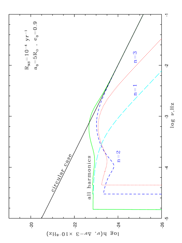
Figure 3: The resulting GW spectrum and the contribution from the first, second and third harmonics. All systems form with $a_{0}=5R_{\odot},e_{0}=0.9$. For comparison we show the spectrum for circual NS binaries coalescing with the same rate, and with initial orbital periods longer than $2\times 10^{5}$s.

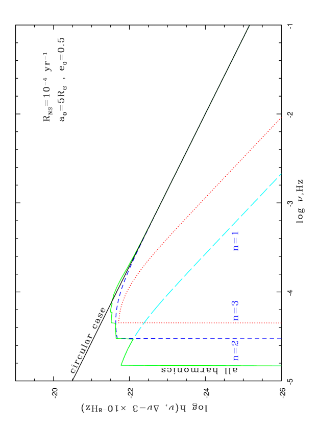
Figure 4: The same as in Fig 3 for systems with $a_{0}=5R_{\odot},e_{0}=0.5$.

Now we turn to the expected GW stochastic background from galactic NS binaries. We shall assume all the sources to lie at one distance $r=7.9$ kpc, which is close to the average distance to stars in our Galaxy. This simplifying assumption is unlikely to change our general conclusions. At each frequency $\nu$ we sum up the GW flux from all the harmonics that fall within the chosen frequency bin $\Delta\nu=3\times 10^{-8}$ Hz from lower-frequency non-circular systems in the calculated stationary distribution $F_{st}(\nu,e)$ (Eq. (3)), as modified by including only the part that has come to equilibrium in the lifetime of the galaxy, as discussed earlier.

The resulting noise curve is shown in Fig. 5 in terms of dimensionless amplitude $h$

$$h^{2}(\nu)=\frac{G}{c^{3}r^{2}(\pi\nu)^{2}}\frac{dE}{dt}$$ (9)

As expected, the NS+NS confusion noise lies below WD+WD curve, mainly due to lower ${\cal R}_{NS}{}$. High-order harmonics from non-circular NS binaries mostly contribute at lower frequencies, so starting from $\nu\sim 10^{-4}$ Hz the calculated noise curve practically coincides with that formed by circular NS binaries coalescing with the same rate ${\cal R}_{NS}{}=10^{-4}$ yr^-1.

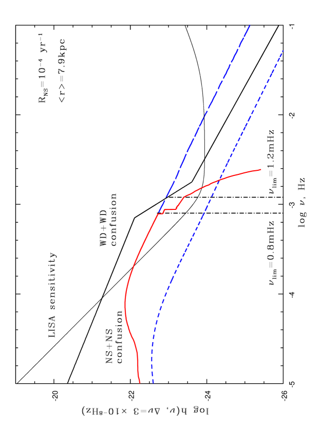
Figure 5: GW background from stationary binary NS population calculated for a model spiral galaxy with the NS+NS coalescing rate ${\cal R}_{NS}=10^{-4}$ yr^-1. The limiting frequecy above which the most powerful harmonics can be resolved in one-year observation is $\nu_{lim}{}\simeq 0.8$ mHz. If no harmonics were subtracted from the frequency bin $3\times 10^{-8}$ Hz, the background would continue toward higher frequencies as shown by the long-dashed line. THe lower dashed line shows contribution from extragalactic NS+NS binaries. The upper solid line schematically represents WD+WD confusion limit from Bender and Hils (1997) ($\nu_{lim}{}\simeq 1.2$ mHz, Eq. (1)). The proposed LISA sensitivity is from Thorne (1995) [Fig. 14]

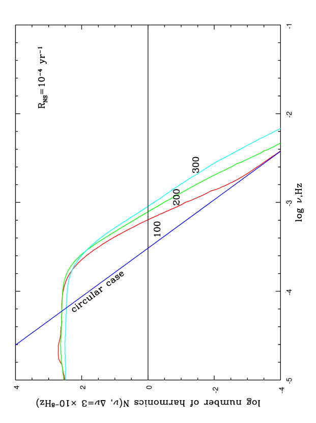
Figure 6: Number of harmonics from non-circular galactic NS binaries producing the stochastic noise in the frequency bin $\Delta\nu=3\times 10^{-8}$ Hz as a function of the kick velocity. The curves are labeled with kick velocity amplitudes $100,200$ and $300$ km/s assumed in the population synthesis calculations. The straight line is for the circular NS binaries. The limiting frequency $\nu_{lim}$ above which individual harmonics can be resolved follows from the condition $N(\nu_{lim},\Delta\nu)=1$.

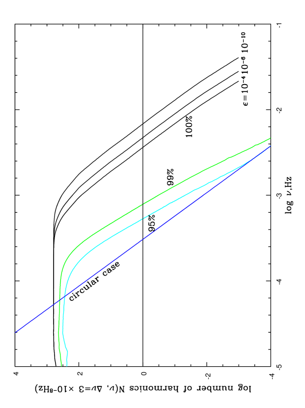
Figure 7: Number of the most powerful harmonics from non-circular galactic NS binaries which contribute 95%, 99% and 100% of the total GW energy collected in the bin $\Delta\nu=3\times 10^{-8}$ Hz. The effect of increase in the number of harmonics $n_{lim}$ determining the total energy collected in the bin (Eq. (9)) is shown for the total number of harmonics (100%) for different $\epsilon$. Kick velocity amplitude $200$ km/s.

More important in the non-circular case is the increase of the limiting frequency $\nu_{lim}{}$ above which individual sources can be resolved during a one-year observation. To estimate it, we calculate the number of harmonics inside the frequency bin $\Delta\nu$. Formally, this number is more than one at any frequency, but at high frequencies the main contribution must come from circular binaries (2-nd harmonics), the total GW power from higher-order harmonics from low-frequency eccentric systems becoming gradually less and less. So the number of harmonics contributing in a given frequency bin $\Delta\nu=3\times 10^{-8}$ Hz were counted, starting with the strongest one and continuing until 99bin (Eq.(8)) had been included. The number of such harmonics as a function of frequency and the assumed kick velocity amplitude $N(\nu,\Delta\nu)$ is shown in Fig. 6. The limiting frequency $\nu_{lim}{}$ is determined from equation $N(\nu_{lim}{},\Delta\nu)=1$. To within uncertainties of our calculations (${\cal R}_{NS}{},F_{in}(a,e)$, etc.), $\nu_{lim}{}\simeq 10^{-3}$ Hz, close to the break in the confusion limit from binary WD. For comparison, in the same Fig. 6 we show $N(\nu,\Delta\nu)$ for stationary circular NS binaries coalescing with the same rate ${\cal R}_{NS}{}=10^{-4}$ yr^-1 ($\nu_{lim}{}({e=0})\propto 3\times 10^{-4}$ Hz). The effect of increasing the chosen level for the GW power from the strongest harmonics in the bin is illustrated in Fig. 7. Increasing the level from 95% to 100% changes the limiting frequency $\nu_{lim}{}$ by almost an order of magnitude.

This procedure, however, is not complete. Indeed, consider a frequency bin next to thus defined $\nu_{lim}$. We may ask the question which harmonics will be most probably absent inside it. The answer is those which are the least probable at this frequency. The probability to find a harmonics in the bin at a given frequency is determined by the number of the harmonics and the stationary distribution function of sources $f(\nu,e)$ It happens that this is harmonics number one (mostly due to a steep decrease of the systems’ stationary distribution function). If we remove all 1st harmonics of systems with orbital frequencies falling into the chosen bin from the sum Eq.(8), we are left again with some (smaller) GW power in the bin and may wish to find the limiting frequency exactly in the same way as described above (i.e. by fixing some level and summing up the strongest harmonics up to this level), call it $\nu_{lim,-1}$. Above this new limiting frequency we can repeat the entire procedure to find $\nu_{lim,-2}$ (this time the 2d harmonics is least probable to be found in the bin next to the new limiting frequency), etc. until the noise level of the detector is reached (it is less interesting for us to see the changes in the spectrum below it). The step-like line which continues the spectrum above $\sim 1$ mHz in Fig. 5 illustrates this procedure. This line of course do not represent the ”real” GW noise curve from binary NS and just give a feeling of how it most probably behaves at $\nu_{lim}$, above which individual harmonics from coalescing binary NS can be singled out.

Extragalactic NS binaries would also form an isotropic confusion noise, but the level of extragalactic GW backgrounds is generally an order of magnitude lower than the galactic one (e.g. calculations of Kosenko and Postnov, 1998) and is beyond reach by the expected LISA sensitivity (the bottom dashed curve in Fig. 5). The limiting frequency $\nu_{lim}{}$ for extragalactic NS binaries finds from the condition for circular systems and can be as higher as $\sim 0.2$ Hz (Ungarelli and Vecchio, 2000).

6 Conclusions

We studied the effect of non-circularity of realistic coalescing NS binaries on stochastic galactic background formed by stationary NS+NS distribution $F_{st}(\nu,e)$. The level of the background is found to be by one order of magnitude less than from coalescing binary WD systems, in correspondence with the lower NS binary coalescence rate. The limiting frequency above which individual harmonics can be resolved at a 99% level over this noise is $\nu_{lim}{}\approx 0.8\times 10^{-3}$ Hz, close to $\nu_{lim}{}$ for coalescing binary WD. Detection of an isotropic stochastic GW signal by LISA at higher frequency would strongly indicate its cosmological origin. So our study confirms that within the frequency range $10^{-3}$–$10^{-2}$ Hz there are prospects to detect cosmological stochastic GW by means of one space interferometer LISA as suggested in Grishchuk et al 2001.

References

- [1] Braginskii, V. B., 2000, Usp. Fiz. Nauk, 170, 743
- [2] Bender, P. L., Hils, D., 1997, Class. Quantum. Grav., 14, 1439
- [3] Bender, P. L. et al., 2000, LISA: Laser Interferometer Space Antenna. A Cornerstone Mission for the observation of gravitational waves – System and Technology Study Report, ESA-SCI(2000)11; available at ftp://ftp.rzg.mpg.de/ pub/grav/lisa/sts-1.04.pdf
- [4] Buitrago, J., Moreno–Garrido, C., Mediavilla, E., 1994, MNRAS, 268, 841
- [5] Einstein, A. 1916, Preuss. Akad. Wiss. Berlin, Sitzungsberichte der physikalischmathematischen Klasse, 1, 688
- [6] Einstein, A. 1918, Preuss. Akad. Wiss. Berlin, Sitzungsberichte der physikalischmathematischen Klasse, 1, 154
- [7] Ferrari, V., Matarrese, S., Schneider, R. 1999, MNRAS, 303, 258
- [8] Giazotto, A., Bonazzola, S., Gourgoulhon, E. 1997, Phys. Rev, D55, 2014
- [9] Grishchuk, L. P., Lipunov, V. M., Postnov, K. A., Prokhorov, M. E., Sathyaprakash, B. S., 2001, Usp. Fiz. Nauk, 171, 3
- [10] Kalogera, V., and Lorimer, D. R., 2000, ApJ, 530, 890
- [11] Kosenko D. I., Postnov, K. A., 1998, A&A., 336, 789K
- [12] Landau, L. D., Lifshiz, E. M. 1971, Classical Theory of Fields, Addisson-Wesley, Reading, Massachusetts and Pergamon Press, London
- [13] Lipunov, V. M., Postnov, K. A., 1987, SvA, 31, 228
- [14] Lipunov, V. M., Postnov, K. A., Prokhorov M. E., 1996, A&A, 310, 489
- [15] Lipunov, V. M., Postnov, K. A., Prokhorov, M. E., 1997, MNRAS, 288, 245
- [16] Mironovskij, V. N., 1965, SvA, 9, 752
- [17] Peters, P. S., Mathews, J., 1963, Phys. Rev., 131, 435
- [18] Portegies Zwart, S. F., Yungelson, L. R., 1998, A&A, 332, 173
- [19] Postnov K.A., Prokhorov M.E., 1997, A&A, 327, 428 ApJ, 494, 674
- [20] Thorne. K. S, 1995, in Particle and Nuclear Astrophysics and Cosmology in the Next Millennium, edited by E. W. Kolb, and R. D. Peccei, World Scientific, Singapore, 1995, p.160.
- [21] Ungarelli C., and Vecchio A., 2000, gr-gc/0003021.
- [22] Vecchio A., 1997, Class. Quantum. Grav., 14, 1431