Astrophysical significance of the anisotropic kinetic alpha effect

The generation of large scale flows by the anisotropic kinetic alpha (AKA) effect is investigated in simulations with a suitable time-dependent space- and time-periodic anisotropic forcing lacking parity invariance. The forcing pattern moves relative to the fluid, which leads to a breaking of the Galilean invariance as required for the AKA effect to exist. The AKA effect is found to produce a clear large scale flow pattern when the Reynolds number, ${\cal R}$, is small as only a few modes are excited in linear theory. In this case the non-vanishing components of the AKA tensor are dynamically independent of the Reynolds number. For larger values of ${\cal R}$, many more modes are excited and the components of the AKA tensor are found to decrease rapidly with increasing value of ${\cal R}$. However, once there is a magnetic field (imposed and of sufficient strength, or dynamo-generated and saturated) the field begins to suppress the AKA effect, regardless of the value of ${\cal R}$. It is argued that the AKA effect is unlikely to be astrophysically significant unless the magnetic field is weak and ${\cal R}$ is small.

1 Introduction

Vorticity and magnetic fields display some important similarities. Both satisfy formally similar equations: the vorticity and induction equations, respectively. This analogy has been used extensively by Batchelor (1950) in early work on hydromagnetic turbulence and dynamos. Indeed, both vorticity and magnetic field vectors are found to be aligned with each other in simulations of convection with dynamo-generated magnetic fields (Brandenburg et al. 1996). However, the intensity of the two vector fields does not generally show any correlation, and even slightly different initial conditions for vorticity and magnetic field lead to their mutual departure after some time (Moffatt 1978).

A formal analogy between vorticity and magnetic fields has also been proposed in the context of mean-field theory. Moiseev et al. (1983) proposed the possibility of an alpha effect in the equation for the mean vorticity in a compressible fluid. However, if a similar effect is to exist in the incompressible case there must be some anisotropic forcing, because otherwise the non-dissipative terms in the equation for the mean velocity would vanish (Krause & Rüdiger 1974, see also Moffatt & Tsinober 1992).

Frisch et al. (1987) were the first to study the effects of a non-Galilean invariant forcing that produced a destabilization of the velocity field at large scales. In analogy with the alpha effect in dynamo theory (Moffatt 1978) they called this the anisotropic kinetic alpha effect, or AKA effect. The nonlinear behaviour of this effect was studied by Sulem et al. (1989) and Galanti & Sulem (1991), who showed that the energy transfer to larger scales happens successively, in the form of an inverse cascade.

In recent years a number of geophysical and astrophysical applications of the AKA effect have been discussed in the literature. For example, Zimin et al. (1989), Rutkevich (1993), and Levina et al. (2000) applied the effect to geophysical convection. Krishan (1991) discussed the possibility of an inverse cascade in the context of solar granulation and Krishan (1993) invoked the anisotropic kinetic alpha effect in order to explain the clustering of galaxies. Kitchatinov et al. (1994) and v. Rekowski et al. (1999) discussed the possibility of creating large scale vortices in accretion discs. Recently, v. Rekowski & Rüdiger (1998) suggested that the AKA effect could help to solve the ‘Taylor number puzzle’ in models of stellar differential rotation. They found that this effect could produce angular velocity contours that are no longer constant on cylinders, and hence closer to the helioseismological observations.

In magnetohydrodynamics the generation of large scale magnetic fields has been well established numerically in simulations of the geodynamo (Glatzmaier & Roberts 1995) and accretion discs (Brandenburg et al. 1995), for example. However, the excitation condition for the generation of large scale vortices should be similar to the condition for dynamo action (Kitchatinov et al. 1994). It is therefore remarkable that no evidence for the spontaneous generation of vortices has been seen in the simulations of Brandenburg et al. (1995), even though the boundary conditions for vorticity and magnetic field were identical. The same is true of the recent simulations of Brandenburg (2001) using fully helical isotropic flows in periodic domains. No trends for large scale flows are seen, even though the magnetic field displays a very pronounced large scale pattern.

The evidence for large scale flows is sparse. However, one example might be the large scale flows seen in highly supercritical Rayleigh-Benard convection (Howard & Krishnamurti 1986). Here it could be the presence of boundaries which breaks Galilean invariance. By contrast, the simulations of Brandenburg (2001) were Galilean invariant and isotropic, which explains the absence of an AKA effect. Astrophysical examples where turbulence is driven by non-Galilean invariant forcing include supernova-driven turbulence in galaxies (Korpi et al. 1999) and the turbulent wakes driven by galaxies moving through the galaxy cluster (Ruzmaikin et al. 1989).

It is important to realize that the AKA effect has been verified numerically only in the case of rather low Reynolds numbers, ${\cal R}\leq 2$. Given the possible astrophysical relevance of the AKA effect, it is important to assess the dependence of the resulting large scale flow on the Reynolds number, which is extremely high in all astrophysical settings. Another important property of astrophysical flows is that the gas is ionized and electrically conducting, so it may be unstable to dynamo action. Typically, the resulting large scale magnetic fields attain near-equipartition strength and will therefore be dynamically important. The combined action of AKA and $\alpha$ effects has already been considered by Galanti et al. (1990, 1991), but again only at relatively small kinetic and magnetic Reynolds numbers.

The purpose of the present paper is to extend the studies of Frisch et al. (1987) and Sulem et al. (1989) to the case of larger Reynolds numbers, allowing also for a magnetic field to grow from a weak initial seed magnetic field. In all cases we adopt the same forcing as Frisch et al. (1987). However, in contrast to their original paper, where the flow was assumed to be incompressible, we assume here weak compressibility.

2 Description of the model

We solve the isothermal compressible hydromagnetic equations for the logarithmic density $\ln\rho$, the velocity $u$, and the magnetic vector potential $\@vec{A}$,

$${{\rm D}\,{}\ln\rho\over{\rm D}\,{}t}=-\mbox{\boldmath$\nabla$}{}\cdot\mbox{\boldmath$u$}{},$$ (1)

$${{\rm D}\,{}\mbox{\boldmath$u$}{}\over{\rm D}\,{}t}=-c_{\rm s}^{2}\mbox{\boldmath$\nabla$}{}\ln\rho+{\mbox{\boldmath$J$}{}\times\mbox{\boldmath$B$}{}\over\rho}+{\mu\over\rho}(\nabla^{2}\mbox{\boldmath$u$}{}\!+\!{\textstyle{1\over 3}}\mbox{\boldmath$\nabla$}{}\mbox{\boldmath$\nabla$}{}\!\cdot\!\mbox{\boldmath$u$}{})+\mbox{\boldmath$f$}{},$$ (2)

$${\partial\@vec{A}\over\partial t}=\mbox{\boldmath$u$}{}\times\mbox{\boldmath$B$}{}-\eta\mu_{0}\mbox{\boldmath$J$}{},$$ (3)

in a three-dimensional periodic cartesian domain of size $L=2\pi/k_{1}$, where $k_{1}$ is the smallest wavenumber in the box, ${\rm D}/{\rm D}t=\partial/\partial t+\mbox{\boldmath$u$}{}\cdot\mbox{\boldmath$\nabla$}{}$ the advective derivative, $\mbox{\boldmath$B$}{}=\mbox{\boldmath$\nabla$}{}\times\@vec{A}$ the magnetic flux density, $\mbox{\boldmath$J$}{}=\mbox{\boldmath$\nabla$}{}\times\mbox{\boldmath$B$}{}/\mu_{0}$ the current density, $c_{\rm s}$ the sound speed, and

$$\mbox{\boldmath$f$}{}=\sqrt{2}f_{0}\pmatrix{\phi_{1}\cr\phi_{2}\cr\phi_{1}+\phi_{2}}$$ (4)

is the forcing term of Frisch et al. (1987) with

$$\phi_{1}=\cos(k_{\rm f}y+\omega t),\quad\phi_{2}=\cos(k_{\rm f}x-\omega t),\quad$$ (5)

and $\omega=\nu k_{\rm f}^{2}$. This forcing corresponds to a pattern moving with the velocity $(1,-1,0)\nu k_{\rm f}$ diagonally in the $(x,y)$-plane. $k_{\rm f}$ is the wavenumber of the small scale forcing and $f_{0}$ ($=\mbox{const}$) gives the strength of the forcing. The (uncurled) induction equation (3) implies a specific gauge for $\@vec{A}$ such that the electrostatic potential vanishes. Instead of the dynamical viscosity $\mu$ ($=\mbox{const}$ – not to be confused with the magnetic permeability $\mu_{0}$) we will in the following refer to the mean kinematic viscosity $\nu\equiv\mu/\rho_{0}$, where $\rho_{0}$ is the volume averaged density ($\rho_{0}=\mbox{const}$ owing to mass conservation). $\eta$ ($=\mbox{const}$) is the magnetic diffusivity.

In order to nondimensionalize the equations, velocity is measured in units of $\nu k_{\rm f}$, length in units of $k_{\rm f}^{-1}$, time in units of $(\nu k_{\rm f}^{2})^{-1}$ ($\equiv\omega^{-1}$) and magnetic field in units of $\sqrt{\mu_{0}\rho_{0}}\nu k_{\rm f}$. The nondimensional form of Eq. (1) is then unchanged, and the nondimensional momentum and induction equations become

$${{\rm D}\,{}\mbox{\boldmath$u$}{}\over{\rm D}\,{}t}=-{{\cal R}^{2}\over{\cal M}^{2}}\mbox{\boldmath$\nabla$}{}\ln\rho+{\mbox{\boldmath$J$}{}\times\mbox{\boldmath$B$}{}\over\rho}+{\nabla^{2}\mbox{\boldmath$u$}{}\!+\!{\textstyle{1\over 3}}\mbox{\boldmath$\nabla$}{}\mbox{\boldmath$\nabla$}{}\!\cdot\!\mbox{\boldmath$u$}{}\over\rho}+{\cal R}\mbox{\boldmath$f$}{},$$ (6)

$${\partial\@vec{A}\over\partial t}=\mbox{\boldmath$u$}{}\times\mbox{\boldmath$B$}{}-{1\over{\cal P}_{\rm m}}\mbox{\boldmath$J$}{},$$ (7)

where all variables are nondimensional, and the nondimensional forcing function is $\mbox{\boldmath$f$}{}=\sqrt{2}\;(\phi_{1},\phi_{2},\phi_{1}+\phi_{2})$. In the following, however, we express all relevant variables in explicitly nondimensional form, e.g. we write $\omega t$ instead of just $t$.

The problem is completely defined by four nondimensional parameters: the Reynolds number ${\cal R}=U_{0}/(\nu k_{\rm f})$, where $U_{0}\equiv f_{0}/\omega$ is a reference velocity, the magnetic Reynolds number ${\cal R}_{\rm m}=U_{0}/(\eta k_{\rm f})$, the Mach number ${\cal M}=U_{0}/c_{\rm s}$, and the size of the computational domain $L$, which we express in terms of the nondimensional quantity $k_{\rm f}/k_{1}=k_{\rm f}L/(2\pi)$. The magnetic Prandtl number is ${\cal P}_{\rm m}={\cal R}_{\rm m}/{\cal R}$. In some additional runs we also applied an external field $\mbox{\boldmath$B$}{}_{0}=B_{0}\hat{\mbox{\boldmath$z$}}{}$, which leads to a fifth parameter ${\cal B}_{0}\equiv B_{0}/(\sqrt{\mu_{0}\rho_{0}}U_{0})$. We note that our definition of ${\cal R}$ agrees with that of Frisch et al. (1987).

As a representative measure of the resulting velocity field we monitor the normalized rms velocity, ${\cal U}=\langle\mbox{\boldmath$u$}{}^{2}\rangle^{1/2}/U_{0}$. Here the angular brackets denote averaging over the volume of the domain. The magnetic field is monitored analogously through ${\cal B}=\langle\mbox{\boldmath$B$}{}^{2}\rangle^{1/2}/(\sqrt{\mu_{0}\rho_{0}}U_{0})+{\cal B}_{0}$, where ${\cal B}_{0}$ quantifies the imposed magnetic field. However, in most of the cases where we have a magnetic field we rely on the dynamo-generated field and put ${\cal B}_{0}=0$. We also calculate the normalized rms velocity of the large scale flow, ${\cal U}_{\rm LS}=\langle\overline{\mbox{\boldmath$u$}}{}^{2}\rangle^{1/2}/U_{0}$. With the forcing function chosen the $z$-direction is preferred and horizontal $(x,y)$ averages (denoted by overbars) are appropriate for extracting the large scale flow. We then give the ratio ${\cal U}_{\rm LS}/{\cal U}$. We note, however, that a definition of ${\cal U}_{\rm LS}$ in terms of Fourier filtering to $k=k_{1}$ is also sensible. In some cases we give the relative kinetic helicity of the horizontally averaged (large scale) flow,

$${\cal H}_{\rm K}^{\rm LS}=\langle\overline{\mbox{\boldmath$\omega$}}{}\cdot\overline{\mbox{\boldmath$u$}}{}\rangle/(\langle\overline{\mbox{\boldmath$\omega$}}{}^{2}\rangle\langle\overline{\mbox{\boldmath$u$}}{}^{2}\rangle)^{1/2},$$ (8)

where angular brackets indicate volume averages (as opposed to the overbars which denote only horizontal averages). We also calculate the nondimensional growth rate of the magnetic field, $\lambda/\omega$, the ratio of rms magnetic field to rms velocity, ${\cal B}/{\cal U}$, as well as nondimensional measures of kinetic and magnetic helicities,

$${\cal H}_{\rm K}=\langle\mbox{\boldmath$\omega$}{}\cdot\mbox{\boldmath$u$}{}\rangle/(\langle\mbox{\boldmath$\omega$}{}^{2}\rangle\langle\mbox{\boldmath$u$}{}^{2}\rangle)^{1/2},$$ (9)

$${\cal H}_{\rm M}=\langle\@vec{A}\cdot\mbox{\boldmath$B$}{}\rangle/(\langle\@vec{A}_{\rm c}^{2}\rangle\langle\mbox{\boldmath$B$}{}^{2}\rangle)^{1/2},$$ (10)

respectively. Here, $\@vec{A}_{\rm c}=\@vec{A}-\@vec{A}_{0}$ is the magnetic vector potential in Coulomb gauge, where $\@vec{A}_{0}=\langle\@vec{A}\rangle+\mbox{\boldmath$\nabla$}{}\phi$ and $\nabla^{2}\phi=\mbox{\boldmath$\nabla$}{}\cdot\@vec{A}$. The advantage of using $\@vec{A}_{\rm c}$ is that it has the property of minimizing $\langle\@vec{A}^{2}\rangle$. The quantity $\langle\@vec{A}\cdot\mbox{\boldmath$B$}{}\rangle$ is gauge invariant in periodic domains (and therefore $\langle\@vec{A}_{\rm c}\cdot\mbox{\boldmath$B$}{}\rangle=\langle\@vec{A}\cdot\mbox{\boldmath$B$}{}\rangle$, for example). If there is an additional imposed uniform magnetic field, $\langle\@vec{A}\cdot\mbox{\boldmath$B$}{}\rangle$ would no longer be gauge invariant, because $\langle\@vec{A}\rangle\neq 0$ in general. Since a uniform field in isolation has zero magnetic helicity we calculate $\langle\@vec{A}\cdot\mbox{\boldmath$B$}{}\rangle$ only with respect to the deviations from the imposed field. Finally, we also monitor the quantity

$${\tilde{\cal H}}_{\rm M}=k_{1}\langle\@vec{A}\cdot\mbox{\boldmath$B$}{}\rangle/\langle\mbox{\boldmath$B$}{}^{2}\rangle,$$ (11)

which is a nondimensional length scale. The reason for using here $k_{1}$ instead of $k_{\rm f}$ is that the magnetic helicity tends to develop on the largest possible scale, independent of the forcing wavenumber.

3 Results

We first consider the case where ${\cal R}_{\rm m}$ is so small there is no dynamo action. We have calculated solutions for different values of ${\cal R}$ (between $\sqrt{2/3}\approx 0.82$ and 12) and $k_{\rm f}/k_{1}$ (between 6 and 14). The case ${\cal R}=\sqrt{2/3}$ and $k_{\rm f}/k_{1}=6$ was considered by Frisch et al. (1987) for the strictly incompressible case and neglecting any magnetic fields completely. Without magnetic fields of sufficient strength we find in all cases clear signs of the AKA effect, which manifests itself through enhanced power in the lowest Fourier modes of the kinetic energy spectrum; see Fig. 1. It turns out that at least for small values of ${\cal R}$ the spectral power in the lowest Fourier mode exceeds that of the forcing wavenumber. As the value of ${\cal R}$ is increased the solution becomes more irregular in time (Fig. 2), as also found by Sulem et al. (1989). It is also noteworthy that, at least for moderately large values of ${\cal R}$, the spectral peak at the smallest wavenumber is relatively broad compared with the magnetic inverse cascade where, again using a periodic box, the peak is very sharp; cf. Figs. 17 and 19 of Brandenburg (2001).

Figure 1: Upper panel: Power spectra of kinetic energy, $E(k,t)$, for Run 9c at three different times. Note the gradual build-up of power in the lowest wavenumber, $k_{1}=k_{\rm f}/14$. For reference, the dissipative cutoff wavenumber, defined as $k_{\rm d}\equiv(\langle\mbox{\boldmath$\omega$}{}^{2}\rangle/\nu^{2})^{1/4}$, is indicated by arrows in the upper-right corner separately for the three times. Lower panel: $E(k)$ (at $t=660/\omega$) is compared with the helicity spectrum, $F(k)$, normalized by $2k$. The diamonds mark the few points where $F(k)>0$; everywhere else $F(k)<0$. Note that only at the smallest wavenumber the helicity is close to its largest possible value ($|F|\leq 2kE$ by the realizability condition). ${\cal R}=8$.

Figure 2: Evolution of spectral energy in different modes in a lin-log plot. The inset shows the same, but here the ordinate scale is linear. Run 9c.

Table 1: Summary of the main properties of various runs. A hyphen in the entry for ${\cal B}$ indicates that the magnetic field decays.

Run mesh $k_{\rm f}/k_{1}$ ${\cal R}$ ${\cal R}_{\rm m}$ ${\cal M}$ ${\cal B}_{0}$ ${\cal U}$ ${\cal U}_{\rm LS}/{\cal U}$ $\lambda/\omega$ ${\cal B}/{\cal U}$ ${\cal H}_{\rm K}$ ${\cal H}_{\rm M}$ $\tilde{\cal H}_{\rm M}$ 1a $32^{3}$ 6 0.82 0.82 0.15 0 2.40 0.86 -0.04 – -0.19 – – 1b $32^{3}$ 6 0.82 41 0.15 0 1.36 0.09 0.05 0.24 -0.06 0.00 0.00 1c $32^{3}$ 6 0.82 0.82 0.15 0.07 2.10 0.78 0.02 0.24 -0.16 – – 1d $32^{3}$ 6 0.82 0.82 0.15 0.14 1.67 0.60 0.01 0.39 -0.09 – – 2a $30^{3}$ 6 1 0.33 0.10 0 1.46 0.73 – – -0.14 – – 3a $30^{3}$ 6 1.2 0.4 0.12 0 1.60 0.81 – – -0.19 – – 4a $30^{3}$ 6 1.5 0.5 0.15 0 1.61 0.85 – – -0.21 – – 4b $30^{3}$ 9 1.5 1.5 0.15 0 2.91 0.87 -0.02 – -0.26 – – 4c $30^{3}$ 9 1.5 15 0.15 0 1.55 0.08 0.15 0.84 -0.04 0.35 0.19 5a $30^{3}$ 6 2 0.67 0.20 0 1.52 0.88 – – -0.22 – – 5b $60^{3}$ 14 2 2 0.18 0 1.77 0.44 -0.01 – -0.08 – – 5c $60^{3}$ 14 2 20 0.18 0 1.29 0.04 0.20 0.83 -0.05 0.29 0.11 6a $30^{3}$ 6 2.3 0.77 0.23 0 1.48 0.89 – – -0.23 – – 7a $30^{3}$ 6 3 1 0.30 0 1.43 0.84 – – -0.23 – – 7b $60^{3}$ 6 3 1 0.06 0 1.78 0.77 0.00 – -0.20 – – 7c $60^{3}$ 9 3 1 0.06 0 1.43 0.41 -0.06 – -0.10 – – 7d $60^{3}$ 14 3 1 0.06 0 1.56 0.32 -0.03 – -0.09 – – 7e $60^{3}$ 9 3 – 0.17 0 1.60 0.38 – – -0.10 – – 7f $60^{3}$ 14 3 – 0.17 0 1.66 0.45 – – -0.08 – – 7g $60^{3}$ 9 3 12 0.17 0 1.12 0.12 0.02 0.90 -0.09 0.39 0.21 8a $60^{3}$ 6 5 5 0.25 0 1.22 0.44 -0.07 – -0.11 – – 8b $60^{3}$ 9 5 5 0.10 0 1.20 0.26 -0.03 – -0.11 – – 9a $60^{3}$ 6 8 2.7 0.27 0 1.00 0.29 -0.19 – -0.12 – – 9b $80^{3}$ 9 8 2.7 0.27 0 1.04 0.36 -0.08 – -0.09 – – 9c $100^{3}$ 14 8 8 0.17 0 1.11 0.44 -0.01 – -0.06 – – 9d $81^{3}$ 14 8 40 0.35 0 0.84 0.07 0.39 0.65 -0.17 0.22 0.11 10a $60^{3}$ 6 12 12 0.33 0 0.88 0.40 -0.05 – -0.09 – – 10b $60^{3}$ 9 12 12 0.33 0 0.90 0.33 -0.04 – -0.09 – – 10c $80^{3}$ 12 12 12 0.17 0 0.90 0.31 -0.04 – -0.07 – – 10d $60^{3}$ 9 12 60 0.33 0 0.78 0.06 0.72 0.36 -0.23 0.03 0.004

A summary of all the runs that we have performed is given in Table LABEL:T1. Here we list some characteristic quantities as a function of ${\cal R}$ and other input parameters. Perhaps the most important diagnostic quantity is the ratio ${\cal U}_{\rm LS}/{\cal U}$ characterizing the relative importance of the resulting large scale flow. As a rule, when ${\cal U}_{\rm LS}/{\cal U}>0.7$, the spectral energy at the largest scale exceeds that at the forcing scale. For ${\cal U}_{\rm LS}/{\cal U}$ in the range 0.4 to 0.5 the two are comparable on average, but the large scale flow is unsteady in time. For ${\cal U}_{\rm LS}/{\cal U}$ less than about 0.3 there is usually only the one peak at the forcing scale. This is the case especially when there is a magnetic field, i.e. ${\cal B}/{\cal U}$ is finite.

In the next subsection we discuss hydrodynamic aspects, i.e. we assume that ${\cal R}_{\rm m}$ is below the critical value for dynamo action, which is between 10 and 20. The discussion of runs with dynamo action follows in Sect. 3.2.

3.1 Nature of the large scale flow

In all cases the solutions have a slowly varying large scale component, clearly seen in the horizontal averages (denoted by overbars) of the velocity. Figure 3 shows that ${\overline{u}}_{x}(z)$ and ${\overline{u}}_{y}(z)$ vary approximately sinusoidally in $z$ and are phase shifted relative to each other by about 90 degrees. This type of mean flow corresponds to a Beltrami wave which is helical ($\overline{\mbox{\boldmath$\omega$}}{}\cdot\overline{\mbox{\boldmath$u$}}{}$ is here negative; $\overline{\mbox{\boldmath$\omega$}}{}=\mbox{\boldmath$\nabla$}{}\times\overline{\mbox{\boldmath$u$}}{}$) and approximately force-free (i.e. it has no inertia; $\overline{\mbox{\boldmath$u$}}{}\cdot\mbox{\boldmath$\nabla$}{}\overline{\mbox{\boldmath$u$}}{}=0$). Because of weak compressibility, $\mbox{\boldmath$\nabla$}{}\cdot\overline{\mbox{\boldmath$u$}}{}$ is not strictly zero and therefore ${\overline{u}}_{z}$ does not need to vanish exactly, but it is nevertheless very close to zero; see the dashed lines in Fig. 3.

Figure 3: The three horizontally averaged velocity components for Run 2a (${\cal R}=1$, $k_{\rm f}/k_{1}=6$) and Run 9c (${\cal R}=8$, $k_{\rm f}/k_{1}=14$). The relative kinetic helicity of the depicted large scale field is ${\cal H}_{\rm K}^{\rm LS}=-0.99$ for Run 2a and $-0.79$ for Run 9c.

The rms velocity of the large scale flow relative to that of the full velocity field is given by ${\cal U}_{\rm LS}/{\cal U}$. As the value of ${\cal R}$ is increased the relative importance of the large scale flow diminishes; see Fig. 4. This gives us a first indication that in the astrophysically interesting limit of ${\cal R}\rightarrow\infty$ the AKA-generated large scale flow will be less prominent than in the case where ${\cal R}$ is small.

Figure 4: The relative importance of the large scale flow, as measured by ${\cal U}_{\rm LS}/{\cal U}$, versus ${\cal R}$. Different values of $k_{\rm f}/k_{1}$ are indicated by different symbols. Note the segregation into two different groups.

Next we analyse the relation between the mean (large scale) flow and components of the Reynolds stress, $R_{ij}\equiv{\overline{u^{\prime}_{i}u^{\prime}_{j}}}$, where primes denote deviations from the mean flow, i.e. $\mbox{\boldmath$u$}{}^{\prime}=\mbox{\boldmath$u$}{}-\overline{\mbox{\boldmath$u$}}{}$. To lowest order the AKA effect couples the components of the Reynolds stress linearly to the mean flow,

$$R_{ij}={\rm const}-\alpha_{ijk}{\overline{u}}_{k}+\mbox{higher order terms},$$ (12)

which closes the equations for the mean flow. Similarly to the alpha effect in dynamo theory, the $\alpha_{ijk}$ term produces a linear instability for wavenumbers $k/k_{\rm f}<{\textstyle{1\over 2}}{\cal R}^{2}$ (Frisch et al. 1987). The growth rate is maximum when $k/k_{\rm f}={\textstyle{1\over 4}}{\cal R}^{2}$. For example, when ${\cal R}^{2}=2/3$ (the value considered by Frisch et al. 1987) then the fastest growth is for $k/k_{\rm f}=1/6$, which was also the smallest wavenumber ratio in their model. Moreover, in this case, this is also the only unstable mode; $k/k_{\rm f}=1/3$ is already stable and there are no other discrete modes in-between.

For small values of ${\cal R}$, Frisch et al. (1987) found that when the large scale flow reaches saturation, the Reynolds stress tensor depends nonlinearly on $\overline{\mbox{\boldmath$u$}}{}$. In particular, its horizontal off-diagonal components are given by

$$R_{xz}={{\textstyle{1\over 2}}U_{0}^{2}\over 1+{\overline{u}}_{y}/(\nu k_{\rm f})+{\textstyle{1\over 2}}{\overline{u}}_{y}^{2}/(\nu k_{\rm f})^{2}},$$ (13)

$$R_{yz}={{\textstyle{1\over 2}}U_{0}^{2}\over 1-{\overline{u}}_{x}/(\nu k_{\rm f})+{\textstyle{1\over 2}}{\overline{u}}_{x}^{2}/(\nu k_{\rm f})^{2}}.$$ (14)

For small values of $|\overline{\mbox{\boldmath$u$}}{}|$ one recovers Eq. (12) with

$$\alpha_{xzy}=-\alpha_{yzx}={\textstyle{1\over 2}}U_{0}^{2}/(\nu k_{\rm f})={\textstyle{1\over 2}}{\cal R}U_{0}.$$ (15)

In order to check Eqs (13) and (14) for different values of ${\cal R}$ we generalize this relation to

$$R_{xz}={q_{0}\over 1+q_{1}{\overline{u}}_{y}+q_{2}{\overline{u}}_{y}^{2}},\quad R_{yz}={q_{0}\over 1-q_{1}{\overline{u}}_{x}+q_{2}{\overline{u}}_{x}^{2}},$$ (16)

where $q_{0}$, $q_{1}$, and $q_{2}$ are functions of ${\cal R}$ that can be determined by numerically fitting $R_{xz}$ to ${\overline{u}}_{y}$ and $R_{yz}$ to $-{\overline{u}}_{x}$. It turns out that in these two cases the three fit coefficients are the same to a good approximation, in agreement with the results by Sulem et al. (1989). We have therefore determined the best fit for the combined data set. The results are shown in Table 2 and Fig. 5.

Table 2: Normalized fit coefficients $q_{0}$, $q_{1}$, and $q_{2}$ for models with different values of ${\cal R}$.

Run $k_{\rm f}/k_{1}$ ${\cal R}$ $q_{0}/(\nu k_{\rm f})^{2}$ $q_{1}\times(\nu k_{\rm f})$ $q_{2}\times(\nu k_{\rm f})^{2}$ 1a 6 0.82 0.31 0.72 0.38 2a 6 1 0.25 0.73 0.35 3a 6 1.2 0.35 0.62 0.28 4a 6 1.5 0.52 0.52 0.23 5a 6 2 0.81 0.41 0.19 6a 6 2.3 0.98 0.34 0.17 7a 6 3 1.19 0.18 0.07 7b 6 3 2.23 0.09 0.03 8a 6 5 4.11 0.043 0.012 9a 6 8 6.99 0.016 -0.003 9c 14 8 7.20 0.009 0.005 10a 6 12 10.3 0.010 0.002

Again, expanding Eq. (16) we have

$$R_{xz}\approx q_{0}-q_{0}q_{1}{\overline{u}}_{y},\quad R_{yz}\approx q_{0}+q_{0}q_{1}{\overline{u}}_{x},$$ (17)

and therefore

$$\alpha_{xzy}=-\alpha_{yzx}=q_{0}q_{1}.$$ (18)

It turns out that to a good approximation the values of $q_{0}q_{1}/(\nu k_{\rm f})$ and $2q_{0}q_{2}$ agree with each other; see Fig. 6. For ${\cal R}\leq 2$, $q_{0}q_{1}/(\nu k_{\rm f})$ increases with ${\cal R}=U_{0}/(\nu k_{\rm f})$. This implies that in dynamical units $q_{0}q_{1}$ is constant: $q_{0}q_{1}/U_{0}\approx 0.17$ for ${\cal R}\leq 2$. For larger values of ${\cal R}$, $q_{0}q_{1}/(\nu k_{\rm f})$ decreases like ${\cal R}^{-1}$. In dynamical units, $q_{0}q_{1}$ decreases quadratically: $q_{0}q_{1}/U_{0}\approx 0.6{\cal R}^{-2}$.

Figure 5: $R_{xz}$ vs ${\overline{u}}_{y}$ (plus signs) superimposed with $R_{yz}$ vs $-{\overline{u}}_{x}$ (diamonds). The solid line gives the fit Eq. (16) with the parameters $q_{0}$, $q_{1}$, and $q_{2}$ from Table 2.

Figure 6: The ${\cal R}$ dependence of $q_{0}/(\nu k_{\rm f})^{2}$, $q_{0}q_{1}/(\nu k_{\rm f})$, and $2q_{0}q_{2}$.

As we have already seen in Fig. 4, the solutions change character near ${\cal R}=3$. It turns out that in some cases with ${\cal R}\geq 3$ the solutions come in the form of travelling waves; see Fig. 7. For some values of ${\cal R}$, however, we also found standing waves that alternated in time. A typical value for the period is $\omega T=600$.

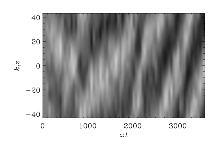
Figure 7: Time-space diagram of ${\overline{u}}_{x}(z,t)$ for Run 7f. $k_{\rm f}/k_{1}=14$, ${\cal R}=3$. Positive values of ${\overline{u}}_{x}$ are shown in light and negative values in dark. Note the migration in the positive $z$-direction.

3.2 Magnetic fields

We now discuss runs where the value of ${\cal R}_{\rm m}$ is large enough to allow dynamo action. A good example is Run 7g where ${\cal R}_{\rm m}=12$. Here the kinematic growth rate of the magnetic field is $\lambda=0.02\omega$. The initial field has grown by a bit more than five orders of magnitude before it reaches saturation, which is when $\omega t\approx\ln 10^{5}/0.02\approx 600$. One clearly sees that at this time the large scale flow becomes strongly suppressed; see Fig. 8, where we have plotted the evolution of kinetic energies contained in various Fourier modes. The normalized magnetic field strength, ${\cal B}$, saturates at a value similar to the normalized velocity, ${\cal U}$. Looking at Table LABEL:T1, it is clear that for all runs with a magnetic field the large scale flow is strongly suppressed, i.e. ${\cal U}_{\rm LS}/{\cal U}$ never exceeds the value $0.1\dots 0.2$.

Figure 8: Evolution of spectral energy in different modes in a lin-log plot. The inset shows the same, but here the ordinate scale is linear. Run 7g.

Figure 9: Power spectra of kinetic (upper panel) and magnetic (lower panel) energies for Run 7g at different times before saturation of the large scale fields (dotted lines) and after saturation (solid lines). Note that after saturation the inverse cascade-type behaviour in velocity is replaced by an inverse cascade-type behaviour of the magnetic field.

Prior to saturation of the magnetic field the kinetic energy spectrum looks like that in Fig. 1, with peaks at both the forcing scale as well as the largest scale of the system; see Fig. 9. (The multiple peaks to the right of the forcing wavenumber come from higher harmonics that are here more pronounced than at higher values of ${\cal R}$; cf. Fig. 1.) However, as the magnetic energy approaches saturation, the kinetic energy becomes suppressed at large scales. Figure 9 shows that, in the saturated state, the kinetic energy spectrum has lost its second peak at $k=k_{1}$. Instead, the magnetic energy spectrum has now attained a shape similar to that of the kinetic energy before saturation. In that sense, the inverse cascade-type behaviour in velocity is now replaced by an inverse cascade-type behaviour of the magnetic field.

Figure 10: Evolution of ${\cal U}$, ${\cal U}_{\rm LS}$, and ${\cal B}$ (upper panel) and ${\cal H}_{\rm K}$, ${\cal H}_{\rm M}$, and $\tilde{\cal H}_{\rm M}$ (lower panel). Run 7g.

In Fig. 10 we have plotted the evolution of ${\cal U}$, ${\cal U}_{\rm LS}$, and ${\cal B}$ (upper panel) together with the relative kinetic and magnetic helicities, ${\cal H}_{\rm K}$ and ${\cal H}_{\rm M}$, as well as the nondimensional length scale related to the magnetic helicity, $\tilde{\cal H}_{\rm M}$ (lower panel). The kinetic helicity is always negative and temporarily enhanced around the time when the magnetic field reaches saturation. We recall that at each instant the forcing has zero helicity, and it is only due to the temporal shift of the forcing pattern that helicity is introduced into the flow.

The magnetic field has positive helicity (Fig. 10). The opposite signs of kinetic and magnetic helicities are in agreement with what is found for helically forced turbulence; see Brandenburg (2001), where the forcing was however chosen to have positive helicity. This led to positive helicity of the flow, so all signs are reversed compared to the present case. Indeed, closer inspection of the power spectrum of the magnetic helicity shows that at small scales the signs of kinetic and magnetic helicities agree. However, because of (approximate) helicity conservation the integrated helicity spectrum has to vanish, which is why at large scales the sign of magnetic helicity is reversed.

4 Conclusions

The present calculations have verified the possibility of the formation of large scale flows from small scale flows lacking parity invariance. These large scale flows tend to be helical and of Beltrami type, as expected from the nature of the anisotropic kinetic alpha (or AKA) effect. The power of the large scale flows tends to be more strongly distributed over several Fourier modes. This is in stark contrast to the magnetic inverse cascade or the dynamo alpha effect which tends to select just one large scale Fourier mode – at least in the case of a fully periodic box; see Brandenburg (2001).

The resulting flows support the possibility of dynamo action once the magnetic Reynolds number exceeds a value typical of non-helical dynamo action. This critical value of the magnetic Reynolds number, based on the wavenumber of the forcing, is around 10. For comparison, in the case of fully helical forcing, the critical dynamo numbers are about ten times smaller; cf. Brandenburg (2001), where the magnetic Reynolds numbers based on the forcing scale need to be divided by $2\pi$ to be compatible with the present work. However, once the magnetic field reaches saturation, it begins to suppress the large scale flow.

In the present work we have adopted the forcing function of Frisch et al. (1987). This has the advantage that we were able to make contact with earlier studies where the AKA effect was also considered numerically. This flow was constructed on purely mathematical grounds in order to demonstrate the very existence of the AKA effect. Other more realistic types of forcing have been proposed by Levina et al. (2000). It is important to extend the present studies to these types of forcing in order to see whether the AKA effect works for broader classes of forcing. However, our present results suggest that the anisotropic kinetic alpha effect should not play a role in astrophysics where the value of ${\cal R}$ is in general large and magnetic fields are usually present. It should be emphasized that in some of the best cases where a large scale velocity pattern emerged (e.g. Run 7f), the large scale flow pattern is never really as pronounced as the large scale magnetic fields that are produced by helical turbulence (cf. Brandenburg 2001).

Finally, we should mention that our results do by no means address the question of whether or not large scale vortices can form astrophysical bodies such as giant planets or accretion discs. Such vortices are long-lived, quasi-stable formations, possibly belonging to the class of solutions studied by Goodman et al. (1987). It it possible that they are formed simply as a matter of suitable initial conditions, but they were also found in simulations of Hawley (1987). This type of solution would be essentially nonlinear, in contrast to solutions of the mean-field equations with AKA effect which are possible already in linear approximation.

Id: paper.tex,v 1.66 2001/06/15 13:31:19 brandenb Exp