Forming stars on a viscous timescale: the key to exponential stellar profiles in disk galaxies?

Abstract

We argue for implementing star formation on a viscous timescale in hydrodynamical simulations of disk galaxy formation and evolution. Modelling two-dimensional isolated disk galaxies with the Bhatnagar-Gross-Krook (BGK) hydrocode, we verify the analytic claim of various authors that if the characteristic timescale for star formation is equal to the viscous timescale in disks, the resulting stellar profile is exponential on several scale lengths whatever the initial gas and dark matter profile. This casts new light on both numerical and semi-analytical disk formation simulations which either (a) commence star formation in an already exponential gaseous disk, (b) begin a disk simulation with conditions known to lead to an exponential, i.e. the collapse of a spherically symmetric nearly uniform sphere of gas in solid body rotation under the assumption of specific angular momentum conservation, or (c) in simulations performed in a hierarchical context, tune their feedback processes to delay disk formation until the dark matter halos are slowly evolving and without much substructure so that the gas has the chance to collapse under conditions known to give exponentials. In such models, star formation follows a Schmidt-like law, which for lack of a suitable timescale, resorts to an efficiency parameter. With star formation prescribed on a viscous timescale however, we find gas and star fractions after $\sim$ 12 Gyr that are consistent with observations without having to invoke any “fudge factor” for star formation. Our results strongly suggest that despite our gap in understanding the exact link between star formation and viscosity, the viscous timescale is indeed the natural timescale for star formation.

1 Introduction

The origin of the exponential radial light profiles in galaxy disks is controversial. The in situ scenario argues for stars forming in an already exponential gaseous disk (Gunn 1982; van der Kruit 1987; Dalcanton, Spergel & Summers 1997; Mo, Mao & White 1998). The viscous scenario, on the other hand, contends that regardless of the initial gas density profile in the disk prior to star formation, the stars will acquire an exponential profile, provided star formation proceeds on a viscous timescale (Silk & Norman 1981; Lin & Pringle 1987; Clarke 1989; Yoshii & Sommer-Larsen 1989; Saio & Yoshii 1990; Olivier, Blumenthal & Primack 1991; Silk 2001; Ferguson & Clarke 2001).

The in situ scenario defers the problem of the origin of exponential stellar light profiles to the origin of the exponential gas distribution. The explanation for such a gas distribution stems from a remark made by Mestel (1963) on the similarity of the specific angular momentum distribution observed in the disks of spirals to that of a uniform sphere in solid body rotation. If specific angular momentum is conserved during the collapse of such a gaseous sphere, the resulting disk naturally retains the sphere’s original angular momentum distribution. Considering the case where this uniform sphere of gas collapses within an isothermal dark halo, Gunn (1982) found that the gas surface density distribution in the final disk would be approximately exponential over three scale lengths.

This simple model is the basis of recent explanations of a host of disk properties. By extending Gunn’s scenario to allow the dark halo to adiabatically respond to the accumulation of baryonic mass in its center, Dalcanton et al. (1997) explained not only the structural properties of present-day disks (e.g. their exponential stellar profiles) but also their dynamical properties (e.g. their rotation curves, the Tully-Fisher relation). Using the Press-Schechter prescription to compute the abundance of virialized halos (Press & Schechter 1974), combined with the prediction from numerical simulations of both the halo dark matter density profiles (Hernquist, 1990; Navarro, Frenk & White 1996) and spin parameters (Barnes & Efstathiou 1987; Warren et al. 1992), these authors also predicted the surface brightness and scale length distributions of present-day disks. Mo, Mao & White (1998), using a similar modelling, extended this study to predict the evolution of disk properties within various cosmological models.

In addition to the simple initial conditions set out by Mestel and Gunn, models built upon the in situ star formation scenario require a recipe for converting gas to stars. In the case of Dalcanton et al. (1997), Mo et al. (1998), and more generally in all semi-analytic models as well as numerical simulations, a Schmidt law, with an efficiency parameter is adopted (see e.g. Kauffmann, White & Guiderdoni 1993; Cole et al. 1994; Somerville & Primack 1999; Katz 1992; Mihos & Hernquist 1994; Steinmetz & Müller 1995; Gerritsen & Icke 1997; Springel 1999). Of course, to imprint the exponential profile on the stars, such a prescription must ignore any process that could significantly redistribute the gas mass and angular momentum in the disk, such as gaseous outflows or viscous flows induced by a turbulent ISM or spiral arms.

Numerous hydrodynamical disk formation simulations have shed light on the in situ theory for the origin of exponential disk profiles. The earliest were N-body plus SPH simulations, first without star formation (Katz & Gunn 1991) and then with stars (Katz 1992). These simulations followed the collapse of an isolated, uniform density perturbation in solid body rotation embedded in an expanding universe. External tidal fields were neglected. Since some small-scale power was added, dark matter and gas clumped prior to the gas dissipating its energy and falling to form a disk. Obviously, the merging of these subclumps involved angular momentum transfer, but apparently the deviation from Mestel and Gunn’s idealized initial conditions was minor and the final gaseous and stellar profiles were well-fit by exponentials. All other simulations starting from similar initial conditions have led to the same conclusion (Vedel, Hellsten & Sommer-Larsen 1994; Steinmetz & Müller 1995; Contardo, Steinmetz & Fritz-von Alvensleben 1998).

In the current paradigm of hierarchical galaxy formation however, one needs to follow the formation of disk galaxies in the context of a more realistic tidal field, for it seems implausible in such a paradigm that all gas destined to settle into a disk originated in a rigidly rotating spherical protocloud which conserved its specific angular momentum not only during the process of protogalactic collapse and settling into centrifugal equilibrium but also throughout the star formation process. Unsurprisingly, hydrodynamical simulations of hierarchical galaxy formation illustrate how nonspherical subclumps of gas and dark matter torque eachother while merging. In fact, in such simulations of only gas and dark matter, there is so much transfer of angular momentum during merging that the disks which form have angular momenta two orders of magnitude lower than what is observed (Navarro & Steinmetz 1997).

To remedy this, attempts have been made to delay the cooling and subsequent collapse of gas in dark halos, so that disks could form late in cosmological simulations when dark matter halos are evolving more slowly and have much less substructure (Weil, Eke & Efstathiou 1998). In these situations, the idealized initial conditions envisioned by Gunn (1982) may be an accurate starting point for disk formation. First attempts at physically motivating such a delay by including feedback mechanisms instead of just switching on cooling in a simulation at a late epoch have been undertaken by Sommer-Larsen, Gelato & Vedel (1999). In their most successful cases, the gas surface densities of their disks are poorly represented by exponentials (their Figure 4). However, resolution in their simulation (between 3303 and 5017 gas particles in a disk) is such that determining a disk scale length is already a difficult task. Hence it may be resolution that prevents these profiles from looking more exponential. At any rate, on the evidence of current numerical simulations, we find it hard to be convinced that all or even most gaseous disks forming in a hierarchical context will acquire an exponential profile.

Rather than trying to fine tune the simulations to obtain idealized initial conditions, it seems more appealing to look for a mechanism that could drive the stellar profile towards an exponential, regardless of the gas profile it starts from. Bearing in mind that star formation and the accompanying complexity of stellar feedback are poorly understood and would be hard to simulate (for obvious resolution issues) even if they were understood, the best that one can do is to model processes which govern star formation on a large scale. With this intention, as an alternative to Katz’s (1992) star formation recipe based on the physics of Jeans instability, we propose to capture the physics that drives star formation by modelling the interstellar medium as a turbulent fluid of colliding, fragmenting and star-forming clouds with energy to drive the turbulence supplied from supernovae, stellar winds, and ionizing radiation from newly born stars. Such turbulence would drive viscous flows.

Therefore, as a start, in this paper, we use numerical hydrodynamical simulations to revisit the hypothesis that star formation occuring on a viscous timescale in galaxy disks yields exponential stellar profiles. Lin & Pringle (1987) explored this question by numerically integrating 1D differential equations, and Yoshii & Sommer-Larsen (1989) confirmed their result by deriving analytical solutions for the star forming viscous disk. Saio & Yoshii (1990) extended these works by including self-gravity. The numerical hydrodynamical approach finds its justification in the fact that, in the future, we want to extend these investigations beyond 1D calculations, and with physics that is difficult to include in an analytic approach (e.g. stellar mass loss, supernovae feedback).

The outline of the paper is as follows: after a discussion of turbulence as a plausible source of viscosity in galaxy disks (section 2) and a description of our numerical approach (section 3), we commence with benchmarking our code to the viscous evolution of a pure gaseous disk without star formation (section 4). Then we proceed to a detailed examination of experiments of star formation in viscous galaxy disks with different initial gas profiles and dark halo rotation curves (section 5). Finally, we discuss our results (section 6).

2 Physical motivation for viscosity

A general consensus among the astrophysical community is that the true kinematic viscosity of the interstellar medium, $\nu$, is much too low to alter the galactic disk structure on a timescale comparable to the age of the universe. It has been argued by various authors (Lynden-Bell and Pringle 1974; Silk and Norman 1981; Lin and Pringle 1987; Yoshii and Sommer-Larsen 1989; Clarke 1989; Olivier et al. 1991; Duschl et al. 2000; Silk 2001) however, that viscous turbulence could drive a non-negligible radial flow of gas in galactic disks.

Turbulence is a consequence of fluid motion, therefore to be maintained it requires an external energy source $E_{ext}$. This energy which arises on large scales, with characteristic velocity $U$ and length $L$, is progressively transferred to smaller and smaller scales by non-linear interactions, until the dissipation scale $L_{dis}$ is reached where molecular processes convert it into heat. It follows from dimensional arguments that $E_{ext}\sim U^{3}/L$. Similarly, one can obtain $L_{dis}\sim(\nu^{3}E_{ext}^{-1})^{1/4}$. As a result,

$$\frac{L}{L_{dis}}={\mathrm{Re}}^{3/4}\,\,,{\mathrm{Re}}=\frac{UL}{\nu}$$ (1)

where ${\mathrm{Re}}$ is the Reynolds number.

Although star formation and/or magnetic fields certainly participate in feeding turbulence, we may suppose that turbulence is driven by differential rotation, (as argued by e.g. Richard and Zahn (1999) for accretion disks), for the following qualitative argument does not change. Typical values for a galactic disk are $L\sim 10^{19}$m (radius of an orbit), $U\sim 10^{5}\rm{m~{}s}^{-1}$ (corresponding azimuthal velocity) and $\nu\sim 10^{-11}\rm{m}^{2}~{}\rm{s}^{-1}$ (we have assumed an average density of $10^{6}\rm{at~{}m}^{-3}$, a temperature of $10^{4}$K and described the gas as elastic spheres of diameter $10^{-10}$m). Combined together, these numbers lead to ${\mathrm{Re}}\sim 10^{35}$. This extremely high Reynolds number means that in order to fully resolve our problem numerically in 3D, we should have about $10^{79}$ grid points (see eq. 1), whereas state-of-the-art super computers can handle $10^{10}$ at most. Therefore, the only way around this problem is to somehow model what happens on subgrid scales and numerically resolve the properties of the flow on large scales.

As first noted by Boussinesq (1870), it seems that to first order and on macroscopic scales the net effect of turbulence is simply to turn the real fluid into a more viscous one. This can be schematically understood as follows: the Reynolds number of a turbulent fluid is so high that any perturbation in the smooth flow produces eddies which dissipate energy until the flow reaches a critical, lower Reynolds number $\rm{Re}_{c}$, corresponding to the onset of turbulence. If more eddies are produced, the effective viscosity becomes too high, cutting off the production of eddies. On the other hand, if not enough eddies are produced, then the flow still exhibits a tendency to produce turbulence. Laboratory flow values for critical Reynolds numbers are on the order of $\rm{Re}_{c}\sim 10-10^{3}$ (see for example Richard and Zahn 1999), so that one can solve the Navier–Stokes problem with this critical Reynolds number and hope that it is enough to obtain a good description of the properties of the flow on macroscopic scales.

Our goal here is not to derive a mathematically rigorous formulation of hydrodynamic turbulence in galactic disks but to suggest that there exist strong physical arguments in favor of describing the behaviour of the gas flow on large scales by simply solving a Navier–Stokes problem with a smaller Reynolds number, namely the critical Reynold’s number, $\rm{Re}_{c}\sim 10-10^{3}$.

3 Numerical approach

We perform numerical hydrodynamical simulations in 2D with the BGK (Bhatnagar-Gross-Krook) code (Prendergast and Xu 1993, Slyz and Prendergast 1999). This is a scheme based on gas-kinetic considerations, meaning the code solves for the time evolution of a gas distribution function, $f({\vec{x}},{\vec{u}},t)$, in phase space. Fluxes are computed from velocity moments of $f$. $f$ evolves in time according to an approximation to the collisional Boltzmann equation, namely the BGK equation: $\frac{Df}{Dt}=\frac{g-f}{\tau}$ where $\frac{D}{Dt}$ is a time rate of change along the trajectory of a single particle moving freely in phase space under the action of a smoothly varying gravitational field and where $\frac{g-f}{\tau}$ models the effects of collisions. Here $g$ is a local equilibrium distribution, i.e. the Maxwell-Boltzmann distribution function, having the same mass, momentum and energy densities as $f$, and $\tau$ is a relaxation time, which can be as small as the mean time between collisions of a particle in the gas (Bhatnagar, Gross & Krook 1954). The underlying hypothesis of the BGK model is that there is a relaxation process in which collisions tend to reshuffle the particles defining the true distribution function, $f({{\vec{x}}},{{\vec{u}}},t)$ to $g({{\vec{x}}},{{\vec{u}}},t)$, while conserving the total mass, momentum and energy. This conservation requires that the moments of the BGK collision term must vanish. $f$’s relaxation to the equilibrium state $g$ is dissipative and hence is accompanied by an increase in entropy. It is nontrivial that the BGK scheme captures this physics. Many schemes have to invoke an “entropy fix” usually in the form of artificial viscosity to mimic an entropy increase and eliminate unphysical numerical phenomena such as rarefaction shocks.

Together with the criteria of vanishing moments of the collision term, a numerical solution of the formal integral solution (eq. 2 below) of the BGK equation comprises the BGK scheme. Given initial conditions $f=f_{0}$ at $t=t_{0}=0$, the solution to the BGK equation contains two terms: an integral over the past history of $g$ and a term representing relaxation from an initial state, $f_{0}$ on a timescale $\tau$.

$$f({\vec{x}}_{f},{\vec{u}},t)=\frac{1}{\tau}\int^{t}_{0}g({{\vec{x}}}^{{}^{\prime}},{{\vec{u}}}^{{}^{\prime}},t^{{}^{\prime}})e^{-(t-t^{{}^{\prime}})/\tau}\,dt^{{}^{\prime}}+$$

$$e^{-t/\tau}\,f_{0}({\vec{x}}_{f}-{\vec{u}}t,{\vec{u}},t_{0})$$ (2)

Here ${\vec{x}}^{{}^{\prime}}$ and ${\vec{u}}^{{}^{\prime}}$ in the arguments of $g$ are points along a gas particle’s trajectory in phase space with the final conditions ${\vec{x}}^{{}^{\prime}}={\vec{x}}_{f}$ and ${\vec{u}}^{{}^{\prime}}={\vec{u}}$ at $t^{{}^{\prime}}=t$. When fluxes are eventually computed at ${\vec{x}}_{f}$, $f({\vec{x}}_{f},{\vec{u}},t)$ is integrated over the full and continuous range of velocities, ${\vec{u}}$, from $-\infty$ to $+\infty$. Therefore fluxes computed from the true distribution function $f({\vec{x}}_{f},{\vec{u}},t)$ arise by a weighted integration of the equilibrium distribution function $g({{\vec{x}}^{{}^{\prime}}},{{\vec{u}}^{{}^{\prime}}},t^{{}^{\prime}})$ not just over one trajectory but over all possible trajectories (in 6-dimensional phase space) which arrive at (${\vec{x}}_{f},t$). A detailed description of the numerical procedure in the BGK scheme for the 2D Cartesian case is given in Xu (1998).

By evolving $f$ through an equation which accounts for particle collisions, the fundamental mechanism for generating dissipation in gas flow, the BGK scheme gives fluxes which carry both advective and dissipative terms. This means that for viscous problems no modification to the BGK flux expressions from their form for non-viscous problems is necessary. Furthermore there is no need for viscous source terms. More than this, unlike the earlier gas-kinetic scheme used in astrophysics, namely the beam scheme (Sanders and Prendergast 1974), which also carried dissipation in its flux expressions, the BGK scheme is dissipative in a realistic way. Where the beam scheme arbitrarily chooses the form of $f$ at the beginning of each updating time step and evolves it through the collisionless Boltzmann equation, the BGK scheme solves for the time evolution of $f$ throughout an updating time step using a model of the collisional Boltzmann equation. If the gas happened to be in disequilibrium at the beginning of the updating time step, the beam scheme cannot readjust the gas properly to equilibrium because it evolves $f$ through the collisionless Boltzmann equation which is simply missing the adjusting mechanism provided by collisions.

Also by assuming instantaneous relaxation back to the chosen form for $f$ at the beginning of an updating time step, the beam scheme endows the gas with a mean collision time equivalent to the updating time step. Collisions in the BGK scheme on the other hand are active throughout the updating time step and for hydrodynamical applications the BGK scheme demands that the collision time is much smaller than the updating time step. Since dissipation parameters are proportional to the collision time, $\tau$, e.g. the dynamical viscosity $\eta=\tau p$, and the heat conduction coefficient $\kappa=\tau\frac{K+5}{2}\frac{pk}{m}$ (where $p$, $k$, $m$ are the gas pressure, Boltzmann constant, and particle mass respectively and $K=\frac{-3\gamma+5}{\gamma-1}$ where $\gamma$ is the ratio of specific heats, $\frac{c_{p}}{c_{v}}$), we easily see that an overestimation of the collision time will lead to a very diffusive scheme.

The BGK code has been extensively tested on standard 1D and 2D test cases of discontinuous nonequilibrium flow with features ranging from cavitation (Roe test) to the collision of strong shocks (Woodward-Collela test) (see Xu 1998 for a review). At shocks and contact discontinuities the code behaves as well as the best high resolution codes which do not employ regridding in the neighborhood of a shock front and it gives better results at rarefaction waves. Because the BGK scheme naturally satisfies the entropy condition, it never requires an entropy fix when it encounters strong rarefaction waves (cf. the Sjögreen test). Tests of the BGK schemes ability to solve the Navier-Stokes equations in smooth flow regions include the Kolmogorov and laminar boundary layer problem (Xu and Prendergast 1994). Tests of the BGK scheme in an external gravitational potential show the long-term stability of the scheme and its convergence to the equilibrium solution (Slyz & Prendergast 1999).

3.1 Quantifying Viscosity in BGK

As already mentioned in the previous section, on a microscopic level dissipative parameters are directly related to the collision time of the gas, $\tau$. Like other finite volume schemes, the BGK scheme follows the mass, momentum and energy densities within cells on an Eulerian grid. For the flux computation, the BGK scheme solves for $f$ in the neighborhood of the boundary of each computational cell and for a short time (given by the usual CFL (Courant-Friedrichs-Lewy) condition). Hence at each time step and at each cell boundary, it is possible to solve the BGK equation with the collision time $\tau$ which is appropriate to the local fluid properties. For example, since gas kinetic theory gives a dependence of collision time on gas density $\rho$ and temperature $T$, an expression for $\tau$ may be written as $\tau=\frac{{\cal C}_{1}}{\rho\sqrt{T}}$ where ${\cal C}_{1}$ is a proportionality constant which is chosen according to the desired Reynolds number of the problem. (${\cal C}_{1}=(UL/Re)(\rho^{2}/\sqrt{\lambda}p)$ where U and L are characteristic velocity and length scales, $\lambda=\frac{m}{2kT}$ where $T$ is the gas temperature, $p$ is the gas pressure, and $Re$ is the Reynolds number.) If we wish to do a problem with constant kinematic viscosity for the case where the Reynolds number is equal to the critical Reynolds number, $Re_{c}$, and an isothermal gas, then we set $\tau$ to have a constant value, $\tau=\frac{2\lambda UL}{Re_{c}}$. Once $\tau$ is known, we can write an expression for the real physical kinematic viscosity coefficient $\nu=\tau\frac{p}{\rho}$.

For problems in which the gas flow has discontinuities, the collision time $\tau$ serves an additional purpose. If the grid is not fine enough to resolve a discontinuity, then artificial dissipation must be added to broaden the discontinuity so that it is at least one grid cell thick. Because viscosity and heat conductivity are proportional to $\tau$, the BGK scheme broadens shocks by enlarging $\tau$ at the location of the discontinuities. The expression for the collision time in the BGK scheme therefore contains another term in addition to the real physical collision time. The second term is chosen in such a way that shocks in the flow span at least one grid cell. In one-dimensional Cartesian coordinates this second term is:

$${\cal C}_{2}\frac{\arrowvert p_{l}-p_{r}\arrowvert}{(p_{l}+p_{r})}.$$ (3)

The subscript $l\hskip 3.00003pt(r)$ denotes quantities interpolated from the left (right) side of the cell interface at which we compute the collision time $\tau$, and $p$ is the gas pressure.

This second term tunes the amount of artificial dissipation in the scheme. The notable difference between how the BGK scheme inputs artificial dissipation and how other schemes input artificial dissipation is that the BGK scheme puts it in exactly as if it were real dissipation corresponding to the numerically necessary value for $\tau$. We again emphasize that neither the artificial dissipation nor the physical dissipation enter the scheme as a source term. When the second term (eq. 3) in the collision time dominates, the order of the scheme is reduced and the true distribution function $f$ is determined more by the initial distribution function $f_{0}$ than by the integral over $g$ (eq. 2). For smooth flow however, such as is encountered in the viscous evolution of a galactic disk in an axisymmetric gravitational potential, $C_{2}$ may be set to zero and the BGK scheme evolves the gas with its true physical dissipation parameters, as long as the grid resolution corresponding to the desired Reynolds number of the problem is achieved.

Even when $C_{2}$ is set to zero, in addition to the (explicit) real physical viscosity in the scheme (controlled by the collision time) there is an inevitable numerical viscosity, dependent on the grid spacing: the coarser the grid, the larger this numerical viscosity. The origin of this viscosity is that the scheme forgets everything except cell averages at the end of each time step. A consequence of this is that when one does a resolution study of the viscous evolution of a gaseous disk, the flow properties on a 207 X 207 grid quantitatively match those on the 85 X 85 grid only when one runs the problem on the finer grid with larger $\tau$.

Figure 1: Early viscous evolution (first 2.28 Gyr) of a disk of pure gas initially in inviscid centrifugal equilibrium ($v_{R}=0$) in a fixed gravitational potential. Coding for the different curves is given in the bottom panel of the figure.

4 Viscous Evolution of a Disk of Pure Gas

Before testing the hypothesis that $t_{\star}\sim t_{visc}$ gives exponential stellar profiles, we check how closely the BGK hydrocode reproduces our analytic predictions for the steady state viscous evolution of a gas without star formation. The interest of performing such a computation is obvious: it allows us to measure the true viscosity of the code as well as its ability to capture the Navier-Stokes solution for a compressible viscous fluid evolving in a fixed gravitational field for the case where the shear flow is highly supersonic (Mach $\approx$ 20) throughout most of the disk. Earlier tests of BGK’s ability to give Navier-Stokes solutions were only for subsonic shear flows (Mach $\approx$ .5 for the laminar boundary layer problem; Mach $\approx$ .8 for the decaying sinuisoidal wave problem) (Xu and Prendergast 1994).

We initialize the gas in a fixed dark halo with gravitational potential:

$$\Phi(r)=\frac{1}{2}{{\rm v_{0}}}^{2}{\rm ln}({{\rm r_{0}}}^{2}+{\rm r}^{2})$$ (4)

where $v_{0}=220$ km/s and $r_{0}=2.56$ kpc. We consider two cases: the case where the gas is initially in inviscid centrifugal equilibrium ($v_{R}=0$), and the case where the gas is in centrifugal equilibrium but the initial radial velocity profile is derived from the Navier-Stokes equations (instead of from Euler’s equations) given our choice of initial gas profile (see Appendix A). We neglect self-gravity and assume constant kinematic viscosity, $\nu$, and uniform temperature at all times ($T\approx 10^{4}$ K). We comment more on the astrophysical motivation behind our choice of initialization in section 5.1.

To obtain a constant $\nu$ in the computation, the collision time $\tau$ in the BGK scheme is set to $\frac{2\lambda UL}{Re_{c}}$ (see discussion in section 3.1) where $U=220$ km/s, $L=20$ kpc, $Re_{c}\approx 750$. The computation is performed on a 207 X 207 Cartesian grid and we follow the flow for about 12 Gyr. We would like to point out that in order to preserve the cylindrical symmetry of the flow on such a grid we had to use the high order limiter described in Huynh (1995). We specify boundary conditions in detail in section 5.1 below.

Figure 2: Same run as in fig. 1 but with the results for the evolution shown up to 11.84 Gyr. The steady-state analytic predictions (asterices) are compared to the BGK numerical results (thin solid curves and empty circles).

Figure 3: Early viscous evolution (first 2.28 Gyr) of a disk of pure gas in a fixed gravitational potential. This time the initial radial velocity is set to the velocity profile given by the solution to the Navier-Stokes equation corresponding to the initial density profile (see Appendix A for details). Coding for the different curves is given in the bottom panel of the figure.

Figure 4: Same run as in fig. 3 but with the results for the evolution shown up to 11.84 Gyr. The steady-state analytic predictions (asterices) are compared to the BGK numerical results (thin solid curves and empty circles).

In figures 1 and 2 we plot the code’s results for the time evolution of the gas surface density, $\Sigma_{g}$, the radial velocity, $v_{R}$, and the ratio of the circular velocity at time $t$ to its initial value, $\frac{v_{c}(t)}{v_{c}(0)}$ starting with an inviscid equilibrium solution (i.e. with $v_{R}=0$ initially) and a nearly uniform mass density distribution. In figures 3 and 4 we show a similar time evolution of these quantities but in this case we start from an initial $v_{R}$ consistent with the Navier-Stokes solution corresponding to the initial density profile we choose . Overplotted are the analytic predictions. These predictions are obtained by solving the Navier-Stokes equations for a compressible viscous fluid in cylindrical coordinates along with the equation of continuity:

$$\Sigma_{g}\left(v_{R}\frac{dv_{R}}{dr}-\frac{v_{C}^{2}}{r}\right) = -\frac{dp}{dr}-\frac{d\Phi}{dr}$$ (5)

$$+ \left(\xi+\frac{4}{3}\eta\right)\left(\frac{d^{2}v_{R}}{dr^{2}}+\frac{1}{r}\frac{dv_{R}}{dr}-\frac{v_{R}}{r^{2}}\right)$$

$$+ 2\frac{d\eta}{dr}\frac{dv_{R}}{dr}$$

$$+ \left(\frac{d\xi}{dr}-\frac{2}{3}\frac{d\eta}{dr}\right)\left(\frac{dv_{R}}{dr}+\frac{v_{R}}{r}\right)$$

$$\Sigma_{g}v_{R}\left(\frac{dv_{C}}{dr}+\frac{v_{C}}{r}\right) = \eta\left(\frac{d^{2}v_{C}}{dr^{2}}+\frac{1}{r}\frac{dv_{C}}{dr}-\frac{v_{C}}{r^{2}}\right)$$ (6)

$$+ \frac{d\eta}{dr}\left(\frac{dv_{C}}{dr}-\frac{v_{C}}{r}\right)$$

$$\Sigma_{g}\left(\frac{dv_{R}}{dr}+\frac{v_{R}}{r}\right) = -\frac{d\Sigma_{g}}{dr}v_{R}$$ (7)

The fundamental assumption that permits the analytic calculation is that the circular velocity $v_{C}$ remains unchanged, and therefore one only needs to use the second Navier-Stokes equation (eq. 6) and the continuity equation (eq. 7). However, this assumption can be tested a posteriori, when the solutions for density $\Sigma_{g}$ and radial velocity $v_{R}$ have been computed. If one plugs these solutions in the first Navier-Stokes equation (eq. 5), it is easy to check that, to second order in viscosity it is satisfied. The analytic steady state solution of the system therefore is:

$$v_{C}(r) = v_{0}\frac{r}{(r_{0}^{2}+r^{2})^{1/2}}$$ (8)

$$v_{R}(r) = -\nu\frac{r}{r_{0}^{2}+r^{2}}$$ (9)

$$\Sigma_{g}(r) = \Sigma_{g}(0)\frac{r_{0}^{2}+r^{2}}{r^{2}}$$ (10)

One important remark is that this set of solutions depends only on the shape of $v_{C}$ through the parameter $r_{0}$. Therefore, provided that the gravitational potential is fixed, the radial inflow of gas ($v_{R}$ is always negative) after a certain time should be the same whatever the initial conditions we choose for the gas. Unfortunately, things are more complicated for the density profile because the analytic solution for $\Sigma_{g}(r)$ diverges for $r=0$. However, there is an obvious comment that we can make: the steady state density profile is not exponential, which implies that it is the interplay between viscosity and star formation that must be responsible for turning stellar profiles into exponentials in the viscous scenario.

The first thing to notice in figures 1, 2, 3 and 4 is that the BGK scheme drives the gas towards a radial velocity profile which is in excellent agreement with the predicted analytic profile, independent of the initial profile for $v_{R}$. We will show in section 5.4 that this also holds when we start from a different initial density profile and/or a different gravitational potential profile, again in perfect agreement with the analytic expectations. The situation for the density profile is different because to obtain a good match to the analytic fit for a density profile which diverges like $r^{-2}$ in $r=0$, one requires an infinite amount of time and mass. As we can only run the computation for a finite amount of time and handle finite numbers, we obviously cannot achieve the steady state density distribution, even though one clearly sees that the gas will perpetually pile up in the center of the simulated disk. We also point out that the circular velocity of the gas, $v_{C}$, remains unchanged up to a tenth of a percent throughout almost all of the disk, which numerically confirms the validity of our analytic assumption that it is constant in time. Finally, although we do not show the results in this paper, we have also verified that decreasing $Re_{c}$, which is equivalent to increasing $\nu$, results in the gas showing a similar radial flow in shape, but with a higher normalisation.

The success of BGK in giving viscous radial flows on the order of 1 km/s in a disk rotating differentially at 220 km/s is remarkable. It is a technical success which is necessary for studying star formation on a viscous time scale in disks since chemical evolution models (Lacey and Fall 1985, Clarke 1989) find that radial flows on that order can explain the radial distribution of metals in disk galaxies.

5 Star formation in viscous galaxy disks

5.1 Initialization and Boundary Conditions

For our simulations with star formation, the initialization is similar to the initialization of the purely gaseous disk described in section 4. Here we elaborate on our initial and boundary conditions, and discuss our motivation for choosing this problem set-up. We initialize our gas to be in a fixed dark matter halo and we model the dark matter halo with the logarithmic potential defined by equation 4. We choose this form for $\Phi$ because of its simplicity which allows us to perform analytical computations for comparison. Furthermore this potential has the property that the rotation curve corresponding to it becomes asymptotically flat with velocity $v_{0}$ at large radii as is observed for many spiral galaxies. All the results presented in this paper are from runs with $v_{0}$ = 220 km/s. The total mass of the dark halo is chosen to be $10^{12}{\rm M}_{\odot}$ and that of the gaseous disk $5\%$ of the dark matter, i.e. $5\times 10^{10}{\rm M}_{\odot}$. Given that the gas is a small fraction of the dark matter, we neglect its self-gravity and assume that it evolves in the fixed potential created by the dark matter.

We perform our simulations with an isothermal equation of state, meaning that we assume that at the end of each iteration the gas instantanesouly cools to $\approx 10^{4}{\rm K}$. We choose this temperature because it is the lowest achievable from HI line cooling alone. Below that temperature we would have to worry about the formation of molecular hydrogen, which we neglect because we do not have the necessary resolution to follow the formation and fragmentation of molecular clouds in the context of an entire galaxy. Accounting for a molecular component would also require us to follow an atomic and molecular fluid simultaneously, which would considerably increase the complexity and computational cost of the simulation and therefore is beyond the scope of this paper. For a $\gamma=\frac{5}{3}$ gas a temperature of $\approx 10^{4}{\rm K}$ corresponds to a sound speed of $\approx 10$ km/s.

Since we want to initialize the gas with self-consistent viscous initial conditions, we set the radial flow to be given by the profile derived from the Navier-Stokes equations (see Appendix A), assuming centrifugal equilibrium for a particular initial gas density profile in a potential $\Phi$ with a core radius $r_{0}$ (eq. 4). Indeed, due to the observed thinness of stellar disks in nature (scale height $\approx$ 200 pc), and the difficulty of dissipating stellar motions perpendicular to the galactic plane, it seems reasonable to assume as an initial condition for the radial velocity that the gas collapsing to a disk in the dark matter halo was in approximate centrifugal equilibrium before it started forming stars.

We choose 20 kpc for the disk radius of our simulations because based on observations of OB stars (Chromey 1978) and of HII regions (Fich and Blitz 1984), the stellar disk of our own Galaxy seems to have an outer cutoff around this value. Our computations are performed on a 207 by 207 evenly spaced Cartesian grid, so that for a disk with radius 20 kpc the cell size is about 200 pc per side. Again, we emphasize that we are not trying to resolve star formation on a small scale. We are trying to model the first order effect of turbulence, a phenomenon which might govern star formation on a large scale. We run each simulation for about 12 Gyr. On a grid of 207 X 207 this takes approximately 50,000 iterations and requires about 11 hours of CPU time per processor on an Origin 2000 with four r12k processors working in parallel.

We investigate the case where the kinematic viscosity, $\nu$ is constant because it is a simple case for which we can compute analytic solutions for the radial velocity exactly and compare them to the results from our hydrodynamical simulation. As already described in section 4, to achieve a constant $\nu$, we set the collision time $\tau=\frac{2\lambda UL}{Re_{c}}$. We again take $U=220$ km/s, $L=20$ kpc, ${\rm Re_{c}}=750$ and $\lambda=\frac{m}{2kT}$ with $T\approx 10^{4}$K. We underscore that our choice for $\nu$ is motivated by our intention to model a disk with a critical Reynolds number $\approx$ 750, because in this way as discussed in section 2, we model the lowest order effect turbulence has on a flow, namely to turn it into a more viscous fluid with $Re=Re_{c}$ .

Our boundary conditions are as follows. Outside of a radius of $R_{\rm disk}$ on our 2D Cartesian grid, we keep two “rings” of ghost cells, each “ring” being one cell thick. Beyond these ghost cells we do not follow the evolution of the gas. In this way we have carved a circular grid out of the square cartesian grid. At the end of each updating time step of the code, we replace the values of the velocities in the ghost cells with the values of the closest active ring of cells (these for which the evolution is computed). This means that we are actually performing a constant radial extrapolation to reset the values of all the macroscopic quantities (density, momentum and energy) in the ghost cells. Basically, this is an implementation of “outflow” boundary conditions, where the active region dictates the behaviour of the flow inside the boundaries. Nevertheless, despite this a priori free boundary condition, we find that the mass flow across the outer boundaries of the grid is under control. At most our boundary conditions lead to a maximal loss/gain in total mass on the grid of $1.7\%$ (see tables 1 and 2). This was to be expected, since analytic calculations (eq. 9 and fig. 4) show that for the critical Reynolds number we are using, the outer radial flow should eventually settle around a value smaller than $0.5$ km/s. In the future, it will be interesting to investigate the effect of infall onto the disk and for this we will obviously have to alter these boundary conditions.

5.2 The star formation timescale

Figure 5: Comparison of the final stellar profiles (after $\approx$ 12 Gyr of evolution) for different values of the star formation timescale to the viscous timescale, $\beta$. The initial radial velocity profile is derived from the Navier-Stokes equation for the corresponding initial density profile, $\Sigma_{g}^{i}=\Sigma_{0}/(1+({\frac{r}{r_{p}}})^{2})$ where $r_{p}=78$ kpc, $\Sigma_{0}=41.08{\rm M}_{\odot}/{\rm pc^{2}}$, and $r_{0}=2.56$ kpc in the gravitational potential (see Appendix A for details).

The first point that we wish to verify is that if star formation proceeds on the same timescale as the viscous redistribution of mass and angular momentum in disk galaxies then the stars attain an exponential density profile. We therefore define the viscous timescale, $t_{\rm visc}$, by $r/{v_{R}}$. This estimates the time it takes a disk annulus to move a radial distance $r$. Our star formation law then simply reads:

$$\frac{d\Sigma_{\star}}{dt}(r,t)=\frac{\Sigma_{g}(r,t)}{t_{\star}}=\Sigma_{\rm SFR}(r,t)$$ (11)

where, unless explicitly specified, $t_{\star}=t_{\rm visc}$. In the steady state, $t_{\rm visc}=(r_{0}^{2}+r^{2})/{\nu}$, so that at large radii the assumption of a constant kinematic viscosity corresponds to a star formation rate per unit area of $\Sigma_{\rm SFR}\propto\Sigma_{g}/r^{2}$. This $\Sigma_{\rm SFR}$ corresponds to a Schmidt law with $n=1$ modulated by $r^{-2}$ which means that the star formation rate at large radii is very slow. Note that since $v_{R}$ varies with space and time until the steady state is achieved, after which point it only varies with space, $t_{\rm visc}$ (and hence $t_{\star}$) has a similar behaviour. We assume, as do Lin & Pringle (1987), that once the stars form, they are frozen out of the viscous evolution and simply move on circular orbits with a velocity given by the rotation curve at the location at which they form. Hence we neglect any process that might give the stars a velocity dispersion after they have formed. As a result of these assumptions, the implementation of star formation in the simulation only introduces a sink term, $-\Sigma_{g}(r,t)/t_{\star}$, in the continuity equation 7.

Figure 6: Fitting residuals for $\beta=1$ case (top) and $\beta=10$ case (bottom). Thin solid lines are the residuals for the best power law fit to the stellar profile and the long dashed lines are the residuals for the best exponential fit. The fit is done only over the radii enclosed within the vertical short-dashed lines. The scale length of the exponential fit, $r_{s}$, and the exponent of the power-law fit, $\alpha_{p}$, are given on each panel.

Figure 7: Time evolution of gas density (uppermost panels), radial velocity (second panels from top), tangential velocity (third panels from top) and stellar density (bottom panels) for $\beta$ = .1 (left panels), i.e. a simulation where star formation takes place quickly compared to the viscous timescale, $\beta$ = 1 (middle panels), i.e. a simulation where star formation occurs on a viscous timescale and $\beta$ = 10 (right panels), i.e. a simulation where star formation is much slower than the viscous timescale.

We perform a set of three runs with varying star formation timescales. Using Lin and Pringle’s notation of $\beta=t_{\star}/t_{visc}$, we run the code for the same three cases that these authors considered: $\beta=.1,1,10$. The initial gas density is $\Sigma_{g}^{i}=\Sigma_{0}/(1+({\frac{r}{r_{p}}})^{2})$ where $r_{p}=78$ kpc, $\Sigma_{0}=41.08{\rm M}_{\odot}/{\rm pc^{2}}$, and $r_{0}=2.56$ kpc in the gravitational potential. Results are shown in figures 5, 6 and 7.

Figures 5 and 6 show a comparison of the stellar profiles we obtain after about 12 Gyr for these three different values of $\beta$. Just as Lin and Pringle claimed, we find that the initial gas profile is nearly frozen into the stellar profile for small $\beta$ because star formation is so rapid that almost no viscous redistribution of matter can take place before the stars form. Furthermore, as illustrated in the left panels of figure 7 which show the time evolution of the gas density, radial velocity, and stellar density (top to bottom), almost all the gas is converted into stars by 12 Gyr (more than 98 %). This is inconsistent with present-day spirals like the Milky-Way which still have a supply of gas of order 15 % (Prantzos & Aubert, 1995) to fuel ongoing star formation in their disks.

At the other extreme is the case of large $\beta$. Here too much viscous evolution occurs and the resulting stellar profile is more a power law than an exponential (see bottom panel of figure 6). Furthermore, the amount of stars formed during 12 Gyr is negligible (a few %), again in conflict with observations for Milky-Way type spirals which should have formed between 80 and 90 % of their stars.

Only the $\beta$ = 1 case, i.e. the case where stars form on the viscous timescale, gives both approximately an exponential stellar profile (see residuals in top panel of figure 6) and a stellar density which is in better agreement with Milky Way values. The stellar density is still low for this simulation with only about 40 % of stars formed, but this number depends sensitively on the steepness of the initial gas profile (see table 1 and 2). If we use a reasonably steeper (and probably more realistic) initial profile we can bring the amount of stars formed in perfect agreement with the observations, e.g. for the case where $\Sigma_{g}^{i}=\Sigma_{0}/(1+({\frac{r}{r_{p}}})^{4})$, $r_{p}$ = 5.12 kpc, and $r_{0}$ = 1.92 or 2.56 kpc, about 80 % of the disk’s gas is turned into stars after $\approx$ 12 Gyr (see section 5.4). Looking at the lowest middle panel of figure 7, we also see that after about 6 Gyr (9th thin solid curve in the bottom middle panel, the first one being the lowest), the final exponential profile is more or less established in the sense that there is little evolution in its scale length thereafter: the regularly spaced (in time) curves are much closer to one another than they are at earlier times, and their slope is not changing noticeably. The bottom panels of figure 7 lead to the general statement that the evolution of the stellar profile proceeds much more quickly at early times than at later times because the gas content is higher and the radial flows are generally faster in the beginning of the simulation.

In their models of star formation in a viscous disk Firmani, Hernandez & Gallagher (1996) also claim that there appear to be two distinct phases of star formation, the first corresponding to a stage of significant viscous mass and angular momentum redistribution, and the second corresponding to a stage where star formation has reduced the amount of gas in the disk to the point that viscous evolution is very slow and star formation proceeds slowly with an unchanging radial velocity profile for the gas. We remark that interpreting this as two distinct phases of star formation must be done cautiously because Firmani et al. (1996) initially take their gaseous disk to be in inviscid centrifugal equilibrium, so that when they begin to follow the disk evolution with equations of motion which include viscosity, the gas first tries to find a (non-existent) equilibrium for the viscous case and this causes a lot of initial mass and angular momentum redistribution. For instance, comparing our figures 1 and 3, we clearly see that the steady state for the radial velocity is reached much earlier when we start from an initial radial velocity in agreement with the Navier-Stokes solution corresponding to the initial density profile (middle panel of fig 3) than when we start from the inviscid equilibrium solution (middle panel of fig 1). We also note that, whatever the initial conditions, the time taken to reach the steady state is quite short ($\approx$ 2 Gyr for the longest initial inviscid equilibrium case) compared to the duration of the whole simulation (about 12 Gyr).

Figure 8: Comparison of stellar and gas profiles after 12 Gyr for varying initial gas profiles. From top to bottom the initial gas profile is $\Sigma_{g}^{i}=\Sigma_{0}e^{-\frac{r}{r_{e}}}$, $\Sigma_{g}^{i}=\Sigma_{0}/(1+({\frac{r}{r_{p}}})^{2})$, $\Sigma_{g}^{i}=\Sigma_{0}/(1+({\frac{r}{r_{p}}})^{2})$, and $\Sigma_{g}^{i}=\Sigma_{0}/(1+({\frac{r}{r_{p}}})^{4})$. The values of the parameters $\Sigma_{0}$, $r_{e}$, and $r_{p}$ are given in table 1. The parameters defining the gravitational potential are the same for each of these runs, namely $r_{0}$ = 2.56 kpc and $v_{0}$ = 220 km/s.

Since there is yet no absolutely convincing explanation for an equality between the viscous and star formation timescales, it is worthwhile to explore how much leeway there is in the equivalence. Saio & Yoshii (1990) explored the cases where $\beta$ is .5 and 2, as opposed to an order of magnitude greater or smaller than $\beta=$1. They find the $\beta=.5$ case to yield a profile close to the pure exponential disk (van der Kruit 1987) and the $\beta=2$ case to yield a disk with a pronounced bulge and disk. They concluded that the star formation timescale does not have to exactly equal the viscous timescale to produce an exponential stellar profile. Although we do not show results in this paper, we have run simulations with different $\beta$ and confirm that provided it does not differ from unity by more than a factor 2, we get exponential profiles of a similar quality as those presented here.

	Initial Parameters
Profile	$\Sigma_{0}$	$r_{p}$	$r_{e}$	$r_{s}$	$r_{H}$	PL	stars	gas	mass	$\Sigma_{*}$ at $R_{\odot}$	$\Sigma_{g}$ at $R_{\odot}$	$\Sigma_{g}$ at $R_{\odot}$
	(${\rm M}_{\odot}/{\rm pc^{2}}$)	(kpc)	(kpc)	(kpc)	(kpc)	fit			loss	(${\rm M}_{\odot}/{\rm pc^{2}}$)	(${\rm M}_{\odot}/{\rm pc^{2}}$)	(${\rm M}_{\odot}/{\rm pc^{2}}$)
PL, $\alpha_{p}=2$	41.1	78.	–	8.15	13.3	-1.05	41.4	59.6	+1.05	23.8	16.8	40.6
EXP	3537.	–	1.5	1.33	2.52	-4.16	94.3	5.7	-.004	7.5	5.0	11.6
PL, $\alpha_{p}=2$	586.9	2.56	–	3.29	6.62	-2.78	69.5	31.4	+.84	28.4	19.6	40.6
PL, $\alpha_{p}=2$	217.3	5.12	–	3.64	8.6	-2.41	60.8	41.0	+1.7	31.9	25.1	57.1
PL, $\alpha_{p}=4$	115.2	10.2	–	3.47	5.06	-2.85	59.6	41.5	+1.1	45.2	31.8	77.2

Table 1: Results from runs all having the same rotation curve ($v_{0}=220$ km/s and $r_{0}=2.56$ kpc) but different initial gas profiles (PL stands for power law with exponent $\alpha_{p}$, and EXP stands for exponential. See text for more details). Column ṔL fitćontains exponents from the best power law fit to the final stellar profile; the following column gives the percentage of initial gas that has been turned into stars after 12 Gyr. From left to right, the next columns give values for the percentage of gas left after 12 Gyr, the percentage of mass lost (or gained) from the grid after 12 Gyr, the stellar density at the solar radius after 12 Gyr, the final gas density at the solar radius, and the initial gas density at the solar radius.

5.3 Dependence on initial gas profile

The next step is to check the robustness of the $t_{\star}\sim t_{visc}$ hypothesis to varying initial conditions. With this intention, we perform numerical experiments, keeping the rotation curve fixed ($v_{0}=220$ km/s and $r_{0}=2.56$ kpc) while varying the initial gas profile. We have tried the following two profiles: $\Sigma_{g}^{i}(r)=\Sigma_{0}e^{-\frac{r}{r_{e}}}$ and $\Sigma_{g}^{i}(r)=\Sigma_{0}/(1+({\frac{r}{r_{p}}})^{\alpha_{p}})$ where $\Sigma_{0}$ is a constant, $r_{e}$ and $r_{p}$ are the scale lengths of the exponential and power law profile respectively and $\alpha_{p}$ is either $2$ or $4$. For each of the runs with rotation curve prescribed by $v_{0}=220$ km/s and $r_{0}=2.56$ kpc, Table  1 presents the values for $\Sigma_{0}$, $r_{p}$, $r_{e}$ the stellar exponential scale length, $r_{s}$, resulting from an exponential fit to the stars after about 12 Gyr, the initial half mass radius, $r_{H}$, (i.e. the radius containing half of the mass in the disk) the exponent from a power law (PL) fit to the stellar profile, the percentage of initial gas that has been turned into stars after 12 Gyr, the percentage of initial gas that is left after 12 Gyr, the percentage of initial gas mass that has been lost from the grid or gained after 12 Gyr, the stellar density and the final gas density at the solar galactocentric radius (8.5 kpc, e.g. Binney & Tremaine, 1987) after 12 Gyr, and finally the initial gas density at 8.5kpc for comparison to the sum of the stellar and gaseous densities at that location after 12 Gyr.

We discussed the run corresponding to the first entry of the table 1 in section 5.2. Figure 8 shows a comparison of the stellar and gas profiles for the other 4 runs presented in this table. We have overplotted the exponential fit to the final stellar profiles. We confirm that if the distribution of gas in a disk is originally exponential, and star formation proceeds on a viscous timescale, the exponential profile will be transfered to the stars. However due to viscous flows, the exponential stellar profile will have a different scale length than the scale length of the original gaseous disk. The final exponential scale length is about $.5$ $r_{H}$ which is consistent with the expectation of Lin and Pringle’s (1987) model.

For stellar profiles which did not originate from a gaseous exponential profile, it is clear that the divergence from the exponential is large in the central regions where all the gas has been consumed rapidly, resulting in the initial gas profile being almost frozen into the final stellar profile. The central regions of real galaxies are also places where we certainly cannot neglect self-gravity and the presence of bulges and/or bars, which will have a dramatic impact on the gas. Therefore we exclude the inner 3-4 kpc from the fits of our exponential profiles. Additionally, to be conservative and minimize a possible contamination from the boundaries, we also exclude at least the outermost 2 kpc from our fits. The residuals, plotted in the right panel of Figure 8 clearly argue in favor of an exponential stellar profile over a power law one in most cases, although the departures from an exponential are not negligible and can easily reach 20 % and more in some parts of the disk. Nevertheless, the profiles are generally exponential to within 10% over several scale lengths. Since our simulation grid only extends to 20 kpc, of which we only take a range spanning about 14 kpc seriously, it means that for stellar profiles with a scale length of around 3.5 kpc we only have a grid big enough to tell if the exponential fit holds over 4 scale lengths, which is not a significant improvement over Gunn’s (1982) exponential-like profile. However for cases where $r_{s}\approx$ 2 kpc, we obtain exponentials which hold over more than 5 scale lengths (see table 2 and fig. 10).

On another note, in agreement with Lin & Pringle (1987) we find that the final stellar exponential scale length, $r_{s}$, can be roughly approximated by half the initial half-mass radius, $r_{H}$, for the gas (fig. 9). Hence, even though the final stellar profile is roughly exponential and in its shape forgets the initial gas profile, the magnitude of the stellar exponential scale length preserves the memory of the degree of central concentration of the initial gas distribution.

After 12 Gyr we find that there is about $6-60\%$ gas left in the galaxy depending on the steepness of the initial gas profile (see tables 1 and 2), and obtain agreement with the final gas fraction of present day disks ($\approx$ 15 %) only for quite steep profiles. This is of considerable importance, because it means that by simply equating the star formation timescale to the viscous timescale, for disks with initially steep profiles we not only recover the exponential stellar profile, but we naturally get the star formation efficiency correct. We also find that our stellar densities at the solar galactocentric radius, $R_{\odot}$ = 8.5 kpc are on the low side of the Milky Way value ($35\pm 5$${\rm M}_{\odot}/{\rm pc^{2}}$, Kuijken and Gilmore 1989) for steep profiles, but not completely incompatible with it, provided a moderate amount of infall takes place during the 12 Gyr of evolution to boost the star formation rate. To our knowledge, ours is the first investigation that does not evolve the viscous disk in arbitrary time units, and then associate the present time with the time corresponding to the case where the stellar profile has solar neighborhood values at the solar radius (see for example Olivier et al. 1991, Ferguson and Clarke 2001). We stress that it is mandatory to have real physical units to be able to comment, as we do above, on whether the viscous timescale is a natural timescale for star formation.

Figure 9: The scale length of the stellar profile after $\approx$ 12 Gyr is plotted against the initial half mass radius, $r_{H}$, of the gas profile. Asterices correspond to runs with core radius $r_{0}=2.56$ kpc for the gravitational potential $\Phi$, but different initial gas profiles, and open triangles correspond to runs with the same initial gas profile (cf. section 5.4) but a range of $r_{0}$ bracketted by $1.92$ and $5.12$ kpc.

5.4 Dependence on rotation curve

Figure 10: Comparison of the stellar (left), gas and radial velocity (middle) profiles after $\approx$ 12 Gyr for different rotation curves obtained by varying the core radius $r_{0}$ of the gravitational potential $\Phi$ (from top to bottom $r_{0}=$ 1.92, 2.56, 5.12 kpc). The initial gas profile for each of these runs is $\Sigma_{g}^{i}=\Sigma_{0}/(1+(\frac{r}{r_{p}})^{4})$ with $r_{p}=5.12$ kpc and $\Sigma_{0}=402{\rm M}_{\odot}/{\rm pc^{2}}$. The residuals for the best exponential (dashed line) and the best power law (thin solid line) fits, within the radii delineated by the vertical short dashed lines, are given in the right hand panel.

Lin and Pringle (1987) also stipulate that a stellar exponential profile always arises if $t_{\star}\approx t_{visc}$ regardless of the shape of the dark matter potential. By varying ${\rm r_{0}}$ in the expression for the dark halo potential, $\Phi$, we explore star formation for viscously evolving disks in potentials ranging from those whose rotation curves rise steeply in the central regions to those with more slowly rising curves. For each of the runs for which we present results, the initial gas density profile is $\Sigma_{g}^{i}=\Sigma_{0}/(1+(\frac{r}{r_{p}})^{4})$ with $r_{p}=5.12$ kpc and $\Sigma_{0}=402{\rm M}_{\odot}/{\rm pc^{2}}$. We again start from the initial radial velocity profile consistently derived from the Navier-Stokes solution (see Appendix A).

Figure 10 shows a comparison of the stellar profiles after about 12 Gyr for the cases where $r_{0}=1.92,2.56,5.12$ kpc. This figure also shows the corresponding radial velocity and gas profiles at about 12 Gyr. As mentioned in section 4, we emphasize that the steady state radial velocity profile is now different for these three simulations, because it depends on $r_{0}$. Once again, we draw the attention of the reader to the fact that the BGK scheme converges to the analytic solution for the radial velocity (even if less rapidly in the case of the most slowly rising rotation curve). Like Lin & Pringle (1987) who state that the results of viscous evolution are insensitive to the central concentration of the dark matter, we find that the stellar densities reach only slightly higher values and have slightly steeper scale lengths ($r_{s}=2.07$ kpc for $r_{0}=1.92$ kpc and 2.12 kpc for $r_{0}=5.12$ kpc) when the rotation curve rises more steeply. Once again, we are aware that for the high central densities we have here, self-gravity becomes important and we plan to tackle this issue in a subsequent paper. In this work we simply exclude the central region of the disk from the fit.

	Initial Parameters
Profile	$\Sigma_{0}$	$r_{0}$	$r_{e}$	$r_{s}$	$r_{H}$	PL	stars	gas	mass	$\Sigma_{*}$ at $R_{\odot}$	$\Sigma_{g}$ at $R_{\odot}$	$\Sigma_{g}$ at $R_{\odot}$
	(${\rm M}_{\odot}/{\rm pc^{2}}$)	(kpc)	(kpc)	(kpc)	(kpc)	fit			loss	(${\rm M}_{\odot}/{\rm pc^{2}}$)	(${\rm M}_{\odot}/{\rm pc^{2}}$)	(${\rm M}_{\odot}/{\rm pc^{2}}$)
PL, $\alpha_{p}=4$	402.	1.92	–	2.08	5.07	-3.78	82.4	17.6	-.02	28.2	17.4	45.4
PL, $\alpha_{p}=4$	402.	2.56	–	2.08	5.07	-3.78	81.3	18.7	-.01	27.6	17.9	45.4
PL, $\alpha_{p}=4$	402.	5.12	–	2.12	5.07	-3.72	71.8	28.2	+.01	24.4	21.0	45.4

Table 2: Results from runs starting with the same initial gas profile ($\Sigma_{g}^{i}=\Sigma_{0}/(1+(\frac{r}{r_{p}})^{4})$, where $r_{p}=5.12$ kpc) but different rotation curves obtained by changing the value of $r_{0}$. $v_{0}$, the asymptotic velocity is 220 km/s for all these runs. Columns are the same as those of table 1 except $r_{p}$ (third column) has been replaced by $r_{0}$.

Table 2 summarizes the findings of these runs. Even though now not all the rotation curves are good representations of the Milky Way rotation curve, we take the solar galactocentric radius value of density as a rough estimate of what we should find. We again see that we match the stellar surface densities in the solar neighborhood reasonably well and the quantity of gas left over in the disk after $\approx 12$ Gyr is consistent with the observational estimate of $\approx$ 15 %. Furthemore, the relationship between the stellar exponential scale length and the initial half mass radius of the gas, ($r_{s}$ = .5 $r_{H}$) still holds (see triangles in fig. 9). We also learn from figure 9 that for a fixed initial gas profile, the steepness of the rotation curve (quantified by $r_{0}$ in $\Phi$) introduces very little spread in the correlation between initial gas half mass radius and the stellar exponential scale length after 12 Gyr.

Another thing we can gauge from these runs, is how large an effect the magnitude of the radial velocity has on the final stellar density. Fig. 10 and table 2 clearly show that the magnitude of the radial velocity is correlated to the total amount of stars formed at 12 Gyr. For example the run with the most slowly rising rotation curve ($r_{0}=5.12$ kpc) has a lower steady-state radial velocity throughout the disk than the runs with steeper rotation curves. In the steady state, the maximum value of $v_{R}$ for the run with $r_{0}=5.12$ kpc is a factor 1.8 smaller than the value for the $r_{0}=2.56$ kpc run. Since $t_{\star}\sim t_{visc}$, where $t_{visc}=r/v_{R}$, the star formation timescale is longer for the run with $r_{0}=5.12$ kpc and hence at 12 Gyr it has formed 10 % fewer stars than the run with $r_{0}=2.56$ kpc. This points to another important consideration, namely the value we take for the critical Reynold’s number, $Re_{c}$, which determines the amount of viscosity and hence the magnitude of the radial flow. We took $Re_{c}\sim 750$, but as we discussed in section 2 it could range from $10-10^{3}$. If we had taken $Re_{c}\sim 100$, for example, then the collision time in the scheme, and hence the kinematic viscosity would increase by a factor 7.5 causing the radial inflow velocities to have a maximum velocity of about 7.5 km/s. Given the lack of observations which pinpoint the radial velocity of gas in slowly evolving disks, we rely on arguments concerning radial metallicity distributions (Lacey and Fall (1985), Clarke (1989)) to constrain the magnitude of the radial velocity to about 1 km/s, but we underline that this is indirect evidence for the magnitude of $v_{R}$ and hence it is still debatable.

Finally we remark on the gas profiles. Consistent with Lacey and Fall’s (1985) results, we find that the gas surface density profiles at about 12 Gyr are deficient in gas at radii less than about 5 kpc (Figs. 8 and  10). Also in general we find that the gas profiles after 12 Gyr for radii greater than 5 kpc, if fit by an exponential, have a larger scale length than the stellar profile. This is also consistent with Lacey and Fall’s results. Nevertheless, we do not want to overinterpret our results for the gas since the gas profiles can be strongly influenced both by feedback effects induced by supernovae or stellar winds and infall.

5.5 Star Formation Rates

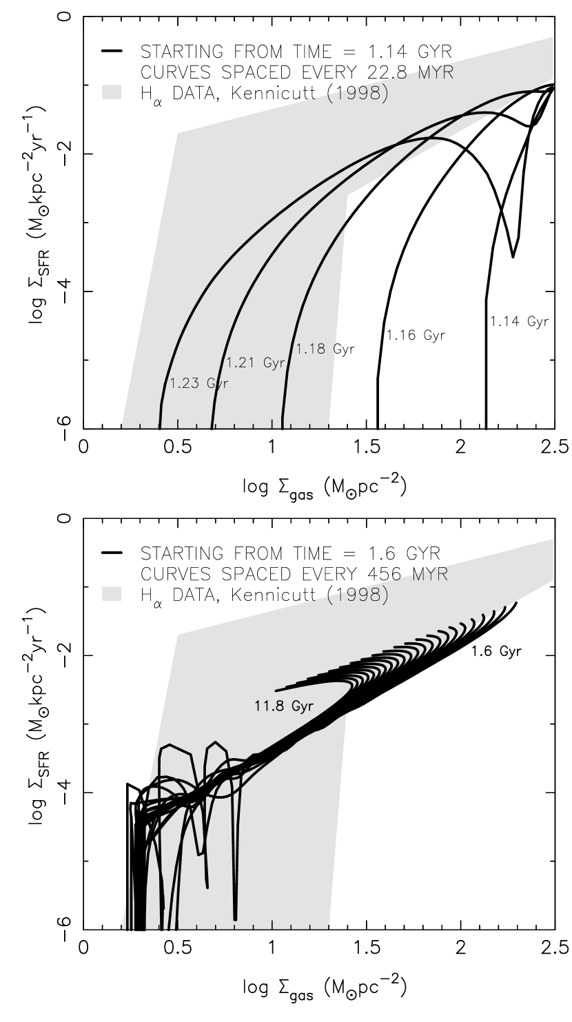
Figure 11: Time evolution of the star formation rate surface density as a function of the gas surface density in one of our simulations defined by $\Sigma_{g}^{i}=\Sigma_{0}/(1+(\frac{r}{r_{p}})^{4})$, with $r_{p}=5.12$ kpc, $r_{0}=2.56$ kpc, and $v_{0}=220$ km/s. Solid lines are our star formation rate profiles at times indicated on the figure. Shaded region is observational data by Kennicutt (1998).

Another test of the viscous model for star formation in galactic disks, is the comparison of the star formation rate with the gas surface density as a function of time.

On figure 11, we plot the results from our model with an initial gas profile given by $\Sigma_{g}^{i}=\Sigma_{0}/(1+(\frac{r}{r_{p}})^{4})$, with $r_{p}=5.12$ kpc, and evolving in a potential characterized by $r_{0}=2.56$ kpc and $v_{0}=220$ km/s (other results for this profile were shown in fig. 10). On the same plot we also indicate the observational constraints set by Kennicutt’s H$\alpha$ data (Kennicutt 1998) for the SFR surface density $\Sigma_{\rm SFR}$ and CO data for the gas surface density, $\Sigma_{gas}$. Top panel of fig. 11 gives results of the early evolution (up to 1.2 Gyr), whereas bottom panel of the same figure shows the late evolution (from 1.6 to 12 Gyr). There are two important remarks to make concerning this figure: the first is that one can clearly see star formation happening inside out, with the central region having the highest star formation rate in the beginning. The latter progressively decreases due to the lack of gas to fuel it at late times. But this monotonic behaviour only takes place after the radial velocity profile has settled down to the steady state solution, because we see in the top panel of fig. 11 that there are some regions with a high density of gas that form a low amount of stars in the early stage. This is due to outflows of gas for which we quench star formation. We explicitly only allow stars to form where the radial velocity is directed towards the center of the disk. The second point is that although we naturally reproduce the slope of the relationship and the cut-off at low gas surface densities seen in the data, the locus occupied by our curves at late stages is offset towards low values. This, however, should not be considered as a failure of the model, as the normalisation of the total gas mass is somewhat arbitrary. Had we started the simulation with 15 % of baryons in our dark matter potential instead of 5 % (which is also a reasonable cosmological value for the baryon fraction), the star formation rates and gas surface densities would have increased by a factor of three, bringing the model in perfect agreement with the observational data. Also, the picture would be more complicated if we introduced even a moderate amount of infall, because both star formation rate and gas surface density would also go up. Furthermore, as discussed at the end of section 5.4, had we taken a higher value for the viscosity, we would have found faster star formation timescales which would also have increased the star formation rates.

5.6 Angular momentum

Finally, for the rotating viscous disk, one might worry that, as pointed out by Lynden-Bell and Pringle (1974), the equilibrium is reached when a portion of fluid with negligible mass carries all the angular momentum to infinity while the rest of the gas collapses to the center. This would only exacerbate the angular momentum problem seen in N-Body + SPH simulations, if it were not for the fact that star formation has to proceed on a viscous timescale in order for galaxies to end up with exponential light profiles, so the redistribution of angular momentum cannot be very efficient. Although in the simulations presented in this paper, we do not take into account feedback via supernovae explosions or stellar winds that would reheat and redistribute the gas, we show that viscous evolution does not lead to a dramatic decrease in the specific angular momentum of the gas.

Figure 12: Comparison of the cumulative specific angular momentum profiles for the initial gas distribution (solid line) and both the final stellar (asterices) and gas (open circles) distributions, i.e. after 12 Gyr of viscous evolution. The dashed line shows the initial gas profiles. The exact analytic shapes of these profiles are given in tables 1 and  2. The core radius, $r_{0}$, of the gravitational potential is written in the lower right corner of each panel and $v_{0}$, the asymptotic circular velocity is 220 km/s in all simulations.

On figure 12 we plot the time evolution of the cumulative specific angular momentum, $j_{c}=J/M$, of both gas and stars. This quantity is obtained by computing the total amount of angular momentum in concentric gaseous/stellar disks and dividing it by the gaseous/stellar mass in these disks. There are a couple of things that we would like to emphasize on this figure. First is that in all the runs, the stellar angular momentum distribution closely follows the initial gas angular momentum distribution, which already points out that viscous redistribution of angular momentum must be small. This is particularly noticeable in the inner regions of the disk. Second, one can immediately see from figure 12 that the final gas angular momentum distribution is always higher than the initial one, especially at large radii. In fact, there is a clear trend that the steeper the initial gas density profile and rotation curve, the larger the discrepancy between the initial and final specific angular momenta of the gas. The reason for this is the following: since initial gas density profiles are generally decreasing functions of radius, equation 11 combined with equation 9 imply that the star formation rate is much higher in the center of disk galaxies. Hence star formation will proceed inside out, consuming gas with low specific angular momentum first. As a result, after 12 Gyr, the leftover gas is naturally located in the outer regions of the disk where the specific angular momentum is higher in general, and the viscous timescale so large that redistribution is minimal, naturally yielding an increase in the cumulative specific angular momentum.

6 Conclusions

We have performed the first numerical hydrodynamical simulations probing the viscous evolution of isothermal and non self-gravitating disk galaxies embedded in static dark halo potentials.

Despite the simplicity of such a model, where we have also neglected the return fraction of gas through stellar evolution, infall, and feedback, we obtain disks with approximately exponential stellar profiles, regardless of their initial gas profile and rotation curve as long as $t_{\star}\sim t_{visc}$. Moreover, we obtain fractions of gas and stars after $\sim$ 12 Gyr of viscous evolution that are consistent with observations, without having to invoke an efficiency parameter for star formation. Although a detailed explanation for the connection between the viscous timescale and star formation is yet to be worked out in details, this strongly suggests that the viscous timescale might indeed be the natural timescale for star formation. It is also a more appealing alternative than fine-tuning the initial conditions of proto-galactic clouds destined to form disks in order to obtain exponential stellar density profiles.

The specific results of our investigation are:

• When $t_{\star}\sim t_{visc}$, the resulting stellar profile is approximately exponential. When $t_{\star}$ is 10 times smaller than the viscous timescale then the initial gas profile is frozen into the stellar distribution and when $t_{\star}$ is 10 times larger than the viscous timescale then the stellar distribution is better described by a power law.

• Exponentials fit reasonably well the stellar profiles after $\sim$ 12 Gyr, regardless of the initial gas profile or the rotation curve. Furthermore, there is no requirement on conservation of specific angular momentum throughout star formation.

• For rotation curve profiles similar to Milky Way profiles, ($r_{0}=2.56$ kpc and $v_{0}=220$ km/s in $\Phi$), after $\sim$ 12 Gyr the stellar densities in the solar neighborhood and the final gas fraction in the disk are consistent with observations, provided the initial gas density profile is quite steep. This suggests that the viscous timescale gives the star formation efficiency naturally.

• The disk scale length, $r_{s}$, depends most strongly on the degree of central concentration of the initial gas density profile (figure 9). The steepness of the dark halo rotation curve introduces very little spread in the initial gas half mass radius, $r_{H}$, versus $r_{s}$ relation.

• The cumulative specific angular momentum of the final distribution of gas is always higher than the initial cumulative specific angular momentum of the gas due to inside out formation. The steeper the initial gas profile, the more important is the discrepancy between the cumulative specific angular momentum of the gas after $\sim$ 12 Gyr and its initial cumulative specific angular momentum. The cumulative specific angular momentum of the stars after $\sim$ 12 Gyr, on the other hand, closely matches the initial cumulative specific angular momentum of the gas.

• The slope of the star formation rate density versus gas surface density in the viscous disk models is in fair agreement with the observed one, and the cut-off seen at low gas surface densities in the observations is naturally reproduced.

Clearly, this work is a necessary first step which proves the ability of the BGK scheme to follow the physical processes occuring in a galactic disk. In following works, we shall focus on implementing more realistic conditions for the starting point of the simulation and the mechanisms driving the disk evolution. We also plan to extend the code to 3D and include self-gravity of both dark halo and gas.

Acknowledgements.  We are pleased to thank Kun Xu for providing us with a version of the BGK scheme employing a reconstruction of g from two half-Maxwellians. We also thank Stéphane Colombi for parallelizing the scheme. AS thanks Kevin Prendergast for invaluable discussions and Oxford University for its hospitality during the course of much of this work.

Appendix A Initial conditions

Here we give analytic expressions for the initial radial velocities, $v_{R}^{i}$, which correspond to the initial density profiles, $\Sigma_{g}^{i}$ we use in the paper, i.e. knowing $v_{C}$ from equation 8, we compute $v_{R}^{i}$ by solving the second Navier-Stokes equation (eq. 6). This yields:

• if $\Sigma_{g}^{i}(r)=\Sigma_{0}$ = constant,

  $$v_{R}^{i}(r)=-\nu\frac{r(r^{2}+4r_{0}^{2})}{(r_{0}^{2}+r^{2})(2r_{0}^{2}+r^{2})}\\$$ (12)

• if $\Sigma_{g}^{i}(r)=\Sigma_{0}/[1+(\frac{r}{r_{p}})^{2}]$

  $$v_{R}^{i}(r)=-\nu\frac{r(4r_{p}^{2}r_{0}^{2}+r^{2}r_{p}^{2}+2r^{2}r_{0}^{2}-r^{4})}{(r_{0}^{2}+r^{2})(2r_{0}^{2}+r^{2})(r_{p}^{2}+r^{2})}\\$$ (13)

• if $\Sigma_{g}^{i}(r)=\Sigma_{0}/[1+(\frac{r}{r_{p}})^{4}]$

  $$v_{R}^{i}(r)=-\nu\frac{r(4r_{p}^{4}r_{0}^{2}+r^{2}r_{p}^{4}-3r^{6})}{(r_{0}^{2}+r^{2})(2r_{0}^{2}+r^{2})(r_{p}^{4}+r^{4})}\\$$ (14)

• if $\Sigma_{g}^{i}(r)=\Sigma_{0}\exp(-r/r_{s})$

  $$v_{R}^{i}(r)=-\nu\frac{r(4r_{s}r_{0}^{2}+r^{2}r_{s}^{2}-rr_{0}^{2}-r^{3})}{(r_{0}^{2}+r^{2})(2r_{0}^{2}+r^{2})r_{s}}\\$$ (15)

Note that these initial conditions for the radial velocity have quite different asymptotic properties. For instance, the initial radial velocity corresponding to the constant density profile (eq 12) is always negative, meaning the gas is constantly flowing in as the steady state radial velocity is also always negative (eq 9). However, both radial velocities go to zero like $r^{-1}$ at large radii for the initial power profiles (eq 13 and 14), which means that there should be a small initial outflow of gas in these simulations. Finally the initial radial velocity profile corresponding to an initial exponential density profile (eq 15) can have arbitrarily high outflows at large radii, depending on the value of $r_{s}$: the smaller the value, the more important the outflow since $v_{R}^{i}\propto r_{s}^{-1}$.

References

- [] Barnes J. E. & Efstathiou G., 1987, ApJ, 319, 575
- [] Bhatnagar P.L., Gross E.P., Krook M., 1954, Phys. Rev., 94, 511
- [] Binney J. & Tremaine S., 1987, Galactic Dynamics, Princeton University Press
- [] Chromey F. R., 1978, AJ, 83, 162
- [] Clarke C. J., 1989, MNRAS, 238, 283
- [] Cole S., Aragon-Salamanca A., Frenk C. S., Navarro J. F. & Zepf S. E., 1994, MNRAS, 271, 781
- [] Contardo G., Steinmetz M. & Fritz-von Alvensleben U., 1998, ApJ, 507, 497
- [] Crampin D. J. & Hoyle F., 1964, ApJ, 140, 99
- [] Dalcanton J. J., Spergel D.N., Summers F. J., 1997, ApJ, 482, 659
- [] Duschl W. J., Strittmatter P. A. & Biermann P. L, 2000, A&A, 357, 1123
- [] Ferguson A. & Clarke C. J., 2001, MNRAS, in press, astro-ph/0103205
- [] Fich M. & Blitz L., 1984, ApJ, 279, 125
- [] Firmani C., Hernandez X. & Gallagher J., 1996, A&A, 308, 403
- [] Gerritsen J. P. E. & Icke V., 1997, A&A, 325, 972
- [] Gunn J. E. , 1982, in Astrophysical Cosmology, ed. H. A. Brück, G. V. Coyne, and M. S. Longair (Vatican: Pontificia Academia Scientiarum), 248
- [] Hernquist L., 1990, ApJ, 356, 359
- [] Huynh H. T., 1995, SIAM J. Numer. Anal., 32, 1565
- [] Kauffmann G. A. M., White S. D. M. & Guiderdoni B., 1993, MNRAS, 264, 201
- [] Katz N., 1992, ApJ, 391, 502
- [] Katz N. & Gunn J. E., 1991, ApJ, 377, 365
- [] Kennicutt R. C., 1998, ARA&A, 36, 189
- [] Kim C. & Jameson A., 1998, J. Comput. Phys., in press
- [] Kuijken K. & Gilmore G., 1989, MNRAS, 239, 605
- [] Lacey C. G. & Fall, M., 1985, ApJ, 290, 154
- [] Lin D. C. N. & Pringle J. E., 1987, ApJ, 320, L87
- [] Lynden-Bell D. & Pringle J. E., 1974, MNRAS, 168, 603
- [] Mestel L., 1963, MNRAS, 126, 553
- [] Mihos J. C. & Hernquist L., 1994, ApJ, 437, 611
- [] Mo H., Mao S. & White S. D. M., 1998, MNRAS, 295, 319
- [] Navarro J. F., Frenk C. S. & White S. D. M., 1996, ApJ, 462, 563
- [] Navarro J. F. & Steinmetz M., 1997, ApJ, 478, 13
- [] Olivier S., Blumenthal G. R., Primack J.R., 1991, MNRAS, 252, 102
- [] Prantzos N. & Aubert O., 1995, A&A, 302, 69
- [] Prendergast K. H., Xu K., 1993, J. Comput. Phys., 109, 53
- [] Press W. H. & Schechter P., 1974, ApJ, 187, 425
- [] Richard d. & Zahn J.-P., 1999, A&A, 347, 734
- [] Saio H. & Yoshii Y., 1990, ApJ, 363, 40
- [] Sanders R. H. & Prendergast K. H., 1974, ApJ, 188,489
- [] Silk J. & Norman C., 1981, ApJ, 247, 59
- [] Silk J., 2001, MNRAS, in press, astro-ph/0010624
- [] Slyz A. & Prendergast K. H., 1999, Astron. Astrophys. Suppl. Ser., 139, 199
- [] Sommer-Larsen J., Gelato S. & Vedel H., 1999, ApJ, 519, 501
- [] Somerville R. S. & Primack J. R., 1999, MNRAS, 310, 1087
- [] Springel V., 1999, MNRAS, 312. 859
- [] Steinmetz M. & Müller E., 1995, MNRAS, 276, 549
- [] van der Kruit P.C., 1987, A&A, 173, 59
- [] Vedel H., Hellsten U. & Sommer-Larsen J., 1994, MNRAS, 271, 743
- [] Warren M. S., Quinn P. J., Salmon J. K. & Zurek W. H., 1992, ApJ, 399, 405
- [] Weil M. L., Eke V. R. & Efstathiou G., 1998, MNRAS, 300, 773
- [] Xu K., 1998, Gas-Kinetic Schemes for Unsteady Compressible Flow Simulations, VKI report 1998-03 von Karmann Institute Lecture Series
- [] Xu K. & Prendergast K. H., 1994, J. Comput. Phys., 114, 9
- [] Yoshii Y. & Sommer-Larsen J., 1989, MNRAS, 236, 779