Derivation of the Mass Distribution of Extrasolar Planets with MAXLIMA - a Maximum Likelihood Algorithm

Abstract

We construct a maximum-likelihood algorithm - MAXLIMA, to derive the mass distribution of the extrasolar planets when only the minimum masses are observed. The algorithm derives the distribution by solving a numerically stable set of equations, and does not need any iteration or smoothing. Based on 50 minimum masses, MAXLIMA yields a distribution which is approximately flat in $\log M$, and might rise slightly towards lower masses. The frequency drops off very sharply when going to masses higher than 10 $M_{J}$, although we suspect there is still a higher mass tail that extends up to probably 20 $M_{J}$. We estimate that 5% of the G stars in the solar neighborhood have planets in the range of 1–10 $M_{J}$ with periods shorter than 1500 days. For comparison we present the mass distribution of stellar companions in the range of 100–1000$M_{J}$, which is also approximately flat in $\log M$. The two populations are separated by the “brown-dwarf desert”, a fact that strongly supports the idea that these are two distinct populations. Accepting this definite separation, we point out the conundrum concerning the similarities between the period, eccentricity and even mass distribution of the two populations.

1 INTRODUCTION

Since the detection of the first few extrasolar planets their mass distribution was recognized to be a key feature of the growing new population. In particular, the potential of the high end of the mass distribution to separate between planets on one side and brown dwarfs and stellar companions on the other side was pointed out by numerous studies (e.g., Basri & Marcy 1997; Mayor, Queloz & Udry 1998; Mazeh, Goldberg & Latham 1998). A clear mass separation between the two populations could even help to clarify one of the very basic questions concerning the population of extrasolar planets — the precise definition of a planet (Burrows et al. 1997; see a detailed discussion by Mazeh & Zucker 2001). The lower end of the mass distribution could indicate how many Saturn- and Neptune-like planets we expect on the basis of the present discoveries, a still unsurveyed region of the parameter space of extrasolar planets.

The present number of known extrasolar planets — more than 60 are known (Encyclopedia of extrasolar planets, Schneider 2001), offers an opportunity to derive a better estimate of the mass distribution of this population. In order to use the derived masses of the extrasolar planets we have to correct for two effects. The first one is the unknown orbital inclination, which renders the derived masses only minimum masses. The second effect is due to the fact that stars with too small radial-velocity amplitudes could not have been detected as radial-velocity variables. Therefore, planets with masses too small, orbital periods too large, or inclination angles too small are not detected.

The effect of the unknown inclination of spectroscopic binaries was studied by numerous papers (e.g., Mazeh & Goldberg 1992; Heacox 1995; Goldberg 2000), assuming random orientation in space. Heacox (1995) calculates first the minimum mass distribution and then uses its relation to the mass distribution to derive the latter. This calculation amplifies the noise in the observed data, and necessitates the use of smoothing to the observed data. Mazeh & Goldberg (1992) introduce an iterative algorithm whose solution depends on the initial guess. In the present work we followed Tokovinin (1991, 1992) and constructed an algorithm — MAXimum LIkelihood MAss, to derive the mass distribution of the extrasolar planets with a maximum likelihood approach. MAXLIMA assumes that the planes of motion of the planets are randomly oriented in space and derives the mass distribution directly by solving a set of numerically stable linear equations. It does not require any smoothing of the data nor any iterative algorithm. MAXLIMA also offers a natural way to correct for the undetected planets.

The randomness of the orbital planes of the discovered planets were questioned recently by Han et al. (2001), based on the analysis of Hipparcos data. However a few very recent studies (Pourbaix 2001; Pourbaix & Arenou 2001; Zucker & Mazeh 2001a,b) showed that the Hipparocos data do not prove the nonrandomness of the orbital planes, allowing us to apply MAXLIMA to the sample of known minimum masses of the planet candidates.

In the course of preparing this paper for publication we have learned about a similar paper by Jorissen, Mayor & Udry (2001) that was posted on the Astrophysics e-Print Archive (astro-ph). Like Heacox (1995), Jorrisen et al. derive first the distribution of the minimum masses and then apply two alternative algorithms to invert it to the distribution of planet masses. One algorithm is a formal solution of an Abel integral equation and the other is the Richardson-Lucy algorithm (e.g., Heacox 1995). The first algorithm necessitates some degree of data smoothing and the second one requires a series of iterations. The results of the first algorithm depend on the degree of smoothing applied, and those of the second one on the number of iterations performed. MAXLIMA has no built-in free parameter, except the widths of the histogram bins. In addition, Jorissen et al. did not apply any correction to the selection effect we consider here, and displayed their results on a linear mass scale. We feel that a logarithmic scale can illuminate some other aspects of the distribution. Despite all the differences, our results are completely consistent with those of Jorrisen et al., the sharp cutoff in the planet mass distribution at about 10 $M_{J}$, and the small high-mass tail that extends up to about 20 $M_{J}$ in particular.

Section 2 presents MAXLIMA, while section 3 presents our results. Section 4 discusses briefly our findings.

2 MAXLIMA

2.1 The Unknown Inclination

Our goal is to estimate the probability density function (PDF) of the secondary mass — $f_{m}(m)dm$, given a set of observed minimum masses {$y_{j};j=1,N\}$, where $y_{j}=m_{j}\times\sin i_{j}$, $m_{j}$ is the mass of the j-th planet and $i_{j}$ is its inclination. Within certain assumptions and limitations, MAXLIMA finds the function $f_{m}$ that maximizes the likelihood of observing these minimum masses.

Note that the present realization of MAXLIMA uses the approximation that the mass of the unseen companion is much smaller than the primary mass. Within this approximation $y_{j}$ can be derived from the observations of each system, given the primary mass. In general, when the secondary mass is not so small, the value of $m_{j}\times\sin i_{j}$ cannot be derived from the observations, and a more complicated expression has to be used. Nevertheless, the extension of MAXLIMA to those cases is straightforward, and will be worked out in details in a separate paper.

We assume that the directions of the angular momenta of the systems are distributed isotropically, which will cause $\sin i$ to have a PDF of the form:

$$f_{s}(s)\,ds=\frac{s}{\sqrt{1-s^{2}}}\,ds\ ,$$

where we denote $\sin i$ by $s$. We further assume that the planet mass and its orbital inclination are uncorrelated, and therefore the joint PDF of $\sin i$ and the planet mass have the form:

$$f_{ms}(m,s)\,dm\,ds=f_{m}(m)\ \frac{s}{\sqrt{1-s^{2}}}\,dm\,ds\ .$$

Now, define a variable $y=m\times\sin i=m\times s$, which has the PDF

$$f_{y}(y)dy=\int{f_{m}(m){f_{s}(y/m)\over m}}\,dm\,dy=\int{{f_{m}(m)\over m}{(y/m)\over\sqrt{1-(y/m)^{2}}}}\,dm\,dy\ .$$

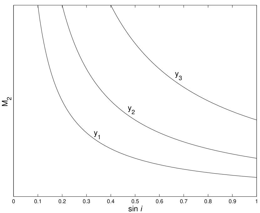
Figure 1: Three contours of constant $y$’s in the $m-s$ plane.

A sketch of contours of constant $y$ in the $m-s$ parameter space is plotted in Figure 1.

We wish to estimate $f_{m}(m)$ in the form of a histogram with K bins, between the limits $m_{min}\leq m<m_{max}$. We thus consider a partition of the interval $[m_{min},m_{max})$:

$$m_{min}=m_{1},m_{2},\ldots,m_{K+1}=m_{max}\ ,$$

for which the PDF gets the form:

$$f_{m}(m)\equiv b_{k},\;{\rm if\ }m_{k}\leq m<m_{k+1},\;{\rm for\ }k=1,\ldots,K.$$

Note, that the function $f_{m}(m)$ is supposed to be a probability density function, and therefore its integral must equal one:

$$\sum_{k=1}^{K}b_{k}\Delta m_{k}=1\ ,$$ (1)

where $\Delta m_{k}\equiv m_{k+1}-m_{k}$ for $k=1,\ldots,K$.

The PDF of $y$ then gets the form:

$$f_{y}(y)\,dy = \sum_{k=1}^{K}\int_{m_{k}}^{m_{k+1}}\frac{b_{k}}{m}\frac{y/m}{\sqrt{1-(y/m)^{2}}}\,dm\,dy$$

$$= \sum_{k=1}^{K}b_{k}\int_{m_{k}}^{m_{k+1}}\frac{1}{m}\frac{y/m}{\sqrt{1-(y/m)^{2}}}\,dm\,dy\ ,$$

where the integrals do not depend on $f_{m}(m)$ at all, but only on the intervals borders and $y$.

Now we can solve our problem in a maximum-likelihood fashion by finding the set of $b_{k}$’s that maximizes the likelihood of the actually observed values - ${y_{j}}$. The likelihood function is:

$$\mathcal{L}(b_{1},\ldots,b_{K};y_{1},\ldots,y_{N}) = \prod_{j=1}^{N}f_{y}(y_{j})$$

$$= \prod_{j=1}^{N}\sum_{k=1}^{K}b_{k}\int_{m_{k}}^{m_{k+1}}\frac{1}{m}\frac{y_{j}/m}{\sqrt{1-(y_{j}/m)^{2}}}\,dm$$

$$= \prod_{j=1}^{N}\sum_{k=1}^{K}A_{jk}b_{k}\ ,$$

where

$$A_{jk}=\cases{0&$m_{k+1}\leq y_{j}$\cr\int_{y_{j}}^{m_{k+1}}\frac{1}{m}\frac{y_{j}/m}{\sqrt{1-(y_{j}/m)^{2}}}\,dm&$m_{k}\leq y_{j}<m_{k+1}$\cr\int_{m_{k}}^{m_{k+1}}\frac{1}{m}\frac{y_{j}/m}{\sqrt{1-(y_{j}/m)^{2}}}\,dm&$y_{j}<m_{k}$ \ ,\cr}$$ (2)

and the integrals are easily calculated even analytically.

In the appendix we present an elegant way to find the $b_{k}$’s that maximize $\log\mathcal{L}$ directly, without any iterations.

2.2 Simulation

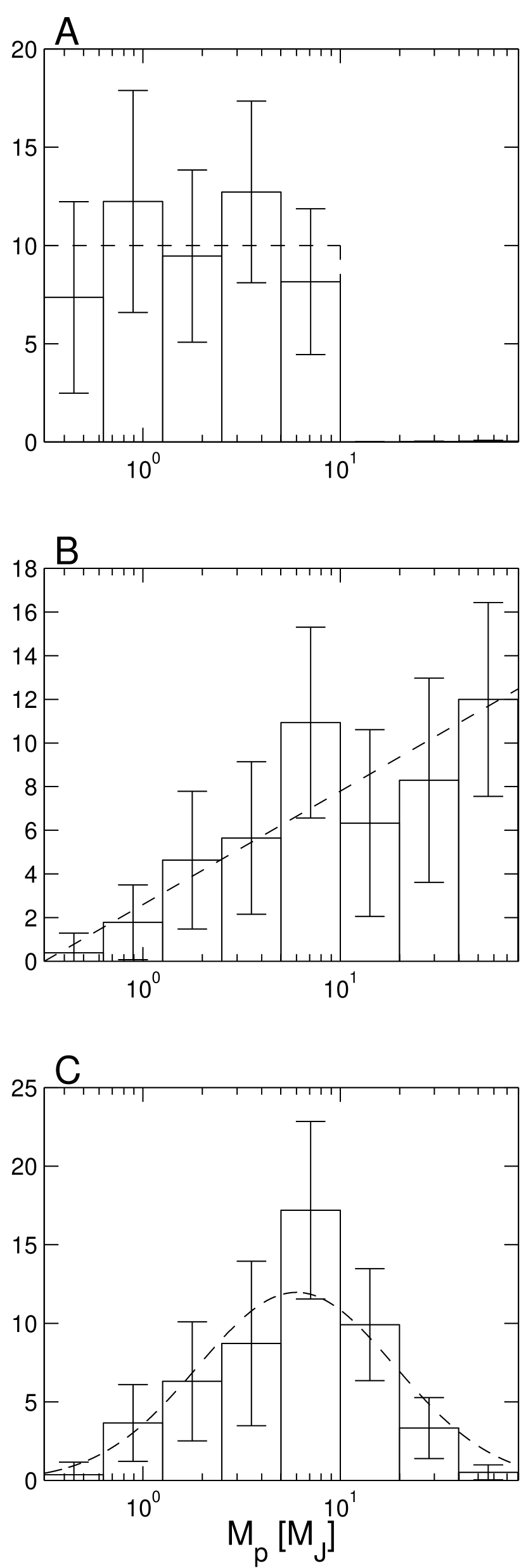
Figure 2: Three simulations of MAXLIMA. In all three panels the dashed line shows the input distribution and the histogram the results of MAXLIMA.

In order to check the performance of MAXLIMA and its realization we have performed several simulations, some of which are presented in Figure 2. In those simulations we generated an artificial sample of planets drawn from populations with different PDFs of the planet masses, and inclinations oriented isotropically in space. To make the simulation similar to the present work we chose the size of each sample to be 50 planets. We assumed no selection effects. We then applied MAXLIMA to the simulated sample, the results of which are plotted in Figure 2.

The three examples of Figure 2 clearly show the power of MAXLIMA.

2.3 Selection Effect: Undetected Planets

We assume that the sample is constructed of planets with period, $P$, between $P_{\rm min}\leq P\leq P_{\rm max}$. We further assume that the search for planets discovered all radial-velocity variables with amplitude $K$ larger than $K_{\rm min}$. We have to correct for planets not detected because they induce $K$ smaller than the threshold. To do that we note that the amplitude can be written as

$$K(P,M_{p},M_{1},\sin i)=204\,\left({P\over{{\rm day}}}\right)^{-1/3}\,\left({M_{1}\over{M_{\odot}}}\right)^{-2/3}\,\left({M_{p}\over{M_{Jup}}}\right)\,\sin i\ \,\ \rm m\,s^{-1}\ .$$ (3)

The expression $M_{p}\times\sin i$ is actually our $y$. For any given value of $y$ and $M_{1}$ we can derive the maximum possibly detected period — $P_{\rm max-detect}$, given $K_{\rm min}$. This implies that if we know the period distribution and we assume that the period is uncorrelated to the mass distribution, we can estimate for each of the given $y$’s the fraction of planets with long periods that were not detected with the same $y$. This means that to correct for the undetected planets with long periods we have to consider each of the j-th detected systems as representing some $\alpha_{j}$ planets. If $P_{\rm max-detect}$ is smaller than $P_{\rm max}$, then $\alpha_{j}$ is larger than unity. Otherwise $\alpha_{j}$ is equal to unity.

We then can write a new generalized likelihood as:

$$\mathcal{L}(b_{1},\ldots,b_{K};y_{1},\ldots,y_{N};\alpha_{1},\ldots,\alpha_{N}) = \prod_{j=1}^{N}\left(f_{y}(y_{j})\right)^{\alpha_{j}}$$

$$= \prod_{j=1}^{N}\left(\sum_{k=1}^{K}b_{k}\int_{m_{k}}^{m_{k+1}}\frac{1}{m}\frac{y_{j}/m}{\sqrt{1-(y_{j}/m)^{2}}}\,dm\right)^{\alpha_{j}}$$

$$= \prod_{j=1}^{N}\left(\sum_{k=1}^{K}A_{jk}b_{k}\right)^{\alpha_{j}}\ .$$

The Appendix shows an easy way used by MAXLIMA to find a maximum to $\log\mathcal{L}$.

For simplicity we consider only circular orbits. Eccentricity introduces two effects (Mazeh, Latham & Stefanik 1996), the first of which is the dependence of $K$ on the eccentricity $e$. Equation (3) should include an additional factor of $(1-e^{2})^{-1/2}$, which causes $K$ to increase for increasing $e$. The other factor is the dependence of the detection threshold $K_{\rm min}$ on $e$. Our simplifying assumption about the constancy of $K_{\rm min}$ throughout the sample breaks down when we consider eccentric orbits. This is so because for eccentric orbits the velocity variation tends to concentrate around the periastron passage, and therefore $K_{\rm min}$ increases for increasing eccentricity. These two effects tend to cancel each other (Fischer & Marcy 1992), the net effect depends on the characteristics of the observational search. By running numerical simulations Mazeh et al. (1996) have found that if the detection limit depends on the r.m.s. scatter of the observed radial-velocity measurements, the two effects cancel each other for any reasonable eccentricity. We therefore chose not to include the eccentricity of the planets in our analysis.

3 ANALYSIS AND RESULTS

To apply MAXLIMA to the current known sample of extrasolar planets we considered all known planets and brown dwarfs as of April 2001. We consider only G- or K-star primaries and therefore excluded Gls 876 from the sample.

Obviously, the present sample in not complete. In particular, not all planets with long periods and small induced radial-velocity amplitudes were discovered and/or announced. To acquire some degree of completeness to our sample we have decided, somewhat arbitrarily, to exclude planets with periods longer than 1500 days and with radial-velocity amplitudes smaller than 40 m/s. The values of these two parameters determine the correction of MAXLIMA for the selection effect, for which we assumed a period distribution which is flat in $\log P$. This choice of parameters also implies that our analysis applies only to planets with periods shorter than 1500 days. We further assumed that the primary mass is 1 $M_{\odot}$ for all systems.

In order to be consistent with the selection effects and the correction we applied, we included in our analysis only planets that were discovered by the high precision radial-velocity searches. We had to exclude HD 114762 and similar objects that were discovered by other searches (e.g., Latham et al. 1989; Mayor et al. 1992; Mazeh et al. 1996). This does not mean that we assume anything about their nature in this stage of the study. Table 1 lists all the known planets with G star primaries from the high precision radial-velocity studies. Planets excluded from our analysis are marked by an asterisk. We did not take into account the known inclination of the planet around HD 209458. All together we are left with 50 planets.

The results of MAXLIMA are presented in the lower panel of Figure 3 on a logarithmic mass scale. Each bin is 0.3 dex wide, which means about a factor 2 in mass. The value of each bin is the estimated number of planets found in the corresponding range of masses in the known sample of planets, after correcting for the undetected systems. To estimate the uncertainty of each bin we ran 5000 Monte Carlo simulations and found the r.m.s. of the derived values of each bin. Therefore, the errors plotted in the figure represent only the statistical noise of the sample. Obviously, any deviation from the assumptions of our model for the selection effect induces further errors into the histogram, the assumed period distribution in particular. This is specially true for the first bin, where the actual number of systems is small and the correction factor large. The value of the first bin is sensitive, for example, to the assumed $K_{\rm min}$. Assuming $K_{\rm min}$ of 50 m/s increased the value of the first bin by more than 50%.

To compare the mass distribution of the planets with that of the stellar secondaries we plot the latter on the same scale in an adjacent panel of Figure 3. We plot here only two bins, with masses between 100 and 1000 $M_{J}$. We follow the work of Mazeh (1999b) and Mazeh and Zucker (2001), and used for those bins subsamples of binaries found by the CfA radial-velocity search for spectroscopic binaries (Latham 1985) in the Carney & Latham (1987) sample of the high-proper-motion stars (Latham et al. 2000; Goldberg et al. 2000). For the smaller bin we used a subsample that included only the Galaxy disk stars (Goldberg 2000), and for the larger-mass bin a subsample of this sample that included only primaries with masses higher than 0.7 $M_{\odot}$. The values of those two bins were derived with the algorithm of Mazeh & Goldberg (1992).

Note that the upper panel does not have any estimate of the values of the bins with masses smaller than 100 $M_{J}$. This is so because the CfA search does not have the sensitivity to detect secondaries in that range. On the other hand, the lower panel does include information on the bins below 100 $M_{J}$. This panel presents the results of the high-precision radial-velocity searches, and these searches could easily detect stars with secondaries in the range of, say, 20–100 $M_{J}$. We assume that these binaries were not excluded from the various radial-velocity searches at the first place, and further assume that all, or at least most, findings of the various research groups corresponding to this range of masses were already published. If these two assumptions are correct, then the lower panel does represent the frequency of secondaries in the mass range of 20–100 $M_{J}$. This panel shows that the frequency of secondaries in this range of masses is close to zero. The present analysis is not able to tell whether this “brown-dwarf desert” extends up to 60, 80 or 100 $M_{J}$.

The relative scaling of the planets and the stellar companions is not well known. The spectroscopic binaries come from well defined samples – 577 stars for the lower-mass bin, and 312 stars for the higher-mass stars (Goldberg 2000). However, this is not the case for the detected planets, specially because the sample of published planets is not complete and also because the search samples of the different groups are not well documented in the public domain. We assumed, somewhat arbitrarily, that they come from a sample of 1000 stars, and scaled the stellar bins accordingly. We also rescaled the stellar bins to account for the fact that their bins are larger, and their period range extends up to 3000 days, assuming a flat distribution in $\log P$. Therefore the values of the stellar bins are our best estimate for the number of binaries for 1000 stars within a mass range of 0.3 dex, and up to a period of 1500 days.

Obviously the relative scaling of the two panels has a large uncertainty. This scaling uncertainty is not reflected in the error bars of the higher panel. Nevertheless we think that the comparison is illuminating, as will be discussed in the next section.

4 DISCUSSION

The grand picture that is emerging from Figure 3 strongly indicates that we have here two distinct populations. The two populations are separated by a “gap” of about one decade of masses, in the range between 10 and 100 $M_{J}$. Such a gap was already noticed by many early studies (Basri & Marcy 1997; Mayor, Queloz & Udry 1998; Mayor, Udry & Queloz 1998; Marcy & Butler 1998). Those early papers binned the mass distribution linearly. Here we follow our previous work (Mazeh et al. 1998) and use a logarithmic scale to study the mass distribution, because of the large range of masses, 0.5–1000 $M_{J}$, involved. The logarithmic scale has also been used by Tokovinin (1992) to study the secondary mass distribution in spectroscopic binaries, and was suggested by Black (1998) to study the mass distribution of the planetary-mass companions (see also Mazeh 1999a,b; Mazeh & Zucker 2001; Mayor et al. 2001). The gap or the “brown-dwarf desert” are consistent also with the finding of Halbwachs et al. (2000), who used Hipparcos data and found that many of the known brown-dwarf candidates are actually stellar companions.

We will assume that the two populations are the planets, at the low-mass side of Figure 3, and the stellar companions at the high-mass end of the figure. Interestingly, the mass distribution of single stars extends far below 100 $M_{J}$ (e.g., Zapatero Osorio et al. 2000; Lucas & Roche 2000), indicating that the gap separating the two populations of companions apparently does not exist in the population of single stars/brown dwarfs. This difference probably indicates different formation processes for single and secondary objects.

The distribution we derived in Figure 3 suggests that the planet mass distribution is almost flat in $\log M$ over five bins — from 0.3 to 10 $M_{J}$. Actually, the figure suggests a slight rise of the distribution towards smaller masses. The distinction between these two distributions is not possible at this point, when our knowledge about planets with sub-Jupiter masses is very limited. At the high-mass end of the planet distribution the mass distribution dramatically drops off at 10 $M_{J}$, with a small high-end tail in the next bin. Although the results are still consistent with zero, we feel that the small value beyond 10 $M_{J}$ might be real. The dramatic drop at 10 $M_{J}$ and the small high-mass tail agree with the findings of Jorissen et al. (2001).

Examination of the two panels of Figure 3 suggests that per equal dex range of masses the frequency of stellar secondaries is higher than that of the planets by a factor of about 2. As we emphasized in the previous section, this is a very preliminary result that should be checked by future observations. Nevertheless, the frequency of planets is impressive by itself. Our results indicate that about 5% of the stars have planets with masses between 1 and 10 $M_{J}$. This is so because the number of multiple planets in this sample is small, so the number of planets considered in the figure is about the number of stars found to have one or more planets. If this frequency extends further down the mass axis to Earth masses, we might find that more than 10% of the stars have planets with periods shorter than 1500 days.

The analysis presented here raises the question what mechanism can produce flat or approximately flat mass distribution of planets up to 10 $M_{J}$. What determines the mass of the forming planet? The present paradigm assumes that planets were formed out of a protoplanetary disk. Is it the mass, density, angular momentum or the viscosity of the disk that determined the planet mass? If planets were formed by accreting gas onto a rocky core, is the planet mass determined also by the location or evolutionary phase of the formation of the rocky core? Any detailed model of planet formation should account for this mass distribution.

The clear distinction between the two populations suggests that planets and stellar companions were formed by two different processes. This is so despite the striking similarity between the distributions of the eccentricities and periods of the two populations (Heacox 1999; Stepinski & Black 2000, 2001; Mayor & Udry 2000; Mazeh & Zucker 2001). Even the mass distributions of the two populations might be very similar — approximately flat in $\log M$. This is still a conundrum that any formation model for planets as well as for binaries needs to solve.

Appendix

We want to find the maximum likelihood to observe a given set of observed minimum masses $\{y_{j};j=1,N\}$. As usual, it is easier to maximize the logarithm of the likelihood function:

$$\log\mathcal{L}=\sum_{j=1}^{N}\alpha_{j}\times\log\left(\sum_{k=1}^{K}A_{jk}b_{k}\right)\ ,$$

where each $A_{jk}$ depends on the corresponding $y_{j}$ through Equation (2).

The $b_{k}$’s are not all independent. They are constrained by Equation (1), and therefore we modify our target function by adding a Lagrange multiplier term:

$$\log\mathcal{L}=\sum_{j=1}^{N}\alpha_{j}\times\log\left(\sum_{k=1}^{K}A_{jk}b_{k}\right)+\lambda\left(\sum_{k=1}^{K}b_{k}\Delta m_{k}-1\right)\ .$$

The optimization is performed by equating the partial derivatives of this target function to zero:

$$\frac{\partial\log\mathcal{L}}{\partial b_{k}} = \sum_{j=1}^{N}\frac{\alpha_{j}\times A_{jk}}{\sum_{l=1}^{K}A_{jl}b_{l}}+\lambda\Delta m_{k}=0,\ {\rm for\ }k=1,\ldots,K$$

$$\frac{\partial\log\mathcal{L}}{\partial\lambda} = \sum_{k=1}^{K}b_{k}\Delta m_{k}-1=0\ .$$

The parameter $\lambda$ is eliminated quite easily. We first multiply each of the $K$ equations by the corresponding $b_{k}$ and then sum them up to get:

$$\sum_{k=1}^{K}\sum_{j=1}^{N}\frac{\alpha_{j}\times A_{jk}b_{k}}{\sum_{l=1}^{K}A_{jl}b_{l}}+\lambda\sum_{k=1}^{K}b_{k}\Delta m_{k}=0\ .$$

Changing the order of summation reduces the first term, after a simple manipulation, to simply

$$N_{eff}=\sum_{j=1}^{N}\alpha_{j}\ .$$

Using the constraint reduces the second term to $\lambda$, and we finally get:

$$N_{eff}+\lambda=0\ ,$$

and we can simply set $\lambda=-N_{eff}$. The $K$ equations we are now left with are:

$$\sum_{j=1}^{N}\alpha_{j}\times A_{jk}\frac{1}{\sum_{l=1}^{K}A_{jl}b_{l}}=N_{eff}\Delta m_{k}\ .$$

We have a set of $K$ non-linear equations in $K$ variables - $b_{k}$’s.

An elegant reduction of the complexity of the problem can be achieved if we set $K$ to $N$, by assigning $m_{k}\equiv y_{k}$ for $k=1,\ldots,N$. Let us also denote (remember that now $K=N$):

$$h_{j}\equiv\frac{1}{\sum_{l=1}^{N}A_{jl}b_{l}}$$ (1)

The $N$ equations now look like:

$$\sum_{j=1}^{N}\alpha_{j}\times A_{jk}h_{j}=N_{eff}\Delta m_{k}\ ,$$ (2)

which is a system of $N$ linear equations in the $N$ variables $h_{j}$. We can easily solve for them. The problem is even more easily solved when we note that the matrix $A_{jk}$ is upper-triangular and thus the amount of computations needed for the solution is smaller. Furthermore, examination of the integrals involved in the calculation of $A_{jk}$ (Eq. 2) shows that the matrix is very close to being diagonally-dominated, and therefore the set of linear equations is numerically stable. Having solved for $h_{j}$ we face again a similar system of linear equations in order to solve for $b_{k}$, coming from the definition of $h_{j}$:

$$\sum_{l=1}^{N}A_{jl}b_{l}=\frac{1}{h_{j}}.$$

In this system the matrix is the transposed matrix of the previous system of linear equations if the $\alpha_{j}$’s are all equal to unity.

Obviously, we wish to estimate the densities of our original intervals. But these are easily calculable from the $N$ densities $b_{k}$ calculated above, as simple linear combinations.

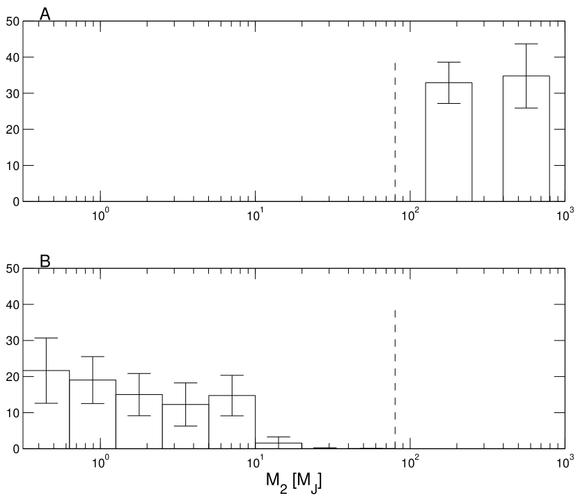
Figure 3: The mass distributions of the planets and the stellar companions

Table 1: Substellar companions list

Name	$M\sin i$	$P$	$K$
	($M_{J}$)	(days)	(m s-1)
∗HD 83443 b	0.16	29.83	14
∗HD 16141	0.215	75.82	11
∗HD 168746	0.24	6.41	28
∗HD 46375	0.249	3.02	35
HD 83443 c	0.34	2.985	56
∗HD 108147	0.34	10.88	37
HD 75289	0.42	3.51	54
51 Peg	0.47	4.23	56
BD -10°3166	0.48	3.487	61
∗HD 6434	0.48	22.09	37
HD 187123	0.48	3.10	69
∗Gliese 876 c	0.56	30.12	81
HD 209458	0.69	3.52	86
$\upsilon$ And b	0.69	4.617	71
HD 192263	0.787	24.36	68
HD 38529	0.81	14.32	54
HD 179949	0.84	3.09	101
55 Cnc	0.84	14.65	77
${}^{\ast}\epsilon$ Eri	0.86	2502.1	19
∗HD 82943 c	0.88	222	34
HD 121504	0.89	64.6	45
HD 130322	1.02	10.72	115
HD 37124	1.04	155.7	43
$\rho$ CrB	1.1	39.65	67
HD 52265	1.13	118.96	45
∗HD 177830	1.22	391.6	34
HD 217107	1.27	7.13	140
HD 210277	1.28	437	41
∗HD 27442	1.43	426.5	34
16 Cyg B	1.5	801	44
HD 74156 b	1.56	51.6	108
HD 134987	1.58	259.6	50
HD 82943 b	1.63	445	46
∗Gliese 876 b	1.89	61.02	210
HD 160691	1.97	743	54
HD 19994	2.0	454	45
HD 213240	3.7	759	91
$\upsilon$ And c	2.06	240.6	58
HD 8574	2.23	228.8	76
HR 810	2.26	320.1	67
47 UMa	2.39	1090	45
HD 12661	2.79	252.7	88
HD 169830	2.96	230.4	83
∗14 Her	3.3	1654	73
GJ 3021	3.32	133.82	164
HD 92788	3.34	326.7	100
HD 80606	3.41	111.8	414
HD 195019	3.47	18.2	272
$\tau$ Boo	3.87	3.31	469
Gliese 86	4	15.78	380
$\upsilon$ And d	4.10	1313	68
HD 50554	4.9	1279	95
HD 190228	5	1161	95
HD 222582	5.3	575.9	184
HD 28185	5.6	385	168
HD 10697	6.35	1072.3	119
HD 178911 B	6.46	71.50	343
70 Vir	6.6	116.7	318
HD 106252	6.81	1500	139
HD 89744	7.2	256	257
HD 168443 b	7.2	58.12	473
∗HD 74156 c	$>$7.5	2300	121
HD 141937	9.7	659	247
∗HD 114762	11	84.03	600
HD 202206	14.7	259	554
∗HD 168443 c	15.1	1667	288
∗HD 127506	36	2599	891