Photometric Redshifts of Quasars

Abstract

We demonstrate that the design of the Sloan Digital Sky Survey (SDSS) filter system and the quality of the SDSS imaging data are sufficient for determining accurate and precise photometric redshifts (“photo-$z$”s) of quasars. Using a sample of 2625 quasars, we show that photo-$z$ determination is even possible for $z\leq 2.2$ despite the lack of a strong continuum break that robust photo-$z$ techniques normally require. We find that, using our empirical method on our sample of objects known to be quasars, approximately 70% of the photometric redshifts are correct to within $\Delta z=0.2$; the fraction of correct photometric redshifts is even better for $z>3$. The accuracy of quasar photometric redshifts does not appear to be dependent upon magnitude to nearly $21^{\rm st}$ magnitude in $i^{\prime}$. Careful calibration of the color-redshift relation to $21^{\rm st}$ magnitude may allow for the discovery of on the order of $10^{6}$ quasars candidates in addition to the $10^{5}$ quasars that the SDSS will confirm spectroscopically. We discuss the efficient selection of quasar candidates from imaging data for use with the photometric redshift technique and the potential scientific uses of a large sample of quasar candidates with photometric redshifts.

1 Introduction

“Astronomical photometry is best considered as low-resolution spectroscopy,” said Bessell (1990). With carefully calibrated CCD imaging data in five broad passbands ($u^{\prime}$,$g^{\prime}$,$r^{\prime}$,$i^{\prime}$,$z^{\prime}$; Fukugita et al. 1996) that have sharp edges and little overlap, the imaging survey of the Sloan Digital Sky Survey (SDSS; York et al. 2000) is designed to put this philosophy into practice. For many applications the imaging part of the Survey can be treated as an $R\sim 4$ objective prism survey with wavelength coverage from $\sim 3000\,{\rm\AA}$ to $\sim 10,500\,{\rm\AA}$.

In recent years, the practice of measuring redshifts of galaxies using multiple band photometry has become both popular and powerful (e.g., Brunner et al., 1997; Connolly et al., 1999), although the concept has been around for quite some time (Baum, 1962). The popularity of photometric redshifts is not surprising given the impressive successes of the method and the differences in exposure times between spectroscopy and broad-band imaging. The effectiveness of the method is primarily the result of discontinuities in the spectral energy distribution (SED) of galaxies, such as the $4000\,{\rm\AA}$ break. A similar feature, namely the discontinuity caused by the onset of the Lyman-$\alpha$ forest, allows one to accurately estimate redshifts for $z>3$ quasars and galaxies (the Lyman-$\alpha$ forest is observable in the optical by $z=2.2$, but it is not until $z=3$ that it makes the $u^{\prime}-g^{\prime}$ colors red enough to distinguish them from lower redshift quasars).

Although the Lyman-$\alpha$ break allows for accurate redshift determinations from photometry of $z>3$ quasars, the overall spectrum of quasars is well-described by a power-law continuum, which is invariant under redshift. This means that, for quasars at redshifts too small for the Lyman-$\alpha$ forest to be observable in the optical from the ground, quasar photo-$z$ would be impossible if quasar spectra were purely power-laws. Despite the fact that quasars also have emission line features that cause redshift-dependent color changes that might be expected to help with low-$z$ ($z\leq 2.2$) quasar photo-$z$ determinations, the photometric redshift technique has hitherto not been effective for low-$z$ quasars because of three effects: 1) this technique requires precision photometry — errors in the colors must be smaller than the structure in the color-redshift relation, which is typically not possible (at these redshifts) with photographic material; 2) filters that overlap significantly tend to smooth out the features in the color-redshift relation; and 3) more than two colors are needed to break the degeneracy (i.e., to distinguish between two or more redshifts that have similar colors).

Of course, any color-selection of quasars is essentially a crude attempt at determining photometric redshifts. For example, the selection of quasars as ultra-violet excess (UVX) point sources is equivalent to predicting that the objects will turn out to be quasars with $z<2.2$. Similarly, very red outliers from the stellar locus that are point sources are quite likely to be $z>3$ quasars. However, in this work, we go one step further and predict specific redshift values for objects as opposed to predicting broad redshift ranges.

In Richards et al. (2001a, hereafter R01), we showed that the colors of quasars in the SDSS photometric system are a strong function of redshift for $0<z<5$. Furthermore, the colors of quasars at similar redshifts have a relatively small dispersion. We find that the existence of significant structure in the color-redshift relation and the reasonably small scatter in the SDSS colors at a given redshift allows for the determination of photometric redshifts for quasars from the SDSS photometry.

In this paper and in a companion paper (Budavári et al., 2001), we present the first large-scale determination of photometric redshifts for quasars, at $0<z<5$, using only four colors derived from the five SDSS broad-band magnitudes. This result signals the beginning of practical applications of quasar photometric redshifts that can be used for scientific programs. In this paper, we discuss an empirical quasar photo-$z$ method that relies upon the structure that is present in the empirical quasar color-redshift relation. Photometric redshifts are determined by minimizing the $\chi^{2}$ between the colors of a new object and the colors of known quasars as a function of redshift. In Budavári et al. (2001) we discuss the application of proven galaxy photo-$z$ techniques to quasars. These techniques include other empirical methods, such as nearest neighbor searches and polynomial fitting. In addition, Budavári et al. (2001) discuss both a standard spectral template fitting procedure and a hybrid approach that allows for the construction of multiple templates. It is our hope that further analysis using the method presented herein and the methods presented by Budavári et al. (2001), or a combination thereof, will result in a method for determining photometric redshifts for quasars that rivals the usefulness of the galaxy photometric redshifts.

This paper is structured as follows. Section 2 gives a brief description of the data used herein. More details can be found in R01, where this data set was defined. In § 3, we describe a simple technique for determining quasar photometric redshifts, and investigate how we might improve our photometric redshift predictions. In § 4 we discuss some science that can be done with a sample of “quasars” with photometric redshifts. Finally, § 5 presents our conclusions.

2 The Data

The sample studied herein is the same sample analyzed in R01 and includes 2625 quasars. Of these 2625 quasars, 801 were previously known quasars from the NASA Extragalactic Database (NED) that were matched to objects in the SDSS imaging catalog. A total of 1983 of the 2625 quasars were independently discovered or recovered during SDSS spectroscopic commissioning. The photometry for these 1983 quasars was taken from the photometric catalogs of four scans of the Celestial Equator that were taken between 1998 September 19 and 1999 March 22, which include data “runs” 94, 125, 752 and 756. These are 2.5 degree wide equatorial scans that were observed and processed as part of the commissioning phase of the SDSS imaging survey. There is considerable (but not complete) overlap between these 1983 SDSS commissioning quasars and those used by Vanden Berk et al. (2001) in the construction of a composite quasar spectrum using over 2200 SDSS quasar spectra.

The photometry for all previously known quasars in the sample was given in R01. The photometry for the new SDSS quasars is available as part of the SDSS Early Data Release; details regarding the new SDSS quasars are given by Stoughton et al. (2001), including a discussion of the selection algorithm used to target quasars during SDSS commissioning. Quasars were selected primarily as outliers from the stellar locus; the magnitudes have been corrected for Galactic reddening according to Schlegel et al. (1998). In addition to “normal” quasars, the sample includes such objects as Broad Absorption Line (BAL) quasars, low-redshift low-luminosity Seyfert galaxies, etc. We note that the inclusion of such objects is likely to produce results slightly different from those results that we would obtain with a sample of purely “normal” quasars.

We emphasize that the quasar target selection algorithm underwent many changes during the commissioning phase and that the SDSS quasars that make up the majority of the sample studied herein in no way constitute a homogeneous sample. The final SDSS Quasar Target Selection Algorithm, which differs somewhat from the preliminary algorithm described by Stoughton et al. (2001), will be discussed by Richards et al. (2001b) and Newberg et al. (2001). For additional references and more details regarding the entire data set (not just the SDSS commissioning objects), see R01.

3 Photometric Redshifts for Quasars

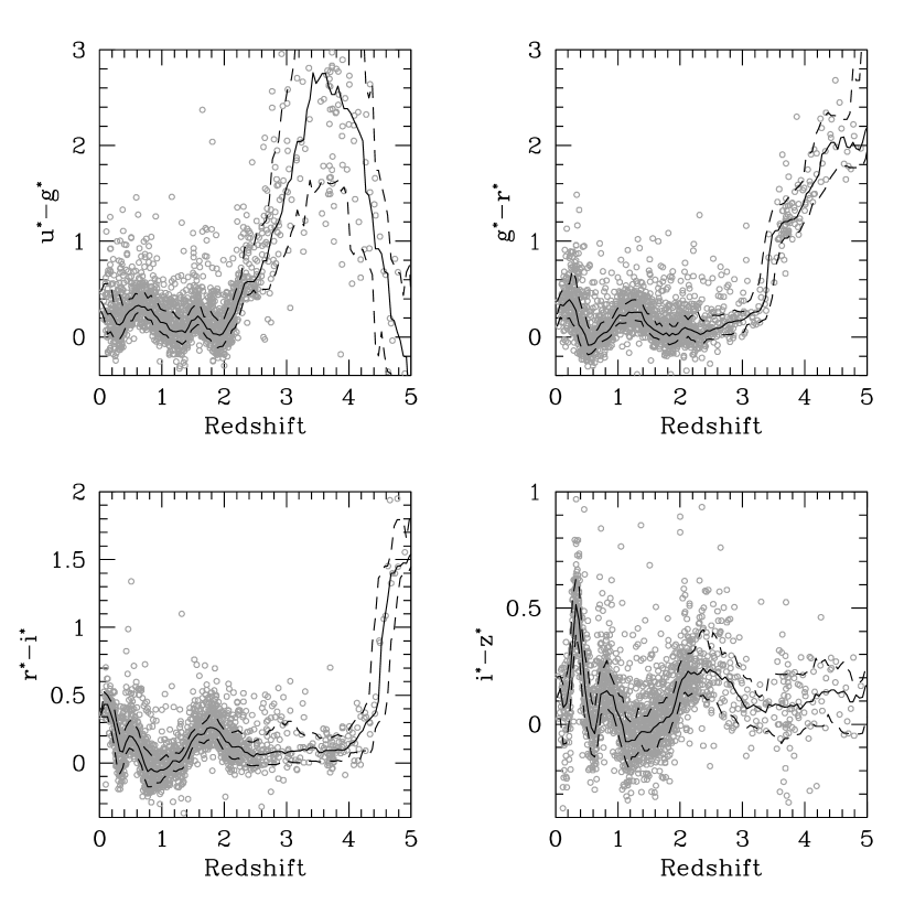
Figure 1: SDSS colors versus redshift for 2625 quasars between $z=0$ and $z=5$ (grey points), the median color as a function of redshift (solid black curve) and the 1-$\sigma$ error width in the color-redshift relation (dashed black curve). [Adapted from R01.]

The SDSS CCD mosaic imaging camera (Gunn et al., 1998) produces accurate ($\leq 0.03$ mag) photometry that makes it possible to discern structure in the quasar color-redshift relation. As can be seen from Figure 1 (adapted from R01), where we plot the measured colors of 2625 quasars (grey points) along with the median color as a function of redshift (solid black curve), the color-redshift relation for quasars in the SDSS filter set shows a relatively tight distribution with a considerable amount of structure. Red outliers are primarily anomalously red quasars (hereafter, referred to as “reddened” quasars, although is it not clear whether they are actually reddened or simply redder than average), which will be discussed in Section 3.2. Also note the sharp changes in color due to absorption by the Lyman-$\alpha$ forest as the quasars move to higher redshifts. With the four colors derived from the five-band SDSS photometry, it is possible to break the degeneracy of the color-redshift relation with sufficient accuracy and efficiency that quasars can be assigned redshifts purely from their colors.

3.1 The $\chi^{2}$ Minimization Technique

As a starting point for our photometric redshift investigation, we begin with one of the simplest methods for determining photometric redshifts given the structure that is seen in Figure 1. First, we construct an empirical color-redshift relation based on the median colors of quasars as a function of redshift. The color-redshift relation was formed by determining the median quasar colors in bins with centers at 0.05 intervals in redshift, and widths of 0.075 for $z\leq 2.15$, 0.5 for $z>2.5$, and 0.2 for $2.15\leq z\leq 2.5$. This relation is based on the assumption that, in our sample, quasars at a given redshift have similar colors; this assumption does not necessarily mean that the restframe color of all quasars should be the same (i.e., there is not necessarily a redshift independent spectral energy distribution). Our empirical color-redshift relation is shown by the solid black line in Figure 1; the colors that encompass 68% of the data in each redshift bin, thus defining an effective $1\sigma$ error width in the color-redshift relation, are given by the dashed black line. The median and error vectors for this data set are also computed in R01 and are given in Table 3 in that paper. Figure 1 contains quasars that were identified by R01 as a population of reddened quasars, which includes objects like Broad Absorption Line (BAL) quasars; these anomalously red objects are removed before computing the median colors as a function of redshift.

Photometric redshifts are then determined by minimizing the $\chi^{2}$ between all four observed colors and the median colors as a function of redshift. All colors are corrected for Galactic reddening according to Schlegel et al. (1998). The $\chi^{2}$ (for each redshift — indicated by the index, “$z$”) is computed as

$$\chi^{2}_{z}=\frac{[(u^{\prime}-g^{\prime})-(u^{\prime}-g^{\prime})_{z}]^{2}}{\sigma_{(u^{\prime}-g^{\prime})}^{2}+\sigma_{(u^{\prime}-g^{\prime})_{z}}^{2}}+C_{gr}+C_{ri}+C_{iz},$$ (1)

where $(u^{\prime}-g^{\prime})$ is the measured $u^{\prime}-g^{\prime}$ color of the object, $(u^{\prime}-g^{\prime})_{z}$ is the color from the median color-redshift relation at a given redshift, $\sigma_{(u^{\prime}-g^{\prime})}$ is the photometric error in the $u^{\prime}-g^{\prime}$ color, which is given by $(\sigma_{u^{\prime}}^{2}+\sigma_{g^{\prime}}^{2})^{1/2}$, and $\sigma_{(u^{\prime}-g^{\prime})_{z}}$ is the $1\sigma$ error width of the median color-redshift relation as a function of redshift. Since the latter term is relatively independent of redshift (see Figure 1), we have chosen to use a fixed value for all redshifts. The terms $C_{gr}$, $C_{ri}$, and $C_{iz}$ are analogous to the term for the $u^{\prime}-g^{\prime}$ colors, but for $g^{\prime}-r^{\prime}$, $r^{\prime}-i^{\prime}$, and $i^{\prime}-z^{\prime}$, respectively. The most probable redshift is given by the redshift that produces the smallest value of $\chi^{2}$. Slightly different formulations of $\chi^{2}$ may be more appropriate depending on certain assumptions, such as whether the width of the color distribution is independent of redshift or if magnitude errors are correlated.

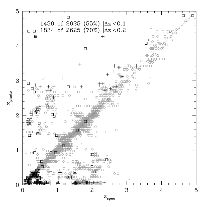
Figure 2: Photometric redshift versus spectroscopic redshift for all quasars in our sample. Points marked with a black cross are anomalously red quasars (see Section 3.2) and boxes indicate extended sources (see Section 3.3).

The first test of this photometric redshift technique is to determine if it can recover the redshifts for the objects that comprise the input data set. The results of such an exercise are shown in Figures 2 to 5, which display the results for the 2625 quasars from R01. In Figure 2, we plot the predicted photometric redshift versus the spectroscopic redshift for all of the quasars in our sample: the same quasars that went into making the empirical color-redshift relation. We find that 1834 of 2625 quasars (or 70%) have photometric redshifts that are correct to within $|\Delta z|=0.2$ or better. The RMS deviations from the correct values are $\Delta_{{\rm all}}=0.676$ and $\Delta_{0.3}=0.099$, where $\Delta_{{\rm all}}$ is the RMS for the whole sample and $\Delta_{0.3}$ is the RMS for those objects whose photometric redshifts are within $|\Delta z|=0.3$ of the spectroscopic redshift. Considering $z>3$ alone, we see that our results are even better than for all redshifts combined. Points marked by crosses are those quasars which are deemed to be anomalously red; they are the points in Figure 1 that lie well above the median relation (see R01 for discussion). Points marked by squares are extended sources; the colors of these objects may be affected by the light from the host galaxy.

Further improvements to our method will come from understanding the distribution of both extended and reddened quasars in addition to investigating inherent redshift degeneracies, all of which are obvious in Figure 2. Sections 3.2, 3.3, and  3.4 are devoted to discussions of how we might reduce the fraction of objects with incorrect photometric redshift estimates. It is also important to realize that all of the objects in our sample are known to be quasars. For actual scientific applications where we know only the colors, obviously not all of the objects will be quasars; this fact must be taken into account in the determination of our efficiency, as we discuss in Section 3.6.

That a solid majority of the quasars have accurate photometric redshifts can be seen more clearly in Figure 3, where we plot a histogram of the differences between the photometric redshifts and the spectroscopic redshifts. This histogram reveals that the photometric redshift error has a relatively Gaussian core with $\sigma\sim 0.1$ that contains $\sim 70$% of the quasars, and “side lobes” at $\Delta z=\pm 1.5$ that each contain about 15% of the objects.

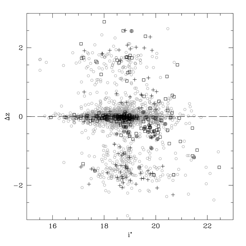
Figure 4: Photometric redshift error ($\Delta z=z_{photo}-z_{spec}$) as a function of SDSS $i^{*}$ magnitude. There is no significant deviation from an average redshift error of zero as a function of magnitude. Plot symbols are the same as for Figure 2.

Figure 4 shows $\Delta z$ as a function of the quasar $i^{*}$ magnitude. That there is no significant deviation from zero as a function of magnitude bodes well for using the photometric redshift technique to estimate redshifts for quasars fainter than the limit of our sample (until the magnitude errors become too large). The potential value of this result for creating a large sample of faint quasars is discussed in Section 3.6.

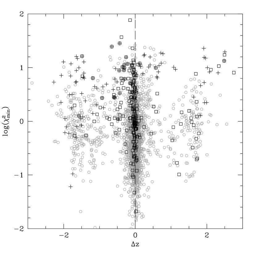
Figure 5: Photometric redshift error ($\Delta z=z_{photo}-z_{spec}$) as a function of minimum $\chi^{2}$. Unfortunately, there is no overall trend toward smaller minimum $\chi^{2}$ with decreasing photometric redshift error. Plot symbols are the same as for Figure 2.

Finally, in Figure 5, we plot $\Delta z$ versus the minimum value of $\chi^{2}$ for each quasar. As long as our photometric errors are relatively small, one would expect the minimum $\chi^{2}$ to decrease with increasing photometric redshift accuracy; if this were true, it would provide an estimate of the accuracy of the photometric redshift. Unfortunately, we see no such trend (except for the very smallest values of $\chi^{2}$). As a result of color degeneracies as a function of redshift, an erroneously predicted redshift can have a small value of $\chi^{2}$. The value of $\chi^{2}$ can be low for more than one redshift, and the lowest $\chi^{2}$ value — which may not be significantly lower than the others — can be associated with an incorrect redshift. See Section 3.4 for a more detailed discussion of redshift degeneracies.

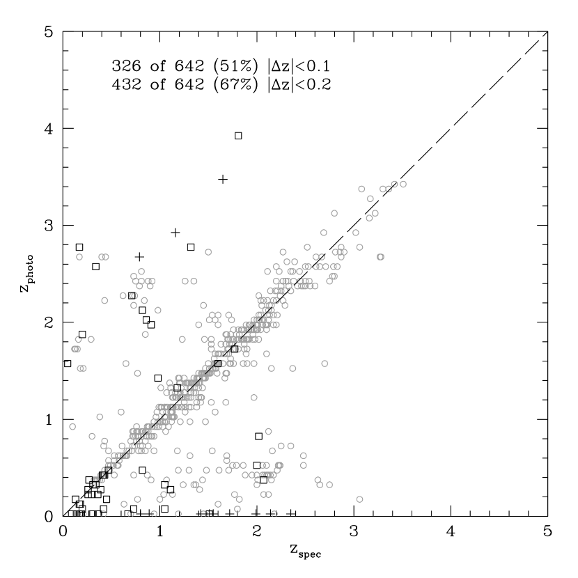
Figure 6: Photometric redshifts versus spectroscopic redshift for NED quasars using only SDSS spectroscopic commissiong quasars to compute the median color-redshift relation. Plot symbols are the same as for Figure 2.

A more challenging test than the analysis presented in Figures 2 to 5 would be to apply this method to a set of quasars that is distinct from the set used to determine the median color-redshift values; Figure 6 shows the results of such an exercise. Here we have calculated photometric redshifts for the subsample of SDSS quasars that were previously known from the NASA Extra-Galactic Database (NED) [see R01 for more details], using a color-redshift relation generated solely from those quasars in our sample that were not previously known to NED. Once again, the photometric redshifts of nearly 70% of the input quasars are correct to within $|\Delta z|=0.2$. The RMS values for this sample are $\Delta_{{\rm all}}=0.702$ and $\Delta_{0.3}=0.105$, essentially identical to the values above. This result is extremely encouraging; one would expect that the accuracy of our initial study (e.g., Figure 1) would be an upper limit to the overall accuracy of the technique and that using independent samples for the median color-redshift relation and the test objects might produce considerably worse results. This is consistent with the statement that the color-redshift relation of quasars is the same for both NED and SDSS quasars. As an additional test, we have also matched the 2dF 10k QSO catalog (Croom et al., 2001) to the SDSS catalog and have determined photometric redshifts for a sample of 2dF quasars using SDSS photometry. We find that 1492 of our 2262 2dF/SDSS matches (all of which have $z<3.2$) have photometric redshifts accurate to within $|\Delta z|=0.2$ — yielding a similar accuracy (66%) to our main sample.

Our results are probably, to some extent, a reflection of how similar the SED’s of quasars are to one another. That quasars are roughly similar can be seen by comparing the quasar composites of Francis et al. (1991), Brotherton et al. (2001), and Vanden Berk et al. (2001), which were made from quasars with different selection criteria, yet are still very similar. Also, if there were a broader distribution of spectral indices and/or emission line strengths, then the color-redshift relation would show much less structure and it would not be possible to determine photometric redshifts for $z<2.2$ quasars. Francis et al. (1992) found that that 75% of the variance in quasar spectra can be accounted for by the first three principal components of their composite spectrum. The first component represents the quasar emission line spectrum, whereas the second component includes the power-law continuum slope and modifications to the emission lines. These two components probably account for nearly all of the structure and the width of the color-redshift relation as shown in Figure 1. As a result of these similarities, quasar photometric redshifts are possible given sufficiently high-quality photometry.

For the sake of comparison, Hatziminaoglou et al. (2000), using two samples of 51 and 46 quasars with photometry from 6 broad-band filters, were able to determine photometric redshifts to within $|\Delta z|<0.1$ for 23 (45%) and 17 (37%) of their quasars in each sample, respectively. Similarly, Wolf et al. (2001) report an accuracy of 50% ($|\Delta z|<0.1$) in their sample of 20 objects using 11 intermediate- and broad-band filters. Our accuracy (fraction of objects within $|\Delta z|<0.2$) is competitive with, if not considerably better than, these previous results using a sample that is more than 50 times as large. Furthermore, it is significant that our study uses only four broad-band colors and that no effort beyond routine SDSS operations is needed to obtain the required measurements.

Thus far, we have applied our algorithm without any pre- or post-processing of the data in the input sample. However, it is clear that an application of some constraints on the input sample will lead to significant improvements in our results without introducing any significant biases. We now turn to a discussion of these techniques.

3.2 Reddened Quasars

Approximately 4% of the quasars in our sample are substantially redder than can be expected from Galactic extinction (R01). Such quasars present a problem for photometric redshift determination, since their colors are significantly different from the intrinsic colors of the average quasar at the same redshift. For example, in Figures 2, 4, 5, and 6 we have marked quasars that are anomalously red for their redshift with black crosses; many of these anomalously red quasars are Broad Absorption Line (BAL) quasars. As one expects, most of the reddened quasars (92%) have incorrect photometric redshifts; moreover, an appreciable fraction (12%) of the quasars with bad photometric redshifts are reddened.

There are a number of ways to deal with reddened quasars to improve the effectiveness of the photo-$z$ algorithm. One could attempt to recognize reddened quasars a priori and apply a correction to their colors. However, this process would only work if the red quasars were clearly identifiable and could be corrected with some sort of global correction factor; such a procedure is unlikely to be very effective due to the broad range of reddening that is observed (the colors of reddened quasars at a given redshift are consistent with the colors of reddened quasars at nearly all other redshifts). One could also attempt to recognize reddened quasars before attempting to calculate their photometric redshifts and then reject them from consideration (as opposed to recognizing them and trying to make a correction).

Identifying red quasars without knowing their redshifts may not be as difficult as it might initially appear. For example, the vast majority of $z<2.2$ quasars have $u^{\prime}-g^{\prime}\leq 0.6$, so a quasar candidate with $u^{\prime}-g^{\prime}>0.6$ is probably either a high-redshift quasar, or a reddened low-redshift quasar (if the object is indeed a quasar). Similar approaches can be tried with outliers in the other colors. Of course, there can be redshift biases inherent in this process: as can be seen in Figure 1, a redshift $1.6$ quasar that is reddened by 0.5 mag stands out more clearly as a red outlier in $u^{\prime}-g^{\prime}$ than does a similarly reddened redshift 1.9 quasar, as a result of the structure in the quasar color-redshift relation.

We have made a preliminary attempt to reject reddened quasars and to study the effects of their rejection on our results. Using only point sources, we have found a series of color-cuts (based initially on the $u^{\prime}-z^{\prime}$ colors) that allow for the identification of reddened quasars that is roughly independent of redshift and unbiased against high-$z$ quasars. These color-cuts are applied uniformly to the entire data set — without the knowledge of the actual redshifts of the quasars. We find that the application of these color-cuts to reject reddened quasars improves our (fractional) success rate to roughly 73%. In order to apply this technique with confidence in the future, we need more than the 40 quasars with $z>4$ that are in our current sample. These additional $z>4$ quasars will determine the empirical scatter in the colors for the highest redshift quasars, which, in turn, will allow a better separation between real high-$z$ quasars and reddened lower redshift quasars.

3.3 Extended Objects

Extended sources, which are plotted as boxes in the figures, pose an additional problem. At high redshift ($z>1$), about half of the quasars which are labeled as extended in the sample presented herein are actually classified as point sources by the latest version of the SDSS image processing software; such objects should not be a problem in the future. However, at low redshift there are low-luminosity objects (Seyferts; see R01) whose colors are likely to be contaminated by the light from the quasar host galaxy and will appear redder than normal. As with the reddened quasars discussed above, we must handle such objects properly to get the best photometric redshifts. At first, it may be wise to simply exclude all extended quasars from our median color-redshift relation and not attempt to determine photometric redshifts for extended sources. After all, it is clear that these have relatively small redshifts (for quasars), which may be sufficient constraint for most science applications. However, in the future, we would hope to be able to determine photometric redshifts for these objects as well.

For our present analysis, we have included extended objects, which has two effects. First, it causes the median colors to be slightly redder at low redshift than they would otherwise be. Second, this means that some extended objects will have quite good photometric redshifts, but that very blue point sources at low redshift might have poorer photometric redshifts than would otherwise be expected. We expect that those extended sources with poor photometric redshifts will tend to have large photometric redshifts, since their redder colors will push them to higher apparent redshifts. A preliminary investigation found that excluding extended objects from the median color-redshift relation does not, in fact, improve our results for point sources; however, more work is needed on the subject.

3.4 Redshift Degeneracies

From Figure 2 it is clear that there are some degeneracies in the color-redshift relation. Such an effect is indicated by outliers that are symmetric around the $z_{spec}=z_{photo}$ line. For example, a number of $z_{spec}\sim 2$ quasars are being assigned photometric redshifts near $0.4$; similarly many $z_{spec}\sim 0.4$ quasars are given photometric redshifts around $2$. To some extent, we may be unable to resolve these degeneracies; however, we have reason to be encouraged that we may be able to determine the correct redshifts for these objects.

In Figure 7, we plot the $\chi^{2}$ (left panels) and the probability density (right panels, see § 3.5.4) as a function of redshift for five sample quasars whose spectroscopic and photometric redshifts disagree by more than $0.2$. Of particular interest is that these objects (that were selected to illustrate the following point) all have local minima at or near the true redshift. As such, it may be possible to assign a second most probable redshift to these objects that is much closer to the true redshift. We find that 331 of 791 objects (42%) whose strongest minima produce erroneous photometric redshifts have the correct redshift as a secondary minimum. If we can find a way to recognize such cases, then our efficiency would improve to about 82%.

We find that, for some objects, the minimum in $\chi^{2}$ for the wrong redshift is narrower than the minimum for the correct redshift (see quasars 4 and 5 in Figure 7). This effect may be due to objects with redshifts near the correct redshift having more similar colors than objects with redshifts near the incorrect redshift. Allowing the algorithm to take the “width” of the minima (i.e., the area under the curve) into account may improve our results. In addition, we note that there are some cases where the minimum is very broad or where there are two closely spaced minima and the photometric redshift estimate is actually quite good (such as for quasar 3 in Figure 7) despite the fact that it is off by more than $0.2$ in redshift.

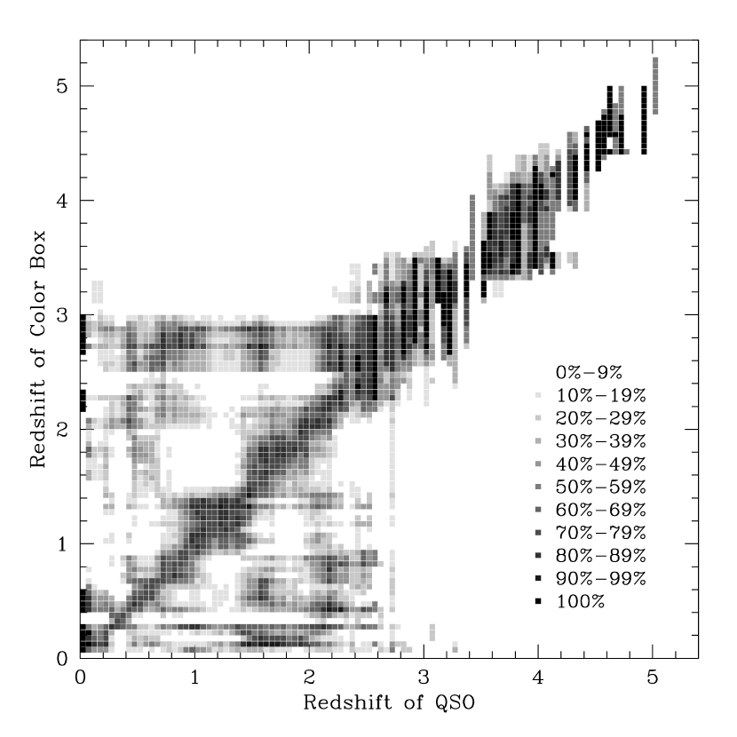
Figure 8: Redshift degeneracy. The grayscale of the pixel at coordinates $(X,Y)$ indicates the fraction of quasars with redshift $X$ which are within the 95% color-box associated with redshift $Y$. (See text for details.)

In order to give the reader an impression for which pairs of redshifts are degenerate in our data, we have created Figure 8. We generate the figure in the following way. First, we calculate the 95% confidence interval about the median in each color, for redshift bins of width 0.05. For each redshift bin, we define a four-dimensional box in color-space, whose lengths along each dimension are the 95% confidence intervals for $u^{\prime}-g^{\prime}$, $g^{\prime}-r^{\prime}$, $r^{\prime}-i^{\prime}$, and $i^{\prime}-z^{\prime}$. These boxes are called the “95% color-boxes”, where “95%” simply refers to the confidence intervals that generated the box; in general, it will not be true that 95% of the quasars in a redshift bin will lie within the color-box associated with that redshift bin.

For the purposes of Figure 8, a quasar is considered to be “consistent” with a certain redshift bin if its position in color-space lies within the 95% color-box for that redshift bin. The shade of gray of the point $(X,Y)$ represents the percentage of quasars in redshift bin $X$ which lie within the 95% color-box of redshift bin $Y$. Note that the fraction in each bin is independent of the other bins; the sum along a column or row can be greater than 100%. One also must keep in mind that some of the redshift bins for $z>2.5$ contain very few ($<10$) quasars, so that the percentages associated with these bins are not always terribly meaningful.

As one would expect, there are high percentages along the “main diagonal” (the line $Y=X$). This just means that most quasars with redshift $X$ are “consistent” with having a redshift of $Y=X$. However, high percentages can also be found at other regions of the figure, for example: at approximately $(2.2,0.4)$, $(1.6,0.2)$, $(1.6,0.7)$, $(2.2,0.7)$, and (to a lesser extent) their symmetric counterparts across the main diagonal; and at a number of regions with $Y\approx 2.8$ and $X<2.8$. These “off-diagonal” redshift pairs are due to the degeneracies in the median color-redshift relation. In some cases these degeneracies may be caused by emission features falling between two filters. For example, $z=0.4$ and $z=2.2$ are somewhat degenerate, perhaps in part because the bulk of the emission from Mg II and Lyman-$\alpha$, respectively, is emitted at wavelengths that fall in the relatively unsensitive region between the $u^{\prime}$ and $g^{\prime}$ filters.

One observes that Figure 8 is not perfectly symmetric about the main diagonal. This is because the two axes are not on equal footing: the $x$-axis deals with the actual distribution of quasars in color-space, while the $y$-axis approximates those distributions (and not very accurately) with the 95% color-boxes. Presumably, Figure 8 would become more symmetric if the color-box for each redshift bin was replaced by a region that more closely resembled the actual distribution in color-space of the quasars belonging to that redshift bin.

In some sense, Figure 8 is a diagnostic for our photometric redshifts. For example, if the photometric redshift of a quasar is around 2.2, we should be aware of the possibility that the spectroscopic redshift is actually near 0.4, since quasars at both redshifts are found in essentially the same region of color-space. Note that, as a result of this diagnostic capability, Figure 8 resembles Figure 2. Knowledge of the degenerate regions of color-space, coupled with other information (such as the expected redshift distribution of the sources) will help to break the redshift degeneracies present in our data and will improve our photometric redshift measurements.

3.5 Future Work

The goal of this paper is not just to describe a photometric redshift algorithm for quasars, but to demonstrate the ability to determine photometric redshifts for quasars using SDSS imaging data — a feat which is significant in and of itself. We are certainly encouraged that our simple photo-$z$ method produces such accurate results; however, the method produces an incorrect redshift about 30% of the time. We have already discussed some specific changes that can be applied to the basic algorithm to improve our efficiency and have shown that it may be possible to increase our efficiency to nearly 85% accuracy. In the following sections, we introduce some less specific and/or more time consuming possibilities for improving our accuracy that are beyond the scope of this paper.

Most importantly, if we are to apply this technique effectively to do real science, we must also be able to select quasars efficiently from their colors alone. Our true accuracy is the efficiency of the quasar color-selection algorithm (roughly 70%) multiplied by our photometric redshift accuracy (roughly 70%), yielding a true accuracy of more like 50%. Thus it is clear that in addition to the need to improve our photometric redshift accuracy, we must also find ways to improve our quasar selection efficiency.

3.5.1 More Data

Clearly as more SDSS imaging data and spectroscopic redshifts are acquired, we can refine our color-redshift relation, which should allow for increased accuracy in determining photometric redshifts — particularly for $z>2.2$ where there are currently very few quasars in each redshift bin. For real $z>2.2$ quasars we already do quite well; however, as we discussed above, additional high-$z$ quasars will help us to discern between lower redshift quasars that are reddened and normal high redshift quasars.

Additional photometric data will allow us to reject more outliers when making the color-redshift relation and will help us to understand how to recognize these outliers — without knowing their spectroscopic redshifts. We will further benefit by being able to better determine the width of the color-redshift relation as a function of redshift and whether that width is purely due to a range of optical spectral indices, or other factors. Better knowledge of the width of the distribution will, in turn, allow for better understanding of what redshifts have color degeneracies. The combination of these improvements in our knowledge may help to improve the accuracy of our photometric redshifts.

3.5.2 More Sophisticated Photo-$z$ Techniques

Since the idea of photometric redshifts has been around for so long (Baum, 1962) and since the technique has been successful using the Hubble Deep Fields (e.g., Sawicki et al., 1997), there is an extensive body of literature that details a number of different techniques from which we might be able to learn (e.g., Baum, 1962; Koo, 1985; Loh & Spillar, 1986; Connolly et al., 1995; Lanzetta et al., 1996; Sawicki et al., 1997; Brunner et al., 1997; Wang et al., 1998; Connolly et al., 1999; Budavári et al., 2000; Csabai et al., 2000). As such, in addition to our simplistic $\chi^{2}$ minimization method, we contemplate the use of other methods that have been tested on galaxies.

In general, traditional galaxy techniques will be difficult to carry over to quasars. Unlike galaxies, the colors of quasars do not occupy a relatively flat plane in color space and a given color does not necessarily correspond to a unique redshift. That is, $z$ is not strictly a function of color. As a result, PCA-type redshift decompositions (Connolly et al., 1995) are probably not possible for quasars (at least in terms of determining photometric redshifts). For high-redshift quasars where the color reddens rapidly as a result of Lyman-$\alpha$ and Lyman-limit absorption, the color-redshift relation is more similar to that of galaxies and traditional galaxy techniques may be more applicable to quasars.

One might, a priori, think that SED-fitting techniques would also be difficult for quasars, since the quasar spectral energy distribution is very close to a power-law: unlike the SED for galaxies. However, in Budavári et al. (2001) we show that quasar photo-$z$ is indeed possible using SED-fitting methods with both a single SED template and a set of four templates. SED-fitting techniques can be helpful when attempting to discriminate between different galaxy spectral types. For quasars, while there are clearly different types of objects (such as Broad Absorption Line QSOs, BL Lacs, etc.), they are not typically divided into spectral types in the same way that galaxies are divided into spectral types. This situation is partially due to a relative dearth of uniform quasar spectra, thus we are hopeful that the situation will change in the near future and that spectral typing of quasars will become more common.

In addition, knowing the apparent magnitudes of the objects is not as useful for quasars as it is for galaxies. For galaxies, the redshift is roughly correlated with apparent magnitude; more distant galaxies tend to be fainter. While it is also true that more distant quasars tend to be fainter than closer quasars, the dynamic range of quasar luminosities is so large that any potentially useful correlation is strongly diluted. However, this does bring up the fact that in using only four colors, we are not using all of the information available, and we are certainly free to add the observed brightness to our equations.

There may be other approaches to be explored that may improve our results. One example would be to use a Bayesian-type analysis (Benítez, 2000), where we would weight our results based on the redshift distribution and/or luminosity function of the quasars in our sample. Such a weighting could help break the degeneracy in cases where two or more photometric redshifts are equally likely. Our initial attempts at using the magnitude distribution as a Bayesian prior suggest that an improvement of 3.5% might be realized by applying this technique.

3.5.3 Infra-red Data

Additional improvements may come from adding infra-red (IR) colors to our analysis; additional colors will contribute to the accuracy of the method. 2MASS (Skrutskie et al., 1997) provides IR imaging data for the entire sky and makes an excellent sample to use for this application. The addition of 2MASS quasars (Barkhouse & Hall, 2001) to our analysis would be very interesting; however, the overlap between the SDSS and 2MASS in magnitude space is limited to the very brightest SDSS quasars (typically, $r^{\prime}\leq 17.5$). Since the SDSS will obtain spectra for all of these objects, this exercise is not as useful as it might otherwise be. Nevertheless, there are applications for such an analysis, but they are beyond the scope of this paper.

3.5.4 Photometric Redshift Probabilities

In addition to finding more than one probable redshift for each object, it would be desirable to give some measure of how confident one can be that the redshift is correct. As a preliminary attempt to assign probabilities to our photometric redshifts, we define the quantity $Ne^{-\chi_{z}^{2}/2}$ to be an estimate of the probability density as a function of redshift for each object, where the value of $N$ normalizes the probability density to unity over the entire redshift range. Examples are given in the right hand panels of Figure 7 where we show the probability density functions for the same quasars as in the left hand panels. This presentation emphasizes the most probable regions of redshift space.

We should also stress that, for some science applications, one will not simply want the most probable redshift. Rather, one might want to know things like “what is the probability that this object really has a redshift larger than X”, or “how likely is it that the correct redshift is other than the most probable redshift”. Clearly, the technique presented herein allows for such applications; work on this subject is in progress.

3.6 Towards One Million Quasars

More than one hundred thousand SDSS quasar candidates brighter than $i^{\prime}\sim 19$ will eventually have SDSS spectra. Clearly, we can also determine photometric redshifts for these quasars; however doing so has limited value since these objects will already have spectroscopic redshifts. The ability to determine photometric redshifts from $u^{\prime},g^{\prime},r^{\prime},i^{\prime},z^{\prime}$ outside of the SDSS survey area will certainly be of interest, but the true value in this method will come from photometric redshift determination of faint objects for which spectroscopic redshifts would require large amounts of telescope time.

In theory, we could determine photometric redshifts for as many as one million quasars in the SDSS area if we can determine photometric redshifts for objects as faint as $g^{\prime}=21$ and if we can select quasar candidates with very high efficiency. We now turn to a discussion of these issues.

3.6.1 Photo-$z$ for Faint Quasars

In principle, we could already determine photometric redshifts for a large sample of faint quasars by using our existing data; however, in practice, it would be better to get more spectra of fainter quasars in order to calibrate the photometric redshifts at the faint end (i.e., to determine whether or not faint quasars have the same intrinsic colors as bright quasars at the same redshift). At least three sources of faint quasar data are possible: 1) the SDSS Southern Survey, where the SDSS will probe to fainter limits that in the Northern Survey, 2) matching SDSS photometry to spectroscopically confirmed quasars from the 2dF QSO Redshift Survey (Croom et al., 2001), and 3) a separate faint quasar follow-up project. To some extent, the need for a test sample of fainter quasars may be moot since we find that the colors of quasars are not a very strong function of luminosity as can be seen in Figure 11 of R01, and because our sample already includes relatively faint quasars.

If the photometric redshift technique can be calibrated out to $g^{\prime}=21$, then we can expect to determine photometric redshifts for as many as one million quasars (Fan, 1999). Can we really estimate redshifts to $21^{\rm st}$ magnitude in the SDSS? It would seem that the answer is “yes”, especially since Figure 4 shows no systematic deviations from zero at fainter magnitudes. That is, this technique is getting incorrect redshifts for as many quasars at fainter magnitudes as it does at the bright end.

The answer also appears to be “yes” from the standpoint of the photometric limits of the imaging Survey. The photometric limit of the Survey in $u^{\prime}$ is approximately 22.3. If we consider only UVX quasars, which have $u^{\prime}-g^{\prime}\leq 0.8$, then this means that we can use this technique to $g^{\prime}=21.5$ (over a magnitude brighter than the Survey limit in $g^{\prime}$). If we cut our sample at $g^{\prime}=21$, then our sample should not be affected by incompleteness in $u^{\prime}$, and the objects will be sufficiently bright that the errors in their magnitudes will not adversely affect our results. Furthermore, we note that the $g^{\prime}=21$ limit applies only to low-redshift quasars. For higher redshift quasars where the Lyman-$\alpha$ forest blocks most of the light from the quasar in one or more of the SDSS filters, photometric redshifts can be determined for fainter quasars.

3.6.2 Efficient Selection of Quasar Candidates

It is important to mention that finding one million quasars requires looking at considerably more than one million quasar candidates; not all SDSS point sources that lie outside of the “stellar locus” are quasars (Richards et al., 2001b). All of the objects used in the analysis of this paper are already known to be quasars. However, in a real photometric redshift application, we will not know if all the objects in the sample are quasars — in fact we will know that many are not quasars. If the SDSS selection efficiency were as high for faint quasars as it is for bright quasars (nearly 70%), then coupled with our 70% accuracy of photometric redshifts, we would expect that only 50% of our proposed faint quasar sample would actually be quasars with the correct photometric redshift. Most science applications will require more than 50% efficiency/accuracy. We have already discussed how we might increase the fraction of correct photo-$z$’s, we now discuss how to increase the efficiency of quasar selection.

Perhaps the easiest way to increase our selection efficiency is to consider only small regions of color space. Without too much difficulty, it should be possible to pick objects from a restricted range of color-space such that the vast majority of objects are quasars. Even a simple UV-excess cut such as $u^{\prime}-g^{\prime}$ $\leq 0.6$ will yield a sample where the majority of point sources will be quasars (if they are sufficiently faint, see Fan 1999). Further color-space restrictions can be used to increase the quasar probability even more (e.g., color cuts to reduce the contamination from white dwarfs — which have SDSS colors that are considerably different from quasars).

Another approach to increase our efficiency is if non-quasars are found to contaminate only certain regions of photometric redshift space. For example, we find that for a sample of 220 white dwarfs, 135 (75%) have photometric redshifts between $1.025$ and $1.225$. If we were to exclude this redshift region from our analysis, we would reduce our contamination from white dwarfs considerably. If other contaminants were similarly confined in photometric redshift space, we might be able to increase our efficiency to a point where the contamination was at an acceptable level. Of course, this method will introduce redshift biases in our analysis, but these biases can be corrected on a statistical basis.

We might also increase the fraction of real quasars in our sample by looking at the radio properties of the sources. Point objects that are radio sources also have a very high probability of being quasars. If we were to restrict our quasar candidate selection to those object that are also FIRST sources, we would improve our quasar selection efficiency considerably, albeit at the cost of a large reduction in sample size.

Full calibration of the photometric redshift technique will require an exploration of most of the color parameter space inhabited by quasars, but individual science applications can take advantage of smaller regions of color space where the quasar fraction is very high. Nevertheless, we are confident that quasars can be selected to sufficient efficiency (or that the efficiency can be modeled accurately) and their photometric redshifts can be determined to sufficient accuracy that good science can be done with such samples. We now turn to a brief discussion of some of these applications.

4 Science Programs with SDSS Quasar Photometric Redshifts

The SDSS quasar sample will represent a factor of 100 increase in the number of quasars from what was recently the largest complete survey in the published literature, specifically the Large Bright Quasar Survey (LBQS; Morris et al. 1991). These 100,000 new SDSS quasars, combined with the 25,000 expected from the 2dF QSO Survey (Boyle et al., 2000; Croom et al., 2001) will yield over a factor of eight increase in the number of spectroscopically confirmed quasars known today. However, if we can successfully calibrate photometric redshifts to $g^{\prime}=21$, we can expect to increase this number by another factor of ten — yielding a million or more quasar candidates with photometric redshifts in the SDSS area. Although not all of the quasar candidates will actually be quasars, as we have discussed above, it should be possible to select subsamples that have a relatively high probability of being quasars.

There are many scientific uses of a such a large statistical sample of quasar candidates with photometric redshifts. Examples of science that will benefit from photometric redshifts of quasar candidates are: quasar-galaxy correlations and amplification bias of quasars (e.g., Thomas et al., 1995; Norman & Impey, 1999), quasar pairs and large scale structure as traced by quasars (e.g., Mortlock et al., 1999; Croom & Shanks, 1996), the luminosity function of faint quasars (e.g., Boyle et al., 2000; Koo & Kron, 1988), and strong gravitational lensing (Richards et al., 1999; Pindor et al., 2000; Mortlock & Webster, 2000).

Quasar amplification bias research can benefit greatly from photometric redshifts of quasars. Current amplification bias studies are limited by small number statistics, since the number of known quasars is actually rather small. A larger sample of quasars would be a significant aid to this research. Contamination of the quasar sample (objects that are not really quasars) merely serves to degrade the amplification bias signal (whether it be a correlation or an anti-correlation with galaxies), making a detection using a photometric redshift sample even more significant.

Strong lensing is another area that is likely to benefit from photometric redshifts. If one were merely attempting to find as many gravitationally lensed quasars as possible, then requiring that pairs of objects have similar photometric redshifts would increase the efficiency of such searches. While the imposition of such a selection criterion would hinder a statistical analysis to determine $\Omega_{\Lambda}$, it would be a very efficient way to find lenses which could be used to determine $H_{\rm o}$.

Quasar-quasar clustering studies also stand to gain from such a photo-$z$ analysis. Even though the SDSS will confirm upwards of $10^{5}$ quasars, quasar-quasar clustering studies require that we take into account the SDSS’s minimum fiber separation limit and the extent to which spectroscopic plates overlap each other. Photometric redshifts of quasars can be used to study clustering to fainter limits and higher density than the spectroscopic survey — without the need for corrections due to spatial selection effects. More importantly, photometric redshifts of quasars will help greatly by increasing the overall density of object that can be used in quasars clustering studies; this is important because of the relative sparseness of bright quasars (as compared to normal galaxies).

Finally we discuss the luminosity function of faint quasars. The photometric redshift technique is not very useful unless it can be used to fainter limits than the spectroscopic part of the Sloan Survey. The calibration of the method fainter than $i^{\prime}=19$ will require an extensive follow-up campaign. Such a calibration sample will be interesting in and of itself. These faint calibration quasars and the eventual faint photo-$z$ quasars can be used to determine the quasar luminosity function at faint limits, which is of great interest in terms of studying the evolution of quasars.

For those programs that are not adversely affected by moderate contamination (i.e., many of the objects really are not quasars) and errors in the redshifts, large regions of color space can be used to select quasar candidates. In this case, the SDSS imaging data can be thought of as an objective prism survey. For more sensitive programs, smaller regions of parameter space (e.g., those that are not contaminated by white dwarfs) can be defined that will give less contamination and more accurate redshifts at the cost of biasing the redshift distribution.

In addition to contamination by non-quasars, redshift errors for real quasars will also need to be accounted for. Although an error in redshift as large as 0.2 may seem large for those who have experience with photometric redshifts of galaxies, for quasars an error of 0.2 is adequate for most science applications. For example, an error of 0.2 is sufficiently small to allow one to split a photo-$z$ sample into “high-redshift” and “low-redshift”. We also emphasize that, to the extent that the photo-$z$ method can be considered low-resolution spectroscopy, a redshift error of $\Delta z=0.2$ is really quite good. For example, at $z=3$ the wavelength error of Lyman-$\alpha$ due to an error in redshift of $\Delta z=0.2$ would only be $243\,{\rm\AA}$, which is smaller than the separation between the Lyman-$\alpha$ and Si IV emission lines.

5 Conclusions

The color-redshift relation of quasars has considerable structure as seen through the SDSS filters. This structure can be used in four dimensions to break the one dimensional degeneracies between quasar colors and their redshifts, and allows for the determination of photometric redshifts, including low-redshift quasars ($z\leq 2.2$). While it is clear that the structure induced by the Lyman-$\alpha$ forest allows for accurate determination of quasar redshifts at large redshift ($z\geq 3.0$), to our knowledge this work, together with Budavári et al. (2001), is the first successful attempt to determine photometric redshifts for a large sample of low-redshift quasars using as few as four broad-band colors.

We can expect at least 70% of the photometric redshifts to be accurate to $|\Delta z|=0.2$ for quasars with $0<z<5$, and this fraction is not apparently a function of magnitude (to at least $i^{\prime}=20$, if not fainter). With a limiting magnitude of $u^{\prime}=22.3$, the SDSS should be able to determine photometric redshifts for quasars brighter than about $g^{\prime}=21.0$, which yields on the order of one million quasar candidates over the entire Survey area. Photometric redshifts for high-redshift quasars can be determined to even fainter limits.

We advocate the construction of a large sample of quasar spectra ($\sim 1000$) fainter than $i^{\prime}=19$ in order to calibrate the photometric relation for magnitudes fainter than the limiting magnitude of the main SDSS quasar survey. The construction of such a sample may allow for the eventual determination of redshifts for a million or more quasar candidates through the photometric redshift techniques described herein. This sample will also be useful for studying the faint end of the quasar luminosity function.

Although one million quasar candidates with photometric redshifts are by no means equivalent to one million quasars with spectroscopic redshifts, there are many scientific topics that can be addressed with such a sample. Some science is relatively insensitive to the quasar selection efficiency and to errors in the redshifts of those objects that are quasars; other programs will require detailed studies of the selection effects and redshift errors in order to take full advantage of the sample. With a bit of effort, it should be possible to create smaller subsamples of the nearly one million quasar candidates that have both a high probablitiy of being a quasar and an accurate photometric redshift. In any case, we expect that there will be no lack of creative uses for the sample of quasar candidates with photometric redshifts that the SDSS will produce.

Figure 3: Histogram of photometric redshift errors ($\Delta z=z_{photo}-z_{spec}$) for the data from Figure 2.

Figure 7: Photometric redshift $\chi^{2}$ (left panels) and probability density (right panels) values as a function of redshift for five quasars with discrepant photometric redshifts. Panels at the same $y$ location (which also have the same number in the lower right hand corner) represent the same quasar. The dashed line denotes the true redshift, whereas the dotted line gives the most probable redshift based on the $\chi^{2}$ minimization.

References

- Barkhouse & Hall (2001) Barkhouse, W. A. & Hall, P. B. 2001, AJ, 121, 2843
- Baum (1962) Baum, W. A. 1962, in IAU Symp. 15: Problems of Extra-Galactic Research, Vol. 15, 390
- Benítez (2000) Benítez, N. 2000, ApJ, 536, 571
- Bessell (1990) Bessell, M. S. 1990, PASP, 102, 1181
- Boyle et al. (2000) Boyle, B. J., Shanks, T., Croom, S. M., Smith, R. J., Miller, L., Loaring, N., & Heymans, C. 2000, MNRAS, 317, 1014
- Brotherton et al. (2001) Brotherton, M. S., Tran, H. D., Becker, R. H., Gregg, M. D., Laurent-Muehleisen, S. A., & White, R. L. 2001, ApJ, 546, 775
- Brunner et al. (1997) Brunner, R. J., Connolly, A. J., Szalay, A. S., & Bershady, M. A. 1997, ApJ, 482, L21
- Budavári et al. (2000) Budavári, T., Szalay, A. S., Connolly, A. J., Csabai, I., & Dickinson, M. 2000, AJ, 120, 1588
- Budavári et al. (2001) Budavári, T., et al. 2001, this volume
- Connolly et al. (1999) Connolly, A. J., Budavári, T., Szalay, A. S., Csabai, I., & Brunner, R. J. 1999, in ASP Conf. Ser. 191: Photometric Redshifts and the Detection of High Redshift Galaxies, ed. M. S. R. J. Weymann, L. J. Storrie-Lombardi & R. J. Brunner (San Francisco: ASP), 13
- Connolly et al. (1995) Connolly, A. J., Csabai, I., Szalay, A. S., Koo, D. C., Kron, R. G., & Munn, J. A. 1995, AJ, 110, 2655
- Croom & Shanks (1996) Croom, S. M. & Shanks, T. 1996, MNRAS, 281, 893
- Croom et al. (2001) Croom, S. M., Smith, R. J., Boyle, B. J., Shanks, T., Loaring, N., Miller, L., & Lewis, I. J. 2001, MNRAS, 322, L29
- Csabai et al. (2000) Csabai, I., Connolly, A. J., Szalay, A. S., & Budavári, T. 2000, AJ, 119, 69
- Fan (1999) Fan, X. 1999, AJ, 117, 2528
- Francis et al. (1992) Francis, P. J., Hewett, P. C., Foltz, C. B., & Chaffee, F. H. 1992, ApJ, 398, 476
- Francis et al. (1991) Francis, P. J., Hewett, P. C., Foltz, C. B., Chaffee, F. H., Weymann, R. J., & Morris, S. L. 1991, ApJ, 373, 465
- Fukugita et al. (1996) Fukugita, M., Ichikawa, T., Gunn, J. E., Doi, M., Shimasaku, K., & Schneider, D. P. 1996, AJ, 111, 1748
- Gunn et al. (1998) Gunn, J. E., et al. 1998, AJ, 116, 3040
- Hatziminaoglou et al. (2000) Hatziminaoglou, E., Mathez, G., & Pelló, R. 2000, A&A, 359, 9
- Koo (1985) Koo, D. C. 1985, AJ, 90, 418
- Koo & Kron (1988) Koo, D. C. & Kron, R. G. 1988, ApJ, 325, 92
- Lanzetta et al. (1996) Lanzetta, K. M., Yahil, A., & Fernandez-Soto, A. 1996, Nature, 381, 759
- Loh & Spillar (1986) Loh, E. D. & Spillar, E. J. 1986, ApJ, 303, 154
- Lupton et al. (1999) Lupton, R. H., Gunn, J. E., & Szalay, A. S. 1999, AJ, 118, 1406
- Morris et al. (1991) Morris et al. 1991, AJ, 102, 1627
- Mortlock & Webster (2000) Mortlock, D. J. & Webster, R. L. 2000, MNRAS, 319, 879
- Mortlock et al. (1999) Mortlock, D. J., Webster, R. L., & Francis, P. J. 1999, MNRAS, 309, 836
- Newberg et al. (2001) Newberg, H., et al. 2001, in preparation
- Norman & Impey (1999) Norman, D. J. & Impey, C. D. 1999, AJ, 118, 613
- Pindor et al. (2000) Pindor, B., et al. 2000, BAAS, 197, 13.06
- Richards et al. (1999) Richards, G. T., et al. 1999, BAAS, 194, 116.03
- Richards et al. (2001a) —. 2001a, AJ, 121, 2308
- Richards et al. (2001b) —. 2001b, in preparation
- Sawicki et al. (1997) Sawicki, M. J., Lin, H., & Yee, H. K. C. 1997, AJ, 113, 1
- Schlegel et al. (1998) Schlegel, D. J., Finkbeiner, D. P., & Davis, M. 1998, ApJ, 500, 525
- Skrutskie et al. (1997) Skrutskie, M. F., et al. 1997, in ASSL Vol. 210: The Impact of Large Scale Near-IR Sky Surveys, 25
- Stoughton et al. (2001) Stoughton, C., et al. 2001, in preparation
- Thomas et al. (1995) Thomas, P. A., Webster, R. L., & Drinkwater, M. J. 1995, MNRAS, 273, 1069
- Vanden Berk et al. (2001) Vanden Berk, D. E., et al. 2001, AJ, in press
- Wang et al. (1998) Wang, Y., Bahcall, N., & Turner, E. L. 1998, AJ, 116, 2081
- Wolf et al. (2001) Wolf, C., et al. 2001, A&A, 365, 681
- York et al. (2000) York, D. G., et al. 2000, AJ, 120, 1579