Long Period Variable Stars: galactic populations and infrared luminosity calibrations.
Abstract
In this paper HIPPARCOS astrometric and kinematic data are used to calibrate both infrared luminosities and kinematical parameters of Long Period Variable stars (LPVs). Individual absolute K and IRAS 12 and 25 luminosities of 800 LPVs are determined and made available in electronic form.
The estimated mean kinematics is analyzed in terms of galactic populations. LPVs are found to belong to galactic populations ranging from the thin disk to the extended disk. An age range and a lower limit of the initial mass is given for stars of each population. A difference of mag in K for the upper limit of the Asymptotic Giant Branch is found between the disk and old disk galactic populations, confirming its dependence on the mass in the main sequence.
LPVs with a thin envelope are distinguished using the estimated mean IRAS luminosities. The level of attraction (in the classification sense) of each group for the usual classifying parameters of LPVs (variability and spectral types) is examined.
Key Words.:
Stars: absolute magnitude – variable stars – kinematics – galactic populations – AGB1 Introduction
Long period variables (LPV) form an important class of red giant stars. They show more or less regular photometric variability with amplitudes reaching up to 8 magnitudes and periods up to 600 days. They traditionally comprise Miras, semi-regular (SR) and irregular (L) variables according to the amplitude and the regularity of their visual light curves. They are known to be either O-rich or C-rich, and comprise thus M, S and C stars. More recently OH-IR sources have been found from infrared and radio observations showing that they belong to the LPV population with periods up to 2000 days. Those sources emit in the infrared and radio wavelengths, and are not associated with any detectable counterpart in optical wavelengths.
The brightest LPVs are luminous enough to be observed at long distances, providing information on the host galaxy, like the Magellanic Clouds (see Van Loon et al., 1999 as an example). While the ranges of masses and ages of LPVs are still the subject of discussion, it is generally accepted that they are large, and are therefore considered as very good tracers of galactic history.
The determination of the characteristics of individual LPVs is usually a
delicate task due to the complexity of the dynamic and chemical
phenomena
to be considered. A statistical study using all available data of a
large sample of LPVs is often needed. A rough example of such an
approach could
be the relation between the mean visual light curves and the infrared
colors of C and O-rich LPVs already presented in Mennessier et al.
(1997a).
In this paper, HIPPARCOS astrometric data and the available
multi-wavelength (K, IRAS 12 and 25) infrared photometric measurements
allow us to calibrate multi-wavelength luminosities and to discriminate
between different galactic populations – and thus different ranges of
initial
masses () – among the LPVs according to their
kinematical
properties. In a second step, individual K and IRAS absolute magnitudes
are estimated for all the 800 considered LPVs using a powerful
statistical
estimator.
Our sample of LPV stars and the data used are described in Sect. 2. The statistical method specifically developed for the study of HIPPARCOS samples is summarized in Sect. 3. Sect. 4 presents the discriminated groups of LPVs resulting from our statistical analysis, while Sect. 5 analyzes the results derived for individual stars. Finally, Sect. 6 reviews the crossed properties derived from the analysis at different wavelengths.
2 The sample of LPV stars
2.1 Data
In order to benefit from the accurate astrometric data made available by the HIPPARCOS satellite, we use in our study the sample of all LPV stars observed on this mission, i.e. the LPVs brighter than 12.5 mag in V during more than 80% of their variability cycle. The sample is composed of about 900 stars which are either of type M (O-rich), C (C-rich) or S (O/C1). They include Mira, SR (of both type a and b) and L variables.
Astrometric data is taken exclusively from the HIPPARCOS Catalogue (Perryman et al. 1997) to provide a homogeneous data set. Radial velocities are taken from the HIPPARCOS Input Catalogue (HIC; Turon et al. 1992).
Photometric data are gathered from various sources. V magnitudes () are taken from the HIC. They correspond to the magnitudes given in the General Catalogue of Variable Stars (GCVS; Kholopov et al. 1985), corrected as described in the HIC volumes to obtain mean magnitudes at the maxima of light. K magnitudes () are taken from the Catalogue of Infrared Observations (Gezari et al. 1996), and include the large set of JHKL measurements of LPVs by Catchpole et al. (1979) and the measurements by Fouqué et al. (1992), Guglielmo et al. (1993), Groenewegen et al. (1993), Whitelock et al. (1994), Fluks et al. (1994), Kerschbaum & Hron (1994), Kerschbaum (1995) and Kerschbaum et al. (1996). Infrared magnitudes are derived from the and fluxes measured at 12 and 25 micrometers respectively by the infrared astronomy satellite (IRAS). We use
| (1) |
and
| (2) |
as given in the IRAS-PSC catalog (vol.1, Sect. VI.C.2). One should note that not all authors use this definition for the infrared magnitudes and . The color index used by Van der Veen and Habing (1988), for instance, is higher than the one deduced from Eqs. 1 and 2 by mag.
Among the 900 stars of our sample, the number of stars for which V, K and IRAS infrared magnitudes are available amounts to 882, 652 and 793, respectively, with 608 stars having both K and IRAS magnitudes.
Finally, variability and spectral types are taken from the GCVS.
2.2 Selection effects
The main selection bias in our sample comes from the HIPPARCOS magnitude limit mag (see Sect. 2.1). This selection is well determined and thus easy to take into account in the statistical analysis.
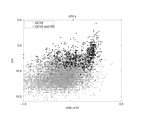
The characteristics of LPVs cause another bias related to the magnitude limit of the sample. LPV stars are evolved red giants, often characterized by the formation of dust around them. The presence of a dusty circumstellar envelope affects the stellar spectrum by reducing their visible light. As a result, obscured LPVs are under-represented in our sample, because the HIPPARCOS selection was done on the basis of the visible magnitude. The importance of this bias can be estimated by comparing the number of stars included in the HIC with the number recorded in the GCVS. This comparison is shown in Fig. 1 as a function of the V magnitude and the color index , where we consider all LPVs of the GCVS for which either the visual () or the photographic () magnitude at maximum is given, and assuming as the mean value for LPVs. All stars from the HIC, represented by filled circles in Fig. 1, are found to have , as expected (the very few exceptions being most probably due to the fact that the assumed relation does not apply to them). Fig. 1 also shows that the number of stars included in the HIC (relative to the number of stars recorded in the GCVS, represented by filled and open circles in Fig. 1) decreases with increasing circumstellar envelope thickness (i.e. decreasing index). This bias is further discussed in Sect. 5.2.3.
It must be noted that the GCVS itself is, of course, not exhaustive, and is certainly biased at the expense of the reddest stars. OH-IR stars, for example, are not well represented in the GCVS sample. For these reasons, a statistical method which can take into account all these biases is necessary for our analysis. This method is described in the next section.
3 The statistical method
In this paper the Luri-Mennessier (LM) statistical method, described in Luri et al. (1996), is used to analyze the sample of LPV stars. The method has been specifically designed to exploit the HIPPARCOS data and thus is suitable for our purposes. This method has already given fruitful results, in particular for Barium stars (Mennessier et al., 1997c), Ap-Bp stars (Gomez et al., 1998) and the LMC distance modulus (Luri et al., 1998).
The use of appropriate statistical methods for the exploitation of the HIPPARCOS astrometric data is crucial in order to obtain correct results. Otherwise the values obtained can be affected by strong biases and the precision of the data will not be fully used. A discussion on the correct use of HIPPARCOS data and recommendations on analysis techniques can be found in Brown et al. (1997).
The LM method used in this paper is especially appropriate for use with the HIPPARCOS data. We refer to Luri et al. (1996) for a detailed description, and only briefly summarize here some of its main features.
First of all, the stellar population from which the sample is extracted is assumed to be composed of several distinct groups. These groups can differ in kinematics, luminosity or spatial distribution and its number is a priori not known. Therefore, using a sample extracted from this base population and taking into account the selection criteria used to create it, the LM method:
-
•
determines the number of significant discriminating groups and the percentage of each of them in the population;
-
•
produces, for each group, unbiased estimates of the parameters of the model used to describe it, i.e.:
-
–
a Schwarzschild ellipsoid velocity distribution characterized by (). and point towards the galactic center, the galactic rotation, and the north galactic pole, respectively;
-
–
an exponential distribution of the number of stars in the direction perpendicular to the galactic plane, with a scale height ;
-
–
a normal distribution of the absolute magnitude in the bandpass of the used observed magnitudes characterized by the parameters and ;
-
–
The results of this first step for our LPVs sample are given in Sect.
The minimum input data needed by the LM method are the measured positions, proper motions and apparent magnitudes of the stars, but it can also use the parallaxes and radial velocities if available. The method takes into account the selection effects of the sample, the observational errors, the galactic rotation and the interstellar absorption.
In a second step, once the groups are identified and parametrized, the method:
-
•
computes for each star of the sample, the a posteriori probability that the star belongs to a given group;
-
•
uses a Bayesian rule to assign each star to a group;
-
•
uses a statistical estimator to obtain estimations of individual distances and luminosities for each star.
This second step is presented in Sect. 5 where the representativity of our sample with respect to the kinematic and photometric properties of the population is also discussed.
4 Calibrations of the LPVs population
The LM method was applied four times, as described in Sect. 3, once for each photometric bandpass: V – results already presented in Mennessier et al. (1997b) –, K, 12 and 25 – in the present paper. In principle, one could assign a joint luminosity distribution to two or more bandpass magnitudes simultaneously, and the LM method would separate the sample into stellar groups consistent with all the photometric measurements together. This option, however, requires a perfectly well known relationship between the different magnitudes in order to define a joint distribution function as realistic as possible for all the band passes. The correlation between the near-infrared (K) and IRAS infrared properties presently cannot be well modeled and very likely has a non-unique form depending on the stellar and circumstellar evolutive stage along the AGB. Thus, we decided not to couple the photometric band passes and to calibrate each luminosity separately. Furthermore, bandpasses are related to different physical processes and can provide separate interesting information: V is greatly affected by absorption molecular lines, K reflects the stellar emission, and IRAS bandpasses depend on the nature and density of grains in the circumstellar envelope.
The LM method is simultaneously sensitive to kinematics and luminosity and thus the number of significant discriminating groups depends on both these characteristics and is not necessarily the same for the different bandpass analyses. Furthermore, the samples used are not the same, and this can also affect the number of discriminated groups.
Six distinct groups are identified in the V magnitudes, three in K and four in each of the two IRAS magnitudes. Those are successively analyzed in terms of the classical galactic populations. Although the number of groups is found to be different for each analysis, the groups present similarities in their kinematical composition and with respect to the galactic populations (see sect. 6).
4.1 The V band
An analysis of the six groups identified in the V band has been presented in Mennessier et al. (1997b). In order to compare these results with the ones obtained for infrared calibrations, the main results are summarized here. Table 1 reviews the estimated mean parameters for the analysis corresponding to the V luminosity at the phase of maximum light. The LPVs are found to belong to all galactic populations from disk to very extended disk. We wish to emphasize three points:
-
•
LPVs belonging to the bright disk population (BD) have a mean luminosity of =-3.6 and =104pc, while the corresponding values for the disk population (D) are =-1.0 and =126pc. Among LPVs belonging to BD population there are probably stars at the upper limit of the AGB or even at the first step of the post-AGB state.
-
•
the main group (44) has an estimated scale height of =249pc. Its kinematics is typical of the old disk population.
-
•
a few LPVs (less than 2) belong to the extreme extended disk (ED), with greater than 1200pc and a very large Schwarzschild ellipsoid velocity distribution. This most probably indicates a birth of those stars early in the evolution of our Galaxy. Those stars should thus be a metal-deficient disk population (see 6.2). This is consistent with the bright luminosity found (=-2.8).
| Group | BD | D | OD1 | OD2 | TD | ED |
|---|---|---|---|---|---|---|
| -3.6 | -1.0 | -1.2 | -0.2 | -1.2 | -2.8 | |
| 1.4 | 0.8 | 0.2 | 1.0 | 0.5 | 1.2 | |
| -10 | -6 | -44 | -1 | -34 | -61 | |
| -11 | -6 | -35 | -21 | -84 | -235 | |
| -13 | -6 | -6 | -10 | -19 | -20 | |
| 13 | 24 | 28 | 37 | 77 | 188 | |
| 14 | 14 | 25 | 23 | 29 | 126 | |
| 9 | 9 | 22 | 23 | 65 | 72 | |
| 104 | 126 | 217 | 249 | 409 | 1227 | |
| 8 | 25 | 13 | 44 | 8 | 2 |
4.2 The K band
Only three groups are identified in the K band. From their kinematics and spatial distribution, given in Table 2, they can be interpreted as the galactic disk (D), old disk (OD) and extended disk (ED) populations. They are similar to the four main groups identified in the V band (Sect. 4.1), except that the disk and a part of the old disk population seem to be mixed.
In a previous analysis of a sample restricted to O-rich Miras (Alvarez et al.,1997), only two groups were found. One corresponded to the extended disk population, with a percentage of 17, in agreement with our result i.e. 18/142=13 of O-rich Miras belonging to the ED group (see table 7). The other group mixed disk and old disk populations. In the present paper, a more numerous sample allows a more refined separation of the kinematic populations.
| Group D | Group OD | Group ED | ||||
|---|---|---|---|---|---|---|
| est. | est. | est. | ||||
| -6.1 | 0.4 | -6.0 | 0.7 | -5.3 | 0.8 | |
| 1.1 | 0.3 | 0.7 | 0.4 | 1.4 | 0.5 | |
| -7 | 10 | -17 | 27 | -21 | 14 | |
| 29 | 9 | 45 | 16 | 111 | 11 | |
| -12 | 8 | -36 | 25 | -123 | 12 | |
| 16 | 5 | 27 | 11 | 69 | 18 | |
| -9 | 6 | -6 | 9 | -20 | 19 | |
| 12 | 3 | 26 | 13 | 90 | 25 | |
| 184 | 44 | 268 | 85 | 782 | 313 | |
| 60 | 35 | 5 | ||||
| Group D | Group ODb | Group ODf | Group ED | |||||
|---|---|---|---|---|---|---|---|---|
| est. | est. | est. | est. | |||||
| -6.4 | 0.3 | -8.0 | 0.4 | -6.4 | 0.5 | -6.2 | 1.0 | |
| 1.7 | 0.1 | 1.2 | 0.2 | 0.6 | 0.4 | 1.6 | 0.2 | |
| -6 | 9 | -12 | 5 | -10 | 9 | -30 | 37 | |
| 22 | 6 | 35 | 8 | 39 | 6 | 106 | 45 | |
| -7 | 8 | -26 | 7 | -24 | 8 | -97 | 54 | |
| 12 | 5 | 26 | 11 | 22 | 6 | 65 | 64 | |
| -9 | 4 | -9 | 5 | -8 | 5 | -2 | 44 | |
| 9 | 8 | 21 | 8 | 21 | 7 | 75 | 29 | |
| 161 | 55 | 258 | 56 | 256 | 79 | 1065 | 724 | |
| 29 | 32 | 29 | 10 | |||||
| Group D | Group ODb | Group ODf | Group ED | |||||
|---|---|---|---|---|---|---|---|---|
| est. | est. | est. | est. | |||||
| -7.1 | 0.5 | -8.6 | 0.4 | -6.5 | 0.3 | -6.8 | 0.8 | |
| 1.7 | 0.1 | 1.2 | 0.2 | 0.6 | 0.4 | 1.6 | 0.5 | |
| -6 | 6 | -10 | 4 | -10 | 7 | -39 | 48 | |
| 21 | 8 | 36 | 10 | 38 | 6 | 111 | 33 | |
| -6 | 4 | -26 | 7 | -22 | 6 | -99 | 63 | |
| 13 | 4 | 27 | 9 | 22 | 5 | 69 | 23 | |
| -10 | 4 | -9 | 5 | -8 | 4 | 1 | 42 | |
| 11 | 7 | 21 | 8 | 20 | 4 | 75 | 37 | |
| 158 | 43 | 277 | 34 | 270 | 107 | 1610 | 1180 | |
| 28 | 32 | 30 | 10 | |||||
4.3 The IRAS bands
The four LPV groups identified in the IRAS 12 and 25 bands are given in Tables 3 and 4, respectively. They are similar to those identified in the K band (Table 2), except that the old disk group is further divided into “bright” (ODb) and “faint” (ODf) subgroups. Let us remember here that the method allows us to distinguish groups with similar mean kinematics but different luminosities (ODb and ODf) or groups with a similar luminosity distribution but different kinematics (D and ED for instance). Moreover, it is important to remark that D, ODb and ED have, on average, a similar color index mag corresponding to a thick circumstellar envelope, while ODf has a mean index of 0.1 mag that suggests that the majority of the stars in this last group have thin envelopes.
Let us finally point out that the kinematic parameters () associated with each of the four groups are very similar for both the 12 and 25 calibrations.
5 Individual estimates and properties of the sample


5.1 Individual estimates
Once the parameter estimation and group discrimination is completed, each star in our initial sample is a posteriori attributed to one of the LPV groups identified in each bandpass, following the method described in Sect. 3. This allows us to estimate the most probable individual distance and absolute magnitude in each band according to the observed astrometric, kinematic and photometric data and attributed group.
Due to the probabilistic nature of the Bayesian procedure, some misclassification is unavoidable. To check and improve individual star assignations in each wavelength, we compare the calculated color indices (obtained from the estimated individual absolute magnitudes deduced by the Bayesian assignations in the and/or wavelengths) with the observed color indices (). 5% of the stars are re-assigned to groups reducing the differences for their indices 25-12 and/or K-12.
Figure 2 shows the histograms of difference of for the indices 25-12 and K-12 of all the stars in the sample. These distributions are related to the errors of the individual estimated luminosities and of the observed magnitudes. We can deduce that the accuracies of our estimated individual luminosities are distributed according to a gaussian rule of standard error 0.3 mag. and 0.1 mag. respectively in K and IRAS bands. The lower accuracy in the IRAS bands is consistent with the fact that IRAS photometry is more homogeneous than the K photometry, and that the variability amplitude of LPVs is smaller in the IRAS bands than in K. As previously stated, the LM method has allowed us to take advantage of all the available information, leading to better estimations of the individual absolute magnitudes. Furthermore, the LM method has provided at the same time the statistical distribution of these individual magnitudes (see Sect. 3 and 4). The individual estimates of K, 12 and 25 luminosities are given in a table available in electronic form at the CDS 111via anonymous ftp to cdsarc.u-strasbg.fr (130.79.128.5) or via http://cdsweb.u-strasbg.fr/cgi-bin/qcat?J/A+A/ and are included in the specialized ASTRID database 222via http://astrid.graal.univ-montp2.fr.
5.2 Comparison of sample/population
The LM method gives unbiased calibrations for the base population. It also gives individual kinematic and photometric estimates for each star of the sample. The distribution of these individual estimates (Sect. 5.1) is, of course, biased by the sample selection criteria, contrary to the group characteristics derived in Sect. 4. A comparison of the statistical properties of the sample with the calibrated parameters for the population allows us to check the representativity or the bias of the sample with respect to the population.
5.2.1 Kinematic representativity
Let us analyze the representativity of our sample stars with respect
to the kinematics. The observed proper motions and radial velocities,
together with the estimated individual distances, allow us to compute
the three velocity components and the distance above the
galactic plane for each star in our sample. The mean kinematical
properties of our sample derived from these individual estimates are
shown in Table 5 for each group of the K and 12 bands.
They are very similar to the parameters describing the groups
(Tables 2 and 3), showing that our
sample is very representative of the LPVs population as far as the
kinematics is concerned.
This conclusion was expected since there is a priori no selection affecting (directly or indirectly) the kinematics of our sample and thus no bias is introduced in the kinematics of the stars. We can also note that the proportion of the different groups in the sample is close to that found in the population.
5.2.2 Luminosity representativity


Although no kinematical bias is introduced when selecting a sample
with a cut in apparent magnitude, it is well known that a bias in
luminosity is introduced. Figure 3 shows the
histograms of the individual absolute magnitudes of the stars in our sample
in each group of the K and IRAS bandpasses, together with the normal
unbiased distributions estimated by the LM method for the population.
These distributions are in units normalized to the surface of
each histogram -and not to the number of
population stars in each sample -, thus
only the relative shapes and the magnitude shifts of both
histogram and unbiased distribution are relevant.
The bias of our sample towards higher luminosities is very clear both
in K and IRAS bands. In the IRAS bands, the under-representativity of
faint stars in our sample is more pronounced for LPV stars in the disk
group than in the other IRAS groups. This corresponds to the classical
Malmquist bias (1936), increasing with increased
value. In short, the under-representation of faint stars in our
sample is important for the K or IRAS faint stars and even more for
the disk population, specially in the case of IRAS bandpasses.
However, let us remark that the brightest stars in every group of the sample coincide with the brightest luminosity of the group base population.
| K | ||||
|---|---|---|---|---|
| D | OD | ED | ||
| -13 | -31 | -121 | ||
| 30 | 41 | 111 | ||
| 18 | 27 | 62 | ||
| 20 | 26 | 84 | ||
| 185 | 245 | 621 | ||
| N | 396 | 224 | 39 | |
| % | 60 | 34 | 6 | |
| 12 | ||||
| D | ODb | ODf | ED | |
| -7 | -28 | -20 | -105 | |
| 20 | 42 | 35 | 110 | |
| 14 | 27 | 22 | 66 | |
| 12 | 39 | 21 | 77 | |
| 152 | 343 | 180 | 714 | |
| N | 239 | 273 | 231 | 51 |
| % | 30 | 34 | 29 | 7 |
5.2.3 Envelope effects and representativity
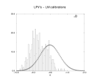
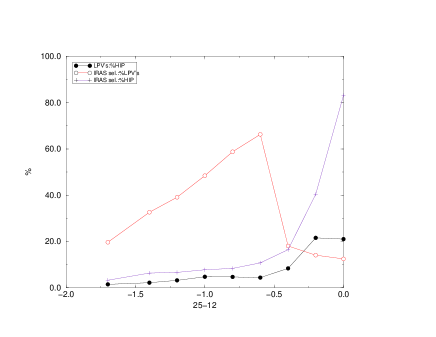
The luminosity sampling bias is not independent of the existence, thickness and composition of a circumstellar envelope around LPVs. Figure 4, which shows the percentage of known LPVs measured by HIPPARCOS (LPVs:%HIP) as a function of the IRAS (25-12) color index, shows that the incompleteness depends on the IRAS color. This is not surprising because the thicker the envelope, the fainter the star in the visual wavelengths.
This is confirmed if instead of using the known LPVs we use the IRAS
sources with a (25-12) color index compatible with the LPVs values of
this index. In doing so, we include stars in the LPV region not
necessarily classified as variables (IRAS sel.:%LPVs). The bias of
the HIPPARCOS sample is more strongly dependent on the envelope
thickness if we do the comparison with these selected IRAS sources.
Thus the percentage of stars observed by HIPPARCOS (IRAS sel.:%HIP)
strongly and abruptly increases up to 80 % for 25-12 decreasing to
zero.
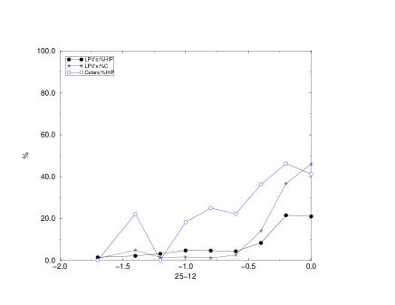
Finally, figure 5 shows how much the sample of carbon-rich stars measured by HIPPARCOS (C stars:%HIP) does not represents either the percentage of the C-rich stars among the known LPVs (LPVs:%C stars) or the percentage of stars known as LPVs measured by HIPPARCOS (LPVs:%HIP). Thus one should be careful about making any interpretation from the percentages of C-rich stars, as we will see in sect. 6.4 .
6 Properties of crossed groups
6.1 Crossing K and IRAS
Due to the difficulties coming from the large uncertainties on :
large amplitudes and variations from one cycle to another, the V
results will not be further used in our analysis and we will
concentrate on the K and IRAS results.
The luminosity estimations in the K and IRAS bands complement each other in the sense that, in general, K fluxes characterize stellar properties while IRAS fluxes provide information on the circumstellar envelope. Thus, the most physically interesting results are obviously obtained by simultaneously considering K and IRAS luminosities. We have already seen that it is very difficult to calibrate these luminosities at the same time due to the incomplete knowledge and non-uniqueness of the relation between the different magnitudes (Sect. 3). Another possibility is to do a crossing of the groups from both the K and IRAS calibrations i.e. to examine the properties of the stars belonging to the same group in K and IRAS.
The first remarkable result concerns the number of crossed groups: only 7 are not empty while 12 could, a priori, be expected. Interestingly, there is no mixture of the extended disk group (in either wavelength) with any other group, except two stars (O-rich SRa: RW Eri and O-rich Mira: SV And), which is compatible with the statistical classification errors. This is a nice confirmation of the power of the LM method to extract consistently distinct groups in biased samples of a given stellar population.
| Disk1 | Disk2 | Old Disk | Ext. Disk | ||||
| D(D) | OD(D) | D(ODf) | D(ODb) | OD(ODf) | OD(ODb) | ED(ED) | |
| nb of stars | 141 | 21 | 103 | 90 | 81 | 113 | 36 |
| -6 | -7 | -18 | -19 | -34 | -32 | -123 | |
| 23 | 28 | 35 | 36 | 42 | 40 | 114 | |
| 13 | 23 | 20 | 18 | 24 | 26 | 63 | |
| 11 | 11 | 34 | 16 | 21 | 29 | 80 | |
| 166 | 191 | 208 | 231 | 160 | 310 | 620 | |
| age range | 1-4 yr | 4-8 yr | 8-gt10 yr | ||||
| lower mass limit | 2-1.4 | 1.4-1.15 | 1.15-lt1 | ||||
Table 6 gives the number of stars in our sample which
are assigned to every crossed group G(G’) i.e. to group G in K and G’
in IRAS. In Sect.5.2.1 our LPVs sample is shown to be
representative of the LPVs population as far as the kinematics is
concerned. Thus the mean kinematics of the stars belonging to a
crossing group K(IRAS) may be considered as representative of the mean
kinematics of the LPVs population belonging to this group.
Obviously such a consideration does not apply to the luminosities (see Sect.5.2.2). The assigned groups are given in annex A (electronic table).
6.2 Ages and initial masses
Table 6 gives the values of the axes of the velocity
ellipsoids and the scale height of each of the 7 crossed K and IRAS
groups. Given that our sample is representative of the population in
terms of kinematics, as already seen in Sect. 5.2.1, we
can use the kinematical values of table 6 as
representative in terms of galactic populations.
The relation between the mean kinematics of a galactic population and its age allows us to estimate the range of ages of the groups. Furthermore, classical statistical studies of stars known to belong to different galactic populations and of different metallicity abundances allow us to add an estimate of the range of metallicity. By comparing the values in table 6 with the results on kinematics and metallicity of the galactic populations by Mihalas and Binney (1981) and by Stromgren (1987), we can deduce:
-
•
D(D) and OD(D) populations are 1-4 yr old with a solar metallicity. Part of the stars in D(D) are classified as belonging to the bright disk population (BD) by the V analysis, being younger and with a small over-abundance.
-
•
The age of D(ODf) and D(ODb) populations can be estimated to be in the range 4-8 yr, with a metallicity from the solar one to [Fe/H] around -0.4 i.e. Z between 0.006 and 0.02.
-
•
OD(ODf) and OD(ODb) populations are composed of stars older than 8 yr, up to more than yr, with [Fe/H] from the solar value to -0.7 i.e. Z between 0.004 and 0.02
-
•
Stars classified as belonging to ED are probably very old and deficient with [Fe/H] between -0.7 and -1.5 i.e. Z of the order of (0.001,0.004).
Moreover, we can estimate initial masses from evolutionary tracks. From Binney and Merrfield (1998) we can estimate a lower limit of the initial mass of a given age star that has reached the AGB. Thus, values of 2, 1.4, 1.15, 1 can be deduced as lower limits of of the stars of solar metallicity of respectively 1, 4, 8, 12 yr. This agrees with the results on the ages at the top of the early-AGB (Charbonnel et al.,1996).
All these results are in the same ranges as the ones given by Jura and Kleinmann (1992), but our classification is more refined because it is not based on the spectral types and periods which are now known to not really be discriminative parameters for LPVs.
6.3 Evolutionary tracks
Figure 6 shows the K magnitude as a function of the V-K color index for each of the disk1, disk2, old disk and extended disk groups. For comparison, evolutionary AGB model predictions are also shown for three different masses (1.5, 2.5 and ) at solar metallicity, and at three different metallicities (Z=0.004, 0.008 and 0.02) for stars. These models have been computed at Geneva, and are described in Mowlavi (1999) and Mowlavi & Meynet (2000). The conversion between model variables (effective temperature and luminosity ) to observable quantities ( and ) was done by using the transformations given by Ridgway et al. (1980).
Several uncertainties affect both model predictions and the color transformation relations for AGB stars (which are characterized by peculiar chemical compositions as a result of dredge-up episodes). They also affect the determination of the stellar V magnitudes as noted in Sect. 4.1. Thus, the comparison between the evolutionary tracks and the distributions of our sample stars in each group shown in Fig. 6 can only provide qualitative results.
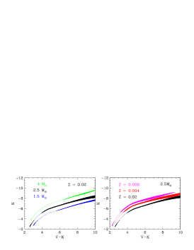
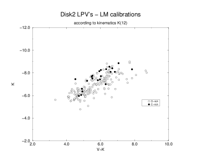
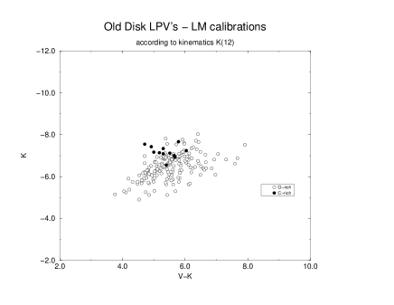
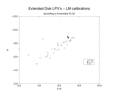
Evolutionary tracks show that, at a given metallicity, stellar luminosities increase with initial stellar mass (at a given V-K). We thus conclude, at least qualitatively and due to the solar or slightly deficient abundance of the majority of HIPPARCOS stars, that our sample stars have lower mass limits which respectively decrease as we consider disk1, disk2 and old disk groups. This is in agreement with the conclusions drawn in Sect. 6.2. Stars of the extended disk group, on the other hand, are compatible with lower metallicities, given their higher K luminosities.
We note that the evolutionary tracks cannot, even if freed from any uncertainty, attribute a single (M,Z) set of parameters to a star because of the degeneracy of those two parameters. A higher luminosity in K at a given V-K could be either attributed to a higher initial mass or lower metallicity. Kinematics can help in distinguishing such ambiguous cases.
Finally, we can comment on the smaller V-K values for the bright disk LPVs. This confirms the strong circumstellar absorption in V for these massive stars.
6.4 Variability and spectral types
The composition of each crossed group K(IRAS) with respect to usual classifications of LPVs (variability and spectral types) is given by the contingency table of both assignations (Table 7). The associated attraction-repulsion indices (Tenenhaus, 1994) – ratio of the observed frequency to the theoretical frequency in the case of independence of both modalities – are more significant in characterizing the correspondence analysis of types and of groups. These indices are given in Table attract or repel each other if the attraction-repulsion index is larger or smaller than 1 respectively.
| L-C | SRb-C | SRa-C | M-C | L-O | SRb-O | SRa-O | M-O | |
|---|---|---|---|---|---|---|---|---|
| D(D) | 29 | 25 | 7 | 9 | 20 | 29 | 4 | 31 |
| OD(D) | 1 | 3 | 0 | 1 | 1 | 4 | 1 | 9 |
| D(ODb) | 7 | 3 | 1 | 4 | 6 | 33 | 7 | 28 |
| D(ODf) | 2 | 4 | 0 | 2 | 42 | 39 | 3 | 2 |
| OD(ODf) | 3 | 5 | 0 | 1 | 34 | 22 | 2 | 0 |
| OD(ODb) | 0 | 3 | 0 | 0 | 14 | 28 | 13 | 54 |
| ED(ED) | 1 | 1 | 0 | 1 | 4 | 7 | 3 | 18 |
| L-C | SRb-C | SRa-C | M-C | L-O | SRb-O | SRa-O | M-O | ||
|---|---|---|---|---|---|---|---|---|---|
| Disk1 | D(D) | 2.7 | 2.3 | 3.5 | 2.0 | 0.6 | 0.7 | 0.4 | 0.9 |
| Disk1 | OD(D) | 0.7 | 1.4 | 0 | 1.6 | 0 | 0.9 | 0.9 | 1.9 |
| Disk2 | D(ODb) | 0.3 | 0.5 | 0.8 | 1.5 | 0.3 | 1.4 | 1.4 | 1.4 |
| Disk2 | D(ODf) | 0.3 | 0.6 | 0 | 0.7 | 2.3 | 1.5 | 0.6 | 0.1 |
| Old Disk | OD(ODf) | 0.6 | 1.1 | 0 | 0.5 | 2.5 | 1.2 | 0.4 | 0 |
| Old Disk | OD(ODb) | 0 | 0.4 | 0 | 0 | 0.6 | 0.9 | 2.2 | 2.1 |
| Ext. Disk | ED(ED) | 0.4 | 0.4 | 0 | 0.9 | 0.6 | 0.7 | 1.6 | 2.2 |
¿From Table 8 we can deduce that:
-
•
The groups corresponding to initially less massive stars are essentially attractive for O-rich LPVs and the ones corresponding to initially massive stars are essentially attractive for C-rich LPVs.
-
•
The strong attraction of C-rich stars by groups corresponding to more massive initial stars is clear. It agrees with the results already given by V calibration (Mennessier et al., 1999) and with both observations and model predictions according to which dredge-up of carbon from core to the surface of AGB stars is more efficient in massive stars (Dopita et al.,1997). However, we must be very cautions. Indeed, the biases described before (section 5.2.3) show the over-representativity of C-rich stars in the sample and the large number of missing LPVs. To which galactic population do the not-HIPPARCOS-observed LPVs belong? Are they O or C-rich? The ratio of carbon to oxygen-rich LPVs that goes up to 78% for the D(D) sample could be due to the sampling. Thus deduced implications for the dependence on the mass of the efficiency of the dredge-up are to be taken with caution.
-
•
O-rich SRa’s are distributed close to O-rich Miras.
-
•
O-rich SRb’s are significantly present in the two disk population groups. The first one is composed of stars without a shell or with a thin one (cf sect.4.3). This probably corresponds to early AGB stars with a relatively high initial mass. The second one contains stars with a shell and corresponds to stars in the same stage as SRa and Miras. This agrees with results by Kerschbaum and Hron (1992). O-rich irregular LPVs are close to the SRb’s lacking a shell and are probably early AGB stars.
-
•
The difference between L irregular variable stars according to their spectral type is evident. C-rich L stars correspond to massive TP-AGB’s with a thick envelope. On the contrary, O-rich L stars are close to early AGB O-rich SRb’s but their initial mass range seems to be more extended to lower masses.
-
•
One CH star (V Ari) is assigned to the Extended Disk population and it is the faintest star in all the luminosities. This completely agrees with the usual hypothesis considering this type of star as an old giant star. Its amplitude of variability is less than 1 magnitude, a very small value even for a semi-regular. The C character of this type of star is however difficult to explain. HIPPARCOS observations suggest that V Ari could be a suspected multiple star but this is not conclusive.
6.5 Upper limit of the AGB
In Section 5.2.2 we remarked that the brightest stars in the sample agree with the brightest luminosity for each group population (see figure 3). Thus we can consider our sample as representative of the LPVs population as far as the brightest luminosities are concerned. Our calibrations show that the upper limit in K luminosity of the OD population ( mag.) is fainter than that of the D population ( mag.) as seen in Table 2. This confirms the dependence of the upper limit of the AGB on . Willson (1980) has described a schematic evolution on the AGB related to the mass-loss rate, its acceleration by the pulsations and probably the induced dust formation. She found a difference in solar luminosities of where stars of solar abundance and equal to 1.5 and 1 leave the AGB. Our result is of the same order.
7 Conclusion
Using available HIPPARCOS data we apply the LM algorithm to improve
the luminosity calibrations in visible, near-infrared and infrared
wavelength ranges and to get information about the star and the
circumstellar envelope.
According to the galactic population – related to initial mass and
metallicity of the stars – and to the circumstellar envelope
thickness and expansion, several groups of LPVs are obtained: bright
(BD) and disk (disk1) galactic population with bright and expanding
envelope, not so young and massive disk population (disk2) divided
into 2 groups: one with thin envelope (f) and the other with a bright
and expanding envelope (b). A similar separation according to envelope
properties is found for the old disk (OD) population. At least some
LPVs are found to belong to extended disk (ED) population.
Our results deduced from kinematic properties confirm that the AGB
evolution depends on the initial mass of the progenitor in the main
sequence. This agrees with the comparison of color-magnitude diagrams
using
our estimated individual luminosities with theoretical evolutionary
tracks. According to the assigned galactic population we can give
ranges of age and of the lower limit main sequence mass for each star of
our sample. The upper limit of the AGB also depends on . The difference of the values
found in K luminosity limits are consistent
with Willson’s schematic model related to the mass loss rate and its
acceleration by the pulsations: ”Stars evolve up the AGB with only
moderate mass loss; at Mira pulsation commences,
driving the mass loss rate up by at least a factor 10”.
The induced dust formation is followed
by the stabilization of the K luminosity after the carbon enrichment.
The ultimate aim of this work is to estimate individual K, 12 and 25
absolute magnitudes given, in the annex (available as an electronic
table at CDS and in the ASTRID database). This allows us to study
simultaneously the stellar properties and the
behavior of the circumstellar envelope. The results recalled in the
previous paragraph are obtained thanks to the estimated individual
luminosities and they mainly concern properties related to the
assigned galactic populations. They will be systematically used in
another paper (Mennessier et al., 2001) to study implications regarding the
physics of LPVs, specifically the simultaneous stellar and
circumstellar evolutions along the Asymptotic Giant Branch.
Acknowledgements.
This work is supported by the PICASSO program PICS 348 and by the CICYT under contract ESP97-1803 and AYA2000-0937. We thank A.Gomez for fruitful discussions of our first results.References
- (1) Alvarez, R., Mennessier, M.O., Barthès, D., Luri, X., Mattei J.A., 1997, A&A 327, 656
- (2) Binney, J., Merrfield, M., 1998, Galactic Astronomy, Princeton Univ. Press Ed.
- (3) Brown A.G.A., Arenou F., Leeuwen F., Lindgren L., Luri X., 1997, ESA SP-402, 63
- (4) Catchpole R.M., Robertson B.S.C., Lloyd Evans T.H.H., Feast M.W., Glass I.S., Carter B.S., 1979, SAAO Circ. 1, 61
- (5) Charbonnel C., Meynet G., Maeder A., Schaerer D., 1996, A&AS 115,339
- (6) Dopita M.A., Vassiliadis E., Wood P.R., et al., 1997, ApJ 474, 188
- (7) Fluks M.A., Plez B., Thé P.S., de Winter D., Westerlund B.E., Steenman H.C., 1994, A&AS 105, 311
- (8) Fouqué P., Le Bertre T., Epchtein N., Guglielmo F., Kerschbaum F., 1992, A&AS 93, 151
- (9) Gezari D.Y., Pitts P.S., Schmitz M., Mead J.M., 1996, Catalogue of Infrared Observations (edition 3.5), available from VizieR at CDS
- (10) Groenewegen M.A.T., De Jong T., Baas F., 1993, A&AS 101, 513
- (11) Gomez, A., Luri, X., Grenier, S., Figueras, F., North, P., Royer, F., Torra, J., Mennessier, M.O., 1998, A&A 336, 953
- (12) Guglielmo F., Epchtein N., Le Bertre T., Fouqué P., Hron J., Kerschbaum F., Lepine J.R.D., 1993, A&AS 99, 31
- (13) Jura, M., Kleinmann, S.G., 1992, ApJS 79, 105
- (14) Kerschbaum F., 1995, A&AS 113, 441
- (15) Kerschbaum, F., Hron, J., 1992, A&A 263, 97
- (16) Kerschbaum F., Hron J., 1994, A&AS 106, 397
- (17) Kerschbaum F., Lazaro C., Habison P., 1996, A&AS 118, 397
- (18) Kholopov P.N., et al., 1985, General Catalogue of Variable Stars, 4th ed. (Moscow: Moscow Pub. House)
- (19) Luri X., Mennessier M.O., Torra J., Figueras F., 1996, A&AS 117, 405
- (20) Luri, X., Gomez, A., Torra, J., Figueras, F., Mennessier, M.O. ,1998, A&A 335, 81
- (21) Malmquist K.J., 1936, Stockholms Obs. Medd. No 26
- (22) Mennessier, M.O., Boughaleb H., Mattei J.A., 1997, A&AS 124, 1
- (23) Mennessier, M.O., Mattei J.A., Luri, X., 1997, New aspects of LPVs from HIPPARCOS. In: HIPPARCOS Venice’97. ESA-SP402 p.275
- (24) Mennessier, M.O., Luri, X., Figueras, F., Gomez, A.E., Grenier, S., Torra, J., North, P., 1997, A&A 326, 722
- (25) Mennessier, M.O., Alvarez, R., Luri, X., Noirhomme-Fraiture M., Rouard, E., 1999, Physics and evolution of LPVs from HIPPARCOS kinematics. In: Le Bertre T., Lèbre A., Waelkens C. (eds) AGB stars. IAU Symposium 191, p. 117
- (26) Mennessier, M.O., Luri, X., 2001, A&A, submitted
- (27) Mihalas, D., Binney, J., 1968, Galactic Astronomy, Freeman Ed.
- (28) Mowlavi N., 1999, A&A 350, 73
- (29) Mowlavi N., Meynet G., 2000, A&A, 361,959
- (30) Perryman M., and the HIPPARCOS science team, 1997, ESA, 1997, The HIPPARCOS Catalogue, ESA SP-1200
- (31) Rydgway S.T., Joyce R.R., White N.M., Wing R.F., 1980, ApJ 235, 126
- (32) Stromgren, B., 1987 In: Gilmore G. and Carswell B. (eds) The Galaxy, NATO ASI Series C Vol. 207, p. 229
- (33) Tenenhaus, M., 1994, Methodes statistiques en gestion, Dunod Ed.
- (34) Turon C., Crézé M., Egret D., et al., 1992, The HIPPARCOS Input Catalogue, ESA SP-1136
- (35) van der Veen W., Habing, H.J., 1988, A&A 195, 125
- (36) van Loon, J. Th., Groenewegen, M. A. T., de Koter, A., et al., 1999, A&A 351, 559
- (37) Whitelock P., Menzies J., Feast M. et al., 1994, MNRAS 267, 711
- (38) Willson L.A., 1980, Miras, mass loss and the origin of Planetary nebulae In: Effects of Mass loss on Stellar Evolution, IAU Coll. 59