Gravitational lensing constraint on the cosmic equation of state

Abstract

Recent redshift-distance measurements of Type Ia supernovae (SNe Ia) at cosmological distances suggest that two-third of the energy density of the universe is dominated by dark energy component with an effective negative pressure. This dark energy component is described by the equation of state $p_{x}=w\rho_{x}$ $(w\geq-1)$. We use gravitational lensing statistics to constrain the equation of state of this dark energy. We use $n(\Delta\theta)$, image separation distribution function of lensed quasars, as a tool to probe $w$. We find that for the observed range of $\Omega_{m}\sim 0.2-0.4$, $w$ should lie between $-0.8\leq w\leq-0.4$ in order to have five lensed quasars in a sample of 867 optical quasars. This limit is highly sensitive to lens and Schechter parameters and evolution of galaxies.

1 Introduction

Recent redshift-distance measurements of SNe Ia at cosmological distances suggest that $2/3$ of the energy density of the universe could be in the form of a dark energy component with an effective negative pressure [1, 2, 3, 4]. This causes the universe to accelerate. There is other observational evidence which also supports the existence of an unknown component of energy density with pressure $p=w\rho$. This includes the recent measurements of the angular power spectrum which peak at $l\sim 200$ [5] and the dynamical estimates of the matter density $\Omega_{m}=0.35\pm 0.07$ [6]. Many candidates have been proposed for this dark energy component which is characterised by an equation of state $-1\leq w\equiv p/\rho\leq 0$.

The first candidate is the cosmological constant characterised by $\omega=-1$. In this case the vacuum energy density or the $\Lambda-\mathrm{term}\;(8\pi G\rho_{vac})$ is independent of time ( for a recent review see [7]). There are several other possibilities for this dark energy:

1. A time varying $\Lambda-\mathrm{term}$[8]

2. Rolling scalar fields (quintessence)[9]

3. Frustrated network of topological defects in which $w=-N/3$ where N is dimension of the defect [10].

4. X-matter [11]

There are some independent methods for constraining $w$. For example Perlmutter et al. (1999) obtained $w<-0.6$ (95% CL) using large-scale structure and SNe Ia in a flat universe [2]. Waga & Miceli (1999) used lensing statistics and supernovae data to find that $w<-0.7$ (68% CL) in a flat universe [12]. Recently, Lima & Alcaniz (2000) used age measurements of old high redshift galaxies (OHRG) to limit $w$ [13]. In flat universe for $\Omega_{m}=0.3$, the ages of OHRG give $w\leq-0.27$. By combining the “cosmic concordance” method with maximum likelihood estimator, Wang et al. (2000) found that the best-fit model lies in the range $\Omega_{m}=0.33\pm 0.05$ with an effective equation of state $w\sim-0.6\pm 0.07$ [14].

In this work we model this unknown form of dark energy as X-matter which is characterized by its equation of state, $p_{x}=w_{x}\;\rho_{x}$ and $w_{x}\geq-1$. We use gravitational lensing as a tool to constrain the $w$ for X-matter. In section 2 we describe some formulae (age-redshift relationship and angular diameter distance) used in lensing statistics. In section 3 we explain the use of $n(\Delta\theta)$, the image separation distribution function of lensed quasars, as a tool to constrain the cosmic equation of state of dark energy. We summarize our results in sec. 4.

2 Cosmology with dark energy

We consider spatially flat, homogeneous and isotropic cosmologies. The Einstein equations in the presence of nonrelativistic matter and dark energy are given by:

$$H^{2}(z)\,\equiv\,({\dot{R}\over R})^{2}\;=\;H_{0}^{2}\left[\Omega_{m}\,({R_{0}\over R})^{3}+\Omega_{x}\,({R_{0}\over R})^{3(1+w)}\right]$$ (1)

$$({\ddot{R}\over R})={-1\over 2}H_{0}^{2}\left[\Omega_{m}\,({R_{0}\over R})^{3}+(1+3w)\;\;\Omega_{x}\,({R_{0}\over R})^{3(1+w)}\right]$$ (2)

where the dot represents derivative with respect to time. Further

$$\Omega_{m}={8\;\pi\;G\over 3H_{0}^{2}}\rho_{m0}\;\;,\;\Omega_{x}={8\;\pi\;G\over 3H_{0}^{2}}\rho_{x0}$$

where $H_{0}$ is the Hubble constant at the present epoch, while $\rho_{m0}\;\;{\rm{and}}\;\;\rho_{x0}$ are the nonrelativistic matter density and the dark energy density respectively at the present epoch. For more details see ref.[15].

The age of the universe at the redshift z is given by

$$H_{0}\;t(z) = H_{0}\;\int_{z}^{\infty}{dz^{\prime}\over(1+z^{\prime})H(z^{\prime})}$$ (3)

$$=\int_{z}^{\infty}{dz^{\prime}\over(1+z^{\prime})\sqrt{\Omega_{m}(1+z^{\prime})^{3}+\Omega_{x}(1+z^{\prime})^{3(1+w)}}}.$$

The angular diameter distance between redshifts $z_{1}$ and $z_{2}$ reads as

$$d_{A}(z_{1},z_{2})={R_{0}\over(1+z_{2})}\int_{z_{1}}^{z_{2}}{dz\over\sqrt{\Omega_{m}(1+z)^{3}+\Omega_{x}(1+z)^{3(1+w)}}}.$$ (4)

3 $n(\Delta\theta)$ as a probe

$n(\Delta\theta)$ is the image separation distribution function for lensed quasars. To understand $n(\Delta\theta)$ we first have to calculate the optical depth. The lensing probability or the optical depth $d\tau$ of a beam encountering a lensing galaxy at redshift $z_{L}$ in traversing $dz_{L}$ is given by the ratio of the differential light travel distance $cdt$ to its mean free path between successive encounters with galaxies $(1/n_{L}(z)\sigma)$, $n_{L}(z)$ is the number density of galaxies and $\sigma$ is the effective cross-section for strong lensing events. Therefore,

$$d\tau=n_{L}(z)\sigma{cdt\over dz_{L}}dz_{L}.$$ (5)

We further assume it to be conserved: $n_{L}(z)=n_{0}(1+z_{L})^{3}$. The present-day galaxy luminosity function can be described by the Schechter function [16]

$$\Phi(L,z=0)dL\,=\,\phi_{\ast}\,\left({L\over L_{\ast}}\right)^{\alpha}\,\,\exp\left(-{L\over L_{\ast}}\right)\,{dL\over L_{\ast}}.$$ (6)

The present day comoving number density of galaxies can be calculated as

$$n_{0}=\int_{0}^{\infty}\Phi(L)dL.$$ (7)

The Singular Isothermal Sphere (SIS) model with one dimensional velocity dispersion $v$ is a good approximation to account for the lensing properties of a real galaxy. The deflection angle for all impact parameters is given by $\hat{\alpha}=4\pi v^{2}/c^{2}$. The lens produces two images if the angular position of the source is less than the critical angle $\beta_{cr}$, which is the deflection of a beam passing at any radius through an SIS:

$$\beta_{cr}=\hat{\alpha}D_{LS}/D_{OS},$$ (8)

We use the notation $D_{OL}=d_{A}(0,z_{L}),\,D_{LS}=d_{A}(z_{L},z_{S}),\,D_{OS}=d_{A}(0,z_{S})$.

Then the critical impact parameter is defined by $a_{cr}=D_{OL}\beta_{cr}$ and the cross-section is given by

$$\sigma=\pi a_{cr}^{2}=16{\pi}^{3}\left({v\over c}\right)^{4}\left({D_{OL}D_{LS}\over D_{OS}}\right)^{2}.$$ (9)

The differential probability $d\tau$ of a lensing event can be written as

$${d\tau\over dz_{L}}=n_{L}(z)\left[{16\pi^{3}\over{cH_{0}^{3}}}v^{4}\,\left({D_{OL}D_{LS}\over R_{0}D_{OS}}\right)^{2}\,{1\over R_{0}}\right]{cdt\over dz_{L}}dz_{L}.$$ (10)

The total optical depth can be obtained by integrating $d\tau$ from $0$ to $z_{S}$ which is equal to [17]

$$\tau(z_{S})={F^{*}\over 30}({D_{OS}(1+z_{S})})^{3}(R_{0})^{-3}$$ (11)

with

$$F^{*}={16\pi^{3}\over{cH_{0}^{3}}}\,\phi_{\ast}\,v_{\ast}^{4}\Gamma\left(\alpha+{4\over\gamma}+1\right).$$

We neglect the contribution of spirals as lenses as their velocity dispersion is small as compared to ellipticals. The relationship between the luminosity and velocity is given by the Faber-Jackson relationship ${\frac{L}{L_{*}}}=\left({\frac{v}{v_{*}}}\right)^{\gamma}$. Table 1 lists lens and Schechter parameters as given by Loveday et al. [18] (hereafter LPEM parameters) and Kochanek [17] (hereafter K96 parameters). For most of our calculations we use LPEM parameters unless specified otherwise.

The differential optical depth of lensing in traversing $dz_{L}$ with angular separation between $\phi$ and $\phi+d\phi$ is given by [19]:

$${\frac{d^{2}\tau}{dz_{L}d\phi}}\,{d\phi}\,{dz_{L}} = {{{\gamma}/{2}}\over\phi}\left[{D_{OS}\over{D_{LS}}}\phi\right]^{{\frac{\gamma}{2}}(\alpha+1+{\frac{4}{\gamma}})}\exp\left[-\,\left({D_{OS}\over{D_{LS}}}\phi\right)^{\frac{\gamma}{2}}\right]{c\,dt\over dz_{L}}$$ (12)

$$\times\,F^{*}\,{(1+z_{L})^{3}\over\Gamma\left(\alpha+{4\over\gamma}+1\right)}\left[\,\left({D_{OL}D_{LS}\over R_{0}D_{OS}}\right)^{2}\,{1\over R_{0}}\right]\,{d\phi}\,{dz_{L}}$$

The normalized image angular separation distribution for a source at $z_{S}$ is obtained by integrating the above expression over $z_{L}$:

$${d{\mathcal{P}}\over d\phi}\,=\,{1\over\tau(z_{S})}\int_{0}^{z_{s}}\,{\frac{d^{2}\tau}{dz_{L}d\phi}}{dz_{L}}.$$ (13)

We include two correction factors in the probability of lensing: (1) the magnification bias and (2) the selection function due to finite resolution and dynamic range.

The magnification bias $B$ is an enhancement of the probability that a quasar is lensed. The bias for a quasar at redshift $z$ with apparent magnitude $m$ is written as

$$B(m,A_{1},A_{2},z)=({dN\over dm})^{-1}{\int_{A_{1}}^{A_{2}}{dN\over dm}(m+2.5\,logA,z)\,\,p(A)dA}$$ (14)

where $p(A)$ is the probability distribution for a greater amplification $A$ which is $8/A^{3}$ for SIS model. We use $A_{1}=2$ and $A_{2}=10^{4}$. We use the quasar luminosity function as given by Kochanek [17],

$${dN\over dm}\propto\left(10^{-x(m-m_{0}(z))}+10^{-y(m-m_{0}(z))}\right)^{-1}$$ (15)

where

$${\rm m_{0}}\;(z)=\left\{\begin{array}[]{lll}m_{0}+(z+1)&{\rm if}&z<1\\ m_{0}&{\rm if}&1<z<3\\ m_{0}-0.7(z-3)&{\rm if}&z>3.\end{array}\right.$$

We use $x=1.07$, $y=0.27$ and $m_{0}=18.92$. We considered a total of 862 $(z>1)$ highly luminous optical quasars plus five lenses [12].

Selection effects are caused by limitations on dynamic range, limitations on resolution and presence of confusing sources such as stars. Therefore we must include a selection function to correct the probabilities. In the SIS model the selection function is modeled by the maximum magnitude difference $\Delta m(\theta)$ that can be detected for two images separated by $\Delta\theta$. This is equivalent to a limit on the flux ratio $(f>1)$ between two images $f=10^{0.4\,\Delta m(\theta)}$. The total magnification of images becomes $A_{f}=A_{0}(f+1)/(f-1)$. So the survey can only detect lenses with magnifications larger than $A_{f}$. This sets a lower limit on the magnification. Therefore, $A_{1}$ in the bias function gets replaced by $A_{f}(\theta)$. To get selection function corrected probabilities we divide our sample into two parts: the ground based surveys and the HST Snapshot survey. We use the selection function as suggested by Kochanek [20]. The corrected image separation distribution function for a single source at redshift $z_{S}$ is given as [17, 21]

$$P(\Delta\theta)\, = \,B(m,A_{f}(\theta),A_{2},z){{{\gamma}/{2}}\over\phi}\int_{0}^{z_{S}}\left[{D_{OS}\over{D_{LS}}}\phi\right]^{{\frac{\gamma}{2}}(\alpha+1+{\frac{4}{\gamma}})}\exp\left[-\,\left({D_{OS}\over{D_{LS}}}\phi\right)^{\frac{\gamma}{2}}\right]$$ (16)

$$\times\,F^{*}\,{cdt\over dz_{L}}{(1+z_{L})^{3}\over\Gamma\left(\alpha+{4\over\gamma}+1\right)}\left[\,\left({D_{OL}D_{LS}\over R_{0}D_{OS}}\right)^{2}\,{1\over R_{0}}\right]\,\,{dz_{L}}.$$

Similarly the corrected lensing probability for a given source at redshift $z$ is given as [17, 21]

$$P=\,\int{d{\mathcal{P}}\over d\phi}B(m,A_{f}(\theta),A_{2},z)\;d\phi.$$ (17)

Here $\phi$ and ${\Delta\theta}$ are linked through $\phi={\frac{\Delta\theta}{8\pi(v^{*}/c)^{2}}}$.

The expected number of lensed quasars is $n_{\rm L}=\sum P_{i}$, where $P_{i}$ is the lensing probability of the ith quasar and the sum is over the entire quasar sample. Similarly, the image-separation distribution function for the adopted quasar sample is $n(\Delta\theta)=\sum P_{i}(\Delta\theta)$. The summation is over all quasars in a given sample.

4 Results and Discussions

Gravitational lensing statistics is a sensitive cosmological probe for determination of the nature of dark energy. This is because statistics of multiply imaged lensed quasars can probe the universe to a redshift $z\sim 1$ or even higher. This is the time when dark energy starts playing a dominant role in the dynamics of universe.

That lensing statistics can be used as a tool to constrain various dark energy candidates has been known for some time. Kochanek (1996) gave a $2\sigma$ upper bound on $\Omega_{\Lambda}<0.66$ from multiple images of lensed quasars[17]. Waga & Miceli (1999) used the combined analysis of gravitational lensing and Type Ia supernovae to constrain the time dependent cosmological term [12]. Their combined analysis shows that $w\leq-0.7$. Cooray and Huterer (1999) also used lensing statistics to constrain various quintessence models [22]. However, there are several uncertainities involved in using gravitational lensing statistics as a tool to probe cosmology [14].

In this article we neglect the role of spirals as lenses as their velocity dispersion is small as compared to E/S0 galaxies. The constraints obtained from lensing statistics strongly depend on lens parameters. There is a need for updated Schechter parameters, the faint end slope $\alpha$ and normalisation $\phi_{*}$ for E/S0 galaxies. Earlier work on lensing statistics used $\alpha\sim-1$, which implies the existence of numerous faint E/S0 galaxies acting as lenses. Because of limited resolution, this faint part of the luminosity function is still uncertain. Also the parameters should be determined in a highly correlated manner from a galaxy survey and use of parameters derived from various surveys might introduce error. We use the updated luminosity function of LPEM. The LPEM luminosity function is characterised by the shallow slope $\alpha$ at faint end and the smaller normalisation $\phi_{*}$ which shifts the distribution to large image separations [21]. Fig. 1 shows the expected number of lensed quasars $n(\Delta\theta\leq 4^{\prime\prime})$ as a function of $\Omega_{m}$ in a flat universe with $w=-1$ for the LPEM and K96 [17] lens and Schechter parameters (see Table 1). We observe K96 parameters predict more lensed quasars for this sample and for no value of the parameter $\Omega_{m}$ the expected number of lensed quasars becomes equal to 5. Moreover, as pointed out by Chiba et al. [21] K96 parameters have been derived from various galaxy surveys and hence lack consistency.

Recently several galaxy surveys have come up with a much larger sample of galaxies. This has improved our knowledge of the galaxy luminosity function. But these surveys don’t classify the galaxies by their morphological type [23]. In lensing statistics we need Schechter parameters of early type galaxies only. We feel at the moment LPEM survey provides the most complete information regarding the early type galaxies.

We use the image separation distribution function function $n(\Delta\theta)$ to constrain the cosmic equation of state for the dark energy. $n(\Delta\theta)$ depends upon $w$ through the angular diameter distances as shown in Section 2. By varying $w$, the distribution function changes which on comparison with the observations gives a constraint on $w$.

Fig.1 shows the expected number of lensed quasars $n(\Delta\theta\leq 4^{\prime\prime})$ as a function of $\Omega_{m}$ in a flat universe with $w=-1$. Comparing the predicted numbers with the observed lenses, we find a value of $\Omega_{m}=0.45$. We further generate $10^{4}$ data sets (quasar sample) using the bootstrap method. We find ’best fit’ $\Omega_{m}$ for each set to obtain error bars on $\Omega_{m}$. We finally obtain $\Omega_{m}=0.5\pm 0.2$. Therefore the gravitational lensing statistics do not favour a large cosmological constant.

In Fig.2 $n(\Delta\theta)$ is plotted against $\Delta\theta$ (image separation) in the flat cosmology for various values of $w$. The plotted rectangles indicate the image-separation distribution of the five lensed quasars in the optical sample considered in this calculation. As indicated by recent distance measurements of Type Ia supernovae, we fix $\Omega_{m}=0.3$ in Fig. 2. On comparing the theoretical prediction of image distribution function with the observations we see that $w=-1$ predicts a large number of lenses which is not supported by the observations. On the other hand, $w=0$ gives too few lensed quasars. We also plot the expected image seperation distribution for $w=-0.7$ and $w=-0.5$ (which corresponds to point (-0.5,0.3) on the curve in Fig. 3). Unfortunately, we cannot do a statistical study here as the number of lensed quasars in this sample is only five.

If we increase the value of $\Omega_{m}$ in a flat universe, a smaller value of $w$ is required to match with observations. The magnitude of the peak $n(\Delta\theta)$ is sensitive to the value of $\Omega_{m}$ in a flat universe. A larger value of $\Omega_{m}$ for a fixed value of $z$ gives a smaller angular diameter distance and hence a smaller value of the peak. The position of the peak of $n(\Delta\theta)$ is sensitive to the value of $\alpha$ i.e. the faint end slope of the luminosity function. If we take the conventional value of $\alpha=-1$, the peak will shift to a lower value of $\Delta\theta$ or in other words it will predict lensed images with smaller angular separations[24].

In Fig. 3 we show the $\Omega_{m}$-$w$ plane. Each point on the curve corresponds to a pair of $(\Omega_{m},w)$ for which the expected number of lensed quasar is equal to five ($n_{\rm L}=5$). If the matter contribution $\Omega_{m}$ increases, a smaller value of $w$ is required to produce five lenses. The dotted lines in this figure correspond to the observed range $\Omega_{m}\sim 0.2-0.4$ [25]. The corresponding range for $w$ in the flat universe is $-0.8\leq w\leq-0.4$. These results agree very well with the limit obtained on $w$ by other independent methods as described in the introduction. With this range of $w$ we can rule out atleast two dark energy candidates. First, cosmic strings $(w\sim-0.33)$ and second the cosmological constant $(w=-1.0)$. It is quite interesting to compare this result with the limit obtained on $w$ by using the MAXIMA-1 AND BOOMERANG-98 data. This data treats the dark energy as a quintessence giving a limit $-1\leq w\leq-0.5$. Our constraint on $w$ is much tighter than that obtained by using the MAXIMA-1 AND BOOMERANG-98 [26].

The constraints obtained here depend strongly on lens and Schechter parameters, evolution of galaxies and, of course, on the quality of the lensing data. The dependence of $n(\Delta\theta)$ on lens and Schechter parameters (as shown in eq.(12) comes mainly through $F^{*}$ (eq.11), exponential dependence on $\gamma$ and other related factors present in the expression for the differential optical depth in traversing distance $dz_{L}$ and with angular separation $d\phi$. The presence of galaxy evolution decreases the optical depth and hence the constraint on $w$ becomes weaker [27]. The main difficulty is that the number of observed lensed QSOs in this sample is too small to put strong constraints on $w$. Extended surveys are required to establish $n(\Delta\theta)$ as a powerful tool. The upcoming Sloan Digital Sky Survey which is going down to $1\sigma$ magnitude limit of $\sim 23$ will definitely increase our understanding of lensing phenomena and cosmological parameters. Moreover, a large number of new gravitational lens systems $(\sim 18)$ have been discovered by the Cosmic Lens All-Sky Survey (CLASS)[28, 29]. CLASS is the largest survey of its kind which has more than 10000 radio sources down to a 5 GHz flux density of 30 mJy. But the major disadvantage of a radio lens survey is that there is little information on the redshift-dependent number-magnitude relation. This may lead to serious systematic uncertainties in the derived cosmological constraints.

We need a larger and complete sample of high-z QSOs, a better understanding of the formation and evolution of galaxies over wide range of redshifts and accurate luminosity function parameters before any definitive and strong statements can be made regarding the constraints on $w$ by gravitational lensing.

$Survey$	$\alpha$	$\gamma$	$v^{*}(Km/s)$	$\phi^{*}(Mpc^{-3})$	$F^{*}$
$LPEM$	$+0.2$	$4.0$	$205$	$3.2\times 10^{-3}$	$0.010$
$K96$	$-1.0$	$4.0$	$225$	$6.1\times 10^{-3}$	$0.026$

Table 1: Lens and Schechter parameters for E/S0 galaxies.

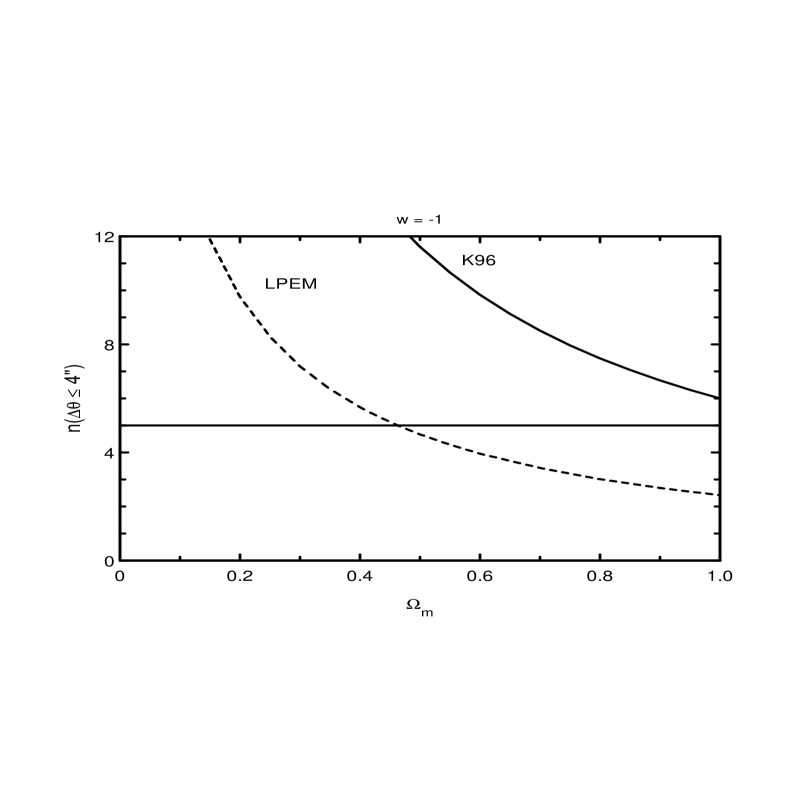
Figure 1: Predicted total number of lenses with $\Delta\theta\leq 4^{\prime\prime}$ as function of $\Omega_{m}$ for flat universe with $w=-1$ (constant $\Lambda$). The observed five lensed QSOs from optical lens survey is shown by horizantal line.

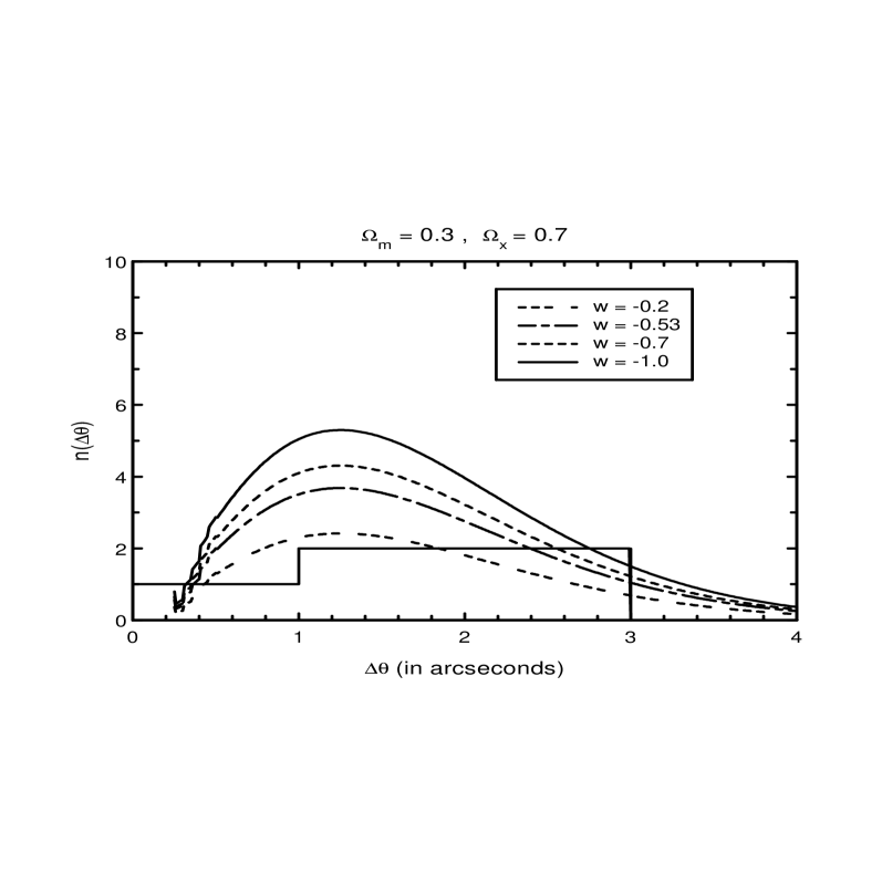
Figure 2: The expected distribution of lens image separations with $\Omega_{m}=0.3,\Omega_{x}=0.7$ compared with the observed image-separation distribution in the optical sample (histogram). The expected distribution is plotted for different values of $w$.

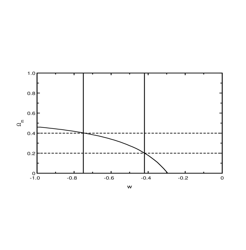
Figure 3: Contour between $\Omega_{m}$ and $w$ in order to get five lensed quasars in the optical sample. The dotted lines indicate the observed range of $\Omega_{m}\sim 0.2-0.4$. The vertical lines give the corresponding value of $w$.

References

- [1] S. Perlmutter et al., Nature, 391, 51 (1998).
- [2] S. Perlmutter et al., Astrophys. J., 517, 565 (1999).
- [3] A. Riess et al., Astron. J., 116, 1009 (1998).
- [4] P. M. Garnavich et al., Astrophys. J., 509, 74 (1998).
- [5] P. de Bernardis et al., Nature, 404, 955 (2000).
- [6] M. S. Turner, Physics Scripta, T85, 210 (2000).
- [7] V. Sahni and A. A. Starobinsky, Int. J. Mod. Phys. D, 9, 373 (2000).
- [8] M. Ozer & M.O. Taha, Nucl. Phys. B, 287, 776 (1987); I. Waga, Astrophys. J., 414, 436 (1993); L.F. Bloomfield Torres & I. Waga, Mon. Not. R. Astron. Soc., 279, 712 (1996); V. Silveria & I. Waga Phys. Rev. D, 56, 4625 (1997).
- [9] B. Ratra & P.J.E. Peebles, Phys. Rev. D , 37, 3406. (1988); J.A. Frieman et al., Phys. Rev. Lett., 75, 2077. (1995); J.A. Frieman & I. Waga, Phys. Rev. D , 57, 4642. (1998); R.R. Caldwell, R. Dave & P.J. Steinhardt, Phys. Rev. Lett., 80, 1582 (1998); I. Zlatev, L. Wang & P.J. Steinhardt, Phys. Rev. Lett., 82, 896 (1999); I. Waga & J.A. Frieman, Phys. Rev. D , 62, 043521 (2000).
- [10] D. Spergel & U.L. Pen, Astrophys. J., 491, L67 (1997).
- [11] M.S. Turner & M. White, Phys. Rev. D , 56, 4439. (1997); T. Chiba, N. Sugiyama & T. Nakamura, Mon. Not. R. Astron. Soc., 289, L5 (1997); D. Huterer & M.S. Turner, astro-ph/0012510 (2000).
- [12] I. Waga and A. P. M. R. Miceli Phys. Rev. D, 59, 103507. (1999)
- [13] J. A. S. Lima and J. S. Alcaniz, Mon. Not. R. Astron. Soc., 317, 893 (2000).
- [14] L.Wang et al., Astrophys. J., 530, 17 (2000).
- [15] Z. H. Zhu, Int. J. Mod. Phys. D, 9, 591 (2000).
- [16] P. Schechter, Astrophys. J., 203, 297 (1976).
- [17] C. S. Kochanek, Astrophys. J., 466, 47 (1996) [K96].
- [18] J. Loveday et al., Astrophys. J., 390, 38 (1992) [LPEM].
- [19] M. Fukugita et al., Astrophys. J., 393, 3 (1992).
- [20] C. S. Kochanek, Astrophys. J., 419, 12 (1993).
- [21] M. Chiba & Y. Yoshii, Astrophys. J., 510, 42 (1999).
- [22] A. R. Cooray and D. Huterer, Astrophys. J., 513, L95 (1999).
- [23] D. Christlein , Astrophys. J., 545, 145 (2000)
- [24] D. Jain, N. Panchapakesan, S. Mahajan and V. B. Bhatia, Mod. Phys. Lett. A, 15, 1 (2000).
- [25] A. Dekel, D. Burstein & S. White, in Critical Dialogues in Cosmology, edited by N. Turok (World Scientific, Singapore, 1997).
- [26] A. Balbi et al., Astrophys. J., 547, L89 (2001).
- [27] D. Jain, N. Panchapakesan, S. Mahajan and V. B. Bhatia, Int. J. Mod. Phys. A, 13, 4227 (1998).
- [28] R. Takahashi & T. Chiba, Preprint No. astro - ph/0106176 (2001)
- [29] D. Rusin & M. Tegmark, Preprint No. astro - ph/0008329 (2000)