Solar System Objects Observed in the Sloan Digital Sky Survey Commissioning Data¹

Abstract

We discuss measurements of the properties of $\sim$10,000 asteroids detected in 500 deg² of sky in the Sloan Digital Sky Survey (SDSS) commissioning data. The moving objects are detected in the magnitude range 14 $<$ $r^{*}$$<$ 21.5, with a baseline of $\sim$5 minutes, resulting in typical velocity errors of $\sim$3%. Extensive tests show that the sample is at least 98% complete, with the contamination rate of less than 3%.

We find that the size distribution of asteroids resembles a broken power-law, independent of the heliocentric distance: $D^{-2.3}$ for 0.4 km $\lesssim D\lesssim$ 5 km, and $D^{-4}$ for 5 km $\lesssim D\lesssim$ 40 km. As a consequence of this break, the number of asteroids with $r^{*}$$<$ 21.5 is ten times smaller than predicted by extrapolating the power-law relation observed for brighter asteroids ($r^{*}$$\lesssim$ 18). The observed counts imply that there are about 530,000 objects with $D>1$ km in the asteroid belt, or about four times less than previous estimates. We predict that by its completion SDSS will obtain about 100,000 near simultaneous five-band measurements for a subset drawn from 280,000 asteroids brighter than $r^{*}$$<$ 21.5 at opposition. Only about a third of these asteroids have been previously observed, and usually in just one band.

The distribution of main belt asteroids in the 4-dimensional SDSS color space is bimodal, and the two groups can be associated with S (rocky) and C (carbonaceous) asteroids. A strong bimodality is also seen in the heliocentric distribution of asteroids and suggests the existence of two distinct belts: the inner rocky belt, about 1 AU wide (FWHM) and centered at $R$ $\sim$2.8 AU, and the outer carbonaceous belt, about 0.5 AU wide and centered at $R$ $\sim$3.2 AU. The median color of each class becomes bluer by about 0.03 mag AU^-1 as the heliocentric distance increases. The observed number ratio of S and C asteroids in a sample with $r^{*}$$<$ 21.5 is 1.5:1, while in a sample limited by absolute magnitude it changes from 4:1 at 2 AU, to 1:3 at 3.5 AU. In a size-limited sample with $D>1$ km, the number ratio of S and C asteroids in the entire main belt is 1:2.3.

The colors of Hungarias, Mars crossers, and near-Earth objects, selected by their velocity vectors, are more similar to the C-type than to S-type asteroids, suggesting that they originate in the outer belt. In about 100 deg² of sky along the Celestial Equator observed twice two days apart, we find one plausible Kuiper Belt Object (KBO) candidate, in agreement with the expected KBO surface density. The colors of the KBO candidate are significantly redder than the asteroid colors, in agreement with colors of known KBOs. We explore the possibility that SDSS data can be used to search for very red, previously uncatalogued asteroids observed by 2MASS, by extracting objects without SDSS counterparts. We do not find evidence for a significant population of such objects; their contribution is no more than 10% of the asteroid population.

Submitted to AJ.

1 Introduction

The scientific relevance of the small bodies in our solar system ranges from fundamental questions about their origins to pragmatic societal concerns about the frequency of asteroid impacts on the Earth. A proper inventory of these objects requires a survey with

1. Large sky coverage.

2. Faint limiting magnitude.

3. Uniform and well-defined detection limits in magnitude and proper motion.

4. Accurate multicolor photometry for taxonomy.

5. Sufficient multi-epoch observations or follow-up observations to determine the orbits of all, or at least of particularly interesting objects.

The Sloan Digital Sky Survey (SDSS, York et al. 2000), which was primarily designed for studies of extragalactic objects, satisfies all of the above requirements, except the last one. Although the SDSS cannot be used to determine the orbits of detected moving objects (except in the special case of the Kuiper Belt Objects discussed in §8), its accurate and deep near simultaneous five-color photometry, ability to detect the motion of objects moving faster than $\sim$0.03 deg day^-1, and large sky coverage, can be efficiently used for studying small solar system objects. For example, the largest multi-color asteroid survey to date is the Eight Color Asteroid Survey (ECAS, Zellner, Tholen & Tedesco 1985), in which 589 asteroids were observed in eight different passbands. The five-color SDSS photometry spans roughly the same wavelength range as the ECAS passbands, and will be available for about 100,000 asteroids to a limit about seven magnitudes fainter than ECAS. This represents an increase in the number of observed objects with accurate multi-color photometry by more than two orders of magnitude. The only other survey with depth and number of observed objects comparable to SDSS is Spacewatch II (Scotti, Gehrels & Rabinowitz 1991), which, however, does not provide any color information. Color information is vital in e.g. determining the asteroid size distribution, which is considered to be the “planetary holy grail” by Jedicke & Metcalfe (1998), because the colors can be used to distinguish different types of asteroids and thus avoid significant ambiguities (Muiononen, Bowell & Lumme 1995). For informative reviews of asteroid research we refer the reader to Gehrels (1979) and Binzel (1989).

This paper presents some of the early solar system science from the SDSS commissioning data. These data cover about 5% of the total sky area to be observed by the survey completion (in about 5 years). Section 2 describes the SDSS, its capabilities for moving object detection, and the detection algorithm implemented in the photometric processing pipeline. The data and the accuracy of measured parameters are described in Section 3. The colors of detected objects are discussed in Section 4, and their proper motions in Section 5. The distributions of heliocentric distances and sizes of main belt asteroids are discussed in Section 6. We describe the use of SDSS data for finding asteroids in 2MASS data in Section 7, the search for Kuiper Belt Objects using multi-epoch SDSS data in Section 8, and discuss the results in Section 9.

2 Solar System Objects in SDSS

2.1 SDSS Imaging Data

The SDSS is a digital photometric and spectroscopic survey which will cover 10,000 deg² of the Celestial Sphere in the North Galactic cap and produce a smaller ($\sim$ 225 deg²) but much deeper survey in the Southern Galactic hemisphere (York et al. 2000 and references therein). The survey sky coverage will result in photometric measurements for about 50 million stars and a similar number of galaxies. The flux densities of detected objects are measured almost simultaneously in five bands ($u^{\prime}$, $g^{\prime}$, $r^{\prime}$, $i^{\prime}$, and $z^{\prime}$; Fukugita et al. (1996)) with effective wavelengths of 3561 Å, 4676 Å, 6176 Å, 7494 Å, and 8873 Å, 95% complete for point sources to limiting magnitudes of 22.1, 22.4, 22.1, 21.2, and 20.3 in the North Galactic cap. Astrometric positions are accurate to about 0.1 arcsec per coordinate (rms) for sources brighter than 20.5^m (Pier et al. 2001), and the morphological information from the images allows robust star-galaxy separation to $\sim$ 21.5^m (Lupton et al. 2001).

The SDSS footprint in ecliptic coordinates is shown in Figure 1. The survey avoids the Galactic plane, which is of limited use for solar system surveys anyway because of the dense stellar background. The survey is performed by scanning along great circles, indicated by solid lines. There are several important areas for solar system science. The obvious area is the coverage of the Ecliptic from $\lambda=100^{\circ}$ to $\lambda=225^{\circ}$. Less obvious is the area around $\lambda=100^{\circ}$ at one end of the great circle scans. Here, there will be significant convergence of the scans, so about half of the sky is scanned twice in the course of the survey. The third region, where the southern strip crosses the Ecliptic ($\lambda=0^{\circ}$), will be scanned several dozen times, and will be useful for studying the inclination and ecliptic latitude distributions of detected objects. The shaded regions represent areas analyzed in this work, and are described in more detail in Section 3.1.

2.2 The SDSS Sensitivity for Detecting Moving Objects

The SDSS camera (Gunn et al. 1998) detects objects in the order $r^{\prime}-i^{\prime}-u^{\prime}-z^{\prime}-g^{\prime}$, with detections in two successive bands separated in time by 72 seconds. The mean astrometric accuracy for band-to-band transformations is 0.040 arcsec per coordinate (Pier et al. 2001). With this accuracy, an $8\sigma$ moving object detection between the $r^{\prime}$ and $g^{\prime}$ bands corresponds to an angular motion of $\sim$0.025 deg/day (or 3.8 arcsec/hr). This limit corresponds to the Earth reflex motion for an object at a distance of $\sim$ 34 AU (i.e. the distance of Neptune) and shows that all types of asteroid (including Trojans) can be readily detected (assuming an object at opposition). With this level of accuracy it seems that the motion of Kuiper Belt Objects (KBOs), which are mostly found beyond Neptune’s orbit, could be detected at a significance level better than $\sim$6$\sigma$. Unfortunately, the distribution of the astrometric errors (which include contributions from centroiding and band-to-band transformations) is not strictly Gaussian, and the tests show that the KBOs would be effectively detected at only $\sim$3$\sigma$ level (a typical KBO would move about 0.3 arcsec between the $r^{\prime}$ and $g^{\prime}$ exposures). Since the stellar density at the faint magnitudes probed by SDSS is more than 10⁵ times larger than the expected KBO density ($\sim$ 0.05-0.1 deg^-2 for $r^{*}$$\lesssim$ 22, Jewitt 1999), the false candidates would preclude the routine detection of KBOs.

The upper limit on angular motion for detecting moving objects in a single scan with the present software is about 1 deg/day. This value is determined by the upper limit on the angular distance between detections of an object in two different bands, for them to be classified by the SDSS software as a single object. While somewhat seeing dependent (see the next section), it is sufficiently high not to impose any practical limitation for the detection of main belt asteroids.

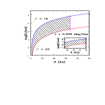
Figure 2: The SDSS sensitivity for finding moving objects in a single scan. The objects are assumed to be in circular orbits, have albedo of 0.1, and are observed at opposition. The upper limit on the object size is set by the image saturation, and the lower limit is set by the limiting magnitude for the survey ($r^{*}$$\sim$22). The upper limit on the heliocentric distance (or equivalently, the lower limit on the detectable motion) is set by the astrometric accuracy.

The SDSS coverage of the size – distance plane for objects on circular orbits observed close to the antisolar point is shown in Figure 2. The two curved lines represent the SDSS CCD saturation limit, $r^{*}$=14, and the faint limit $r^{*}$=22. They lines are determined from (e.g. Jewitt 1999)

$$\hbox{$r^{*}$}=\hbox{$r^{*}$}(1,0)+5\log[R(R-1)],$$ (1)

where the heliocentric distance, $R$, is measured in AU, and $\hbox{$r^{*}$}(1,0)$ is the “absolute magnitude”, the magnitude that an asteroid would have at a distance of 1 AU from the Sun and from the Earth, viewed at zero phase angle. This is an impossible configuration, of course, but the definition is motivated by desire to separate asteroid physical characteristics from the observing configuration. The absolute magnitude is given by

$$\hbox{$r^{*}$}(1,0)=17.9-2.5\log({p\over 0.1})-5\log(D/1{\rm km}),$$ (2)

where $p$ is the albedo, and the object diameter is $D$ (assuming a spherical asteroid). The constant 17.9 was derived by assuming that the apparent magnitude of the Sun in the $r^{\prime}$ band is -26.95, obtained from $V_{\odot}$ = -26.75 and $(B-V)_{\odot}=0.65$ (Allen 1973) with the aid of photometric transformations from Fukugita et al. (1996). This constant in an equivalent expression for the IAU-recommended (see e.g. Bowel et al. 1989) asteroid $H$ magnitude (not to be confused with the near-infrared $H$ magnitude at $\sim$1.65 $\mu{\rm m}$) is 18.1. The plotted curves can be shifted vertically by changing the albedo (we assumed $p=0.1$). The vertical line corresponds to an angular motion of 0.025 deg/day, approximately transformed into distance by using (e.g. Jewitt 1999)

$$v={0.986\over R+\sqrt{R}}\,\hbox{deg/day}.$$ (3)

The shaded region shows the part of the $D$–$R$ plane that can be explored with single SDSS scans. SDSS can detect main belt asteroids with radii larger than $\sim$ 100 m, while asteroids larger than $\sim$ 10-100 km, depending on their distance, saturate the detectors. The upper limit on the heliocentric distance at which motion can be detected in a single observation is $\sim$ 34 AU; at that distance SDSS can detect objects larger than 100 km (although the practical limit on heliocentric distance is somewhat smaller due to confusion with stationary objects, as argued above).

Without an improvement by about a factor of 2 in relative astrometry, single SDSS scans cannot be used to efficiently detect KBOs. However, multiple scans of the same area can be used to search for KBOs, and we describe such an effort in Section 8. The utilization of two-epoch data obtained on time scales of up to several days allows the detection of moving objects at distances as large as 100 AU. For example, at $R$ = 50 AU SDSS can detect objects larger than $\sim$ 200 km.

2.3 Detection of Moving Objects in SDSS Data

The SDSS photometric pipeline (Lupton et al. 2001) automatically flags all objects whose position offsets between the detected bands are consistent with motion. Without this special treatment, main belt and faster asteroids would be deblended into one very red and one very blue object, producing false candidates for objects with non-stellar colors. In particular, the candidate quasars selected for SDSS spectroscopic observations would be significantly contaminated because they are recognized by their non-stellar colors (Richards et al. 2001).

As discussed in the previous section, objects are detected in the order $r^{\prime}-i^{\prime}-u^{\prime}-z^{\prime}-g^{\prime}$, with detections in two successive bands separated in time by 72 seconds. The images of objects moving slower than about 0.5 deg/day (about 1 arcsec during the exposure in a single band) are indistinguishable from stellar; only extremely fast near-Earth objects are expected to be extended along the motion vector. After finding objects and measuring their peaks in each band, they are merged together by constructing the union of all pixels belonging to them. The five lists of peaks, one for each band, are then searched for peaks that appear at a given position (within 2$\sigma$) in only one band (if an object is detected at the same position in at least two bands it cannot be moving). When all the single-band peaks have been found, if there are detections in at least three bands, the algorithm fits for two components of proper motion; if the $\chi^{2}$ is acceptable ($<$3 per degree of freedom), and the resulting motion is sufficiently different from zero ($>2\sigma$), the object is declared moving.

For the traditional detection methods based on asteroid trails, the detection efficiency decreases with the speed of the asteroid at a given magnitude because the trail becomes fainter (e.g. Jedicke & Metcalfe, 1998). Any quantitative analysis needs to account for this effect, and the correction is difficult to determine. One of the advantages of SDSS is that the detection efficiency does not depend on the asteroid rate of motion within the relevant range (most asteroids move slower than 0.5 deg/day).

3 The Search for Moving Objects in SDSS Commissioning Data

3.1 The Selection of Moving Objects

We utilize a portion of SDSS imaging data from six commissioning runs (numbered 94, 125, 752, 756, 745, and 1336). The first four runs cover 481.6 deg² of sky along the Celestial Equator ($-1.27^{\circ}\lesssim{\rm Dec}\lesssim 1.27^{\circ}$) with the ecliptic latitude, $\beta$, ranging from -14^∘ to 20^∘, and the last run covers 16.2 deg² of sky with $73^{\circ}<\beta<86^{\circ}$. The fifth run (745) covers roughly the same sky region as run 756, and was obtained 1.99 days earlier. This two-epoch data set is used to determine the completeness of the asteroid sample and to search for KBOs. The data were taken during the Fall of 1998, the Spring of 1999, and the Spring of 2000. More details about these runs are given in Table 1. The data in each run were obtained in six parallel scanlines, each 13.5 arcmin wide (the six scanlines from adjacent runs are interleaved to make a filled stripe). The seeing in all runs was variable between 1 and 2 arcsec (FWHM) with the median values ranging from 1.3 to 1.7 arcsec.

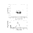
Figure 3: The upper panel shows the velocity distribution in equatorial coordinates for 11,216 moving object candidates (see text). The lower panel shows the velocity histogram for the same objects. Objects with $v<0.03\,\hbox{deg/day}$ are likely to be spurious.

We first select all point sources which are flagged as moving (see §2.3) and are brighter than $r^{*}$=21.5. We choose a more conservative flux limit that discussed above because the accuracy of the star-galaxy separation algorithm is not yet fully characterized at fainter levels (we note that repeated commissioning scans imply that significantly less than 5% of sources with $r^{*}$$\sim$21.5 are misclassified). There are 11,216 such moving object candidates in the analyzed area, and the upper panel in Figure 3 shows their velocity distribution in equatorial coordinates (for the four equatorial runs which dominate the sample, the $v_{RA}$ velocity component is parallel to the scanning direction). There are two obvious concentrations of objects whose velocities satisfy $v_{Dec}=\pm 0.43v_{RA}$. The angle between the velocity vector and the Celestial Equator is $\sim$ 23 deg (i.e. arctan(0.43)) because the velocity vector is primarily determined by the Earth reflex motion, and the asteroid density is maximal at the intersection of the Celestial Equator and the Ecliptic. There are two peaks because the sample includes both Spring and Fall data.

The candidates close to the origin ($v\lesssim 0.03$ deg/day, see the lower panel in Figure 3) are probably spurious detections since this velocity range is roughly the same as the expected sensitivity for detecting moving objects (see §2.2). Furthermore, we find that the distribution of these candidates is roughly circularly symmetric around the origin, which further reinforces the conclusion that they are not real detections. Consequently, in the remaining analysis we consider only the 10,678 moving object candidates with $v>0.03$ deg/day, which for simplicity we will call asteroids hereafter.

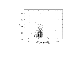
Figure 4: The $r^{*}$ vs. $v$ distribution for the 11,216 moving object candidates. The vertical strip of objects with $v\hbox{$\sim$}0$ are the rejected sources, and the large concentration of sources to the right are 10,678 selected asteroids. Note the strikingly empty gap between the two groups, which suggests that most detections with $v\gtrsim 0.03$ deg day^-1 are real.

The resulting sample is not very sensitive to the value of adopted cut, $v>0.03$ deg/day. Figure 4 shows the $r^{*}$ vs. $v$ distribution for the 11,216 moving object candidates. The vertical strip of objects with $v\hbox{$\sim$}0$ are the rejected sources, and the large concentration of sources to the right are 10,678 selected asteroids. Note the strikingly clean gap between the two groups indicating that the false moving object detections are probably well confined to a small velocity range. It is noteworthy that the objects with $v<0.03$ deg/day are not concentrated towards the faint end, i.e. they do not represent evidence that the moving object algorithm deteriorates for faint sources. The number of $\sim$ 500 objects appears consistent with the expected scatter due to the large number of processed objects ($\hbox{$\sim$}5\times 10^{6}$).

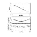
Figure 5: The top panel shows the positions in ecliptic coordinate system of 2757 asteroids, marked by dots, selected from run 752. The dash-dotted line shows the Celestial Equator. The bottom two panels show the longitude dependence of the two ecliptic components of the measured asteroid velocity (corrected for diurnal motion). The antisun is at $\lambda=180^{\circ}$. The curves show predictions for varying heliocentric distance and inclination (see text).

The SDSS scans are very long, and some asteroids are observed at large angles from the antisun direction. As discussed by Jedicke (1996), the observed velocity distribution is therefore significantly changed from the one that would be observed near opposition. Figure 5 shows the 2757 asteroids selected from run 752. The top panel displays each object as a dot in the ecliptic coordinate system. The overall scan boundaries, and to some extent the six column boundaries (the strip is made of six disjoint columns since the data from only one night are displayed), are outlined by the object distribution. Note that the density of objects decreases with the distance from the Ecliptic, as expected. The dash-dotted line shows the Celestial Equator. The lower two panels show the dependence of the two ecliptic components of the measured asteroid velocity, corrected for diurnal motion (i.e. the proper motion component due to the Earth’s rotation). These data were obtained on March 21, and thus the antisun is at $\lambda=180^{\circ}$. A strong correlation between the measured velocity and distance from the antisun, $\phi=\lambda-180^{\circ}$, is evident.

Following Jedicke (1996), we derive expressions for $v_{\lambda}(\phi,\beta,R,i)$ and $v_{\beta}(\phi,\beta,R,i)$ for a circular orbit (see Appendix A). The expected errors due to nonvanishing orbital eccentricity are 5-10%, depending on the heliocentric distance, $R$ and inclination, $i$ (e.g. Jedicke & Metcalfe 1998). The two lines in the upper part of the bottom panel show the predicted $v_{\lambda}(\phi)$ curves for $R$=2 AU (lower, solid) and $R$=3 AU (upper, dashed). The dependence of these curves on inclination is much smaller than on $R$ (the curves are computed for $i$ = 0^∘). Note that the curves cross for $|\phi|\hbox{$\sim$}40^{\circ}$. The two lines in the lower part of the bottom panel show the predicted $v_{\beta}(\phi)$ curves for $i$ = -10^∘ (lower, solid) and $i$ = 10^∘ (upper, dashed). The dependence of these curves on $R$ is much smaller than on inclination (the curves are computed for $R$=2.5 AU).

The plotted curves bracket the observed distribution, and show that it is impossible to accurately estimate the heliocentric distance for large $\phi$ since the $v_{\lambda}$ curves cross. Since the heliocentric distance is crucial for a significant part of the analysis presented here, we further limit the sample to $|\phi|<15^{\circ}$, except when studying the ecliptic latitude distribution (Section 4.2.1) and the dependence of colors on the phase angle (Section 6.2). This constraint produces a sample of 6666 asteroids. We estimate the heliocentric distance and orbital inclination for these asteroids as described in §3.4.2.

3.2 The Sample Completeness and Reliability

The sample completeness (the fraction of moving objects in the data recognized as such by the moving object algorithm) and reliability (the fraction of correctly recognized moving objects) are important factors which can significantly affect the conclusions derived in the subsequent analysis. It is not possible to determine the completeness and reliability by comparing the sample with catalogued asteroids because existing catalogs are complete only to $r^{*}$$\sim$15-16 (Zappala & Cellino 1996, Jedicke & Metcalfe 1998), while this sample extends to $r^{*}$= 21.5 (less than 1/3 of moving objects observed by SDSS can be linked to previously documented asteroids, see Appendix B). We estimate the sample completeness and reliability by analyzing data for 99.5 deg² of sky observed twice 1.9943 days apart (runs 745 and 756, see Table 1). These two runs were obtained during SDSS commissioning and overlap almost perfectly.

We estimate the sample reliability by matching 2474 objects selected by the moving object algorithm in run 756 to the source catalog for run 745. The probability that two moving objects would be found at an identical position in two runs is negligible, and such a matched pair indicates a stationary object that was erroneously flagged as moving. We find 62 matches within 1 arcsec implying a sample reliability of 97.5%. Visual inspection shows that the majority of false detections are either associated with saturated stars, or are close to the faint limit for detectability. Objects with very unusual velocities are more likely to be false detections; we discuss further the reliability of such candidates in Section 5.4.

The sample completeness can be obtained by comparing 2412 reliable detections to the “true” number of moving objects in the data. This “true” number can be estimated by using the fact that the true moving objects observed in one epoch will not have a positional counterpart in the other epoch. There are 4808 unsaturated point sources brighter than $r^{*}$=21.5 from run 756 that do not have counterparts within 3 arcsec in run 745 (the number of matched objects is $\hbox{$\sim$}10^{6}$). Not all 4808 unmatched objects are moving objects, as many are not matched due to instrumental effects (e.g. diffraction spikes, blended sources, etc.). The hard part is to select moving objects among these 4808 objects without relying on the moving object algorithm itself. We select the probable moving objects by using the difference between the point-spread-function (PSF) and “model” magnitudes in the $g^{\prime}$ band, and taking advantage of a bug in the code, since fixed.

The PSF magnitudes are measured by fitting a PSF model, and model magnitudes are measured by fitting an exponential and a de Vaucouleurs profile convolved with the PSF, and using the formally better model in the $r^{\prime}$ band to evaluate the magnitude (Lupton et al. 2001). Model magnitudes are designed for galaxy photometry and become equal to the PSF magnitudes for unresolved sources, if they are not moving. The difference between the PSF and model magnitudes for moving unresolved sources is due to different choices of centroids. For PSF magnitudes the local centroid in each band is used, while for model magnitudes the $r^{\prime}$ band center is used. The moving objects thus have fainter model magnitudes than PSF magnitudes in all bands but $r^{\prime}$ (the point sources have small $m_{psf}(\hbox{$r^{*}$})-m_{mod}(\hbox{$r^{*}$})$ by definition). This difference is maximized for the $g^{\prime}$ band and we find that 4808 unmatched sources show a bimodal distribution of $m_{psf}(\hbox{$g^{*}$})-m_{mod}(\hbox{$g^{*}$})$ with a well-defined minimum at about $-1$. There are 2424 sources with $m_{psf}(\hbox{$g^{*}$})-m_{mod}(\hbox{$g^{*}$})<-1$, and they can be considered as “true” moving objects (that is, we are essentially comparing two different detection algorithms). In the same area there are 2412 objects flagged by the moving object algorithm, and 2377 of these are included in the above 2424, implying that the sample completeness is 98% (this is indeed a lower limit on the sample completeness since it is possible that some of the 2424 sources with $m_{psf}(\hbox{$g^{*}$})-m_{mod}(\hbox{$g^{*}$})<-1$ are not truly moving).

3.3 The Accuracy of the Measured Velocities

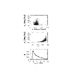
Figure 6: The velocity errors quoted by the moving object algorithm implemented in SDSS photometric pipeline. The top panel displays errors for 6,666 selected asteroids vs. the asteroid velocity magnitude, the middle panel shows errors vs. $r^{*}$ magnitude, and the bottom panel shows a histogram of fractional errors (expressed in percent).

While the sample completeness and reliability are sufficiently high for robust statistical analysis of the moving objects, inaccurate velocity measurements may contribute significant uncertainty because the heliocentric distance is determined from the asteroid rate of motion. Figure 6 gives an overview of the achieved accuracy, as quoted by the photometric pipeline. The top panel shows the velocity error vs. velocity, and the middle panel shows the velocity error vs. $r^{*}$ magnitude, where each of the 6666 asteroids is shown as a dot. It is evident that the errors are dominated by photon statistics at the faint end. The histogram of the fractional velocity errors displayed in the bottom panel shows that, for the majority of objects, the accuracy is better than 4%.

Of course, it is not certain whether the quoted errors are realistic. A test requires independent velocity measurements. We estimate the accuracy of the measured velocity by comparing two adjacent runs (752 and 756, see Table 1) obtained one day apart. These two runs can be interleaved to make a full stripe. Thanks to a fortuitous combination of the column width (13.5 arcmin) and the time delay between the two scans, many asteroids observed in the first run move into the area scanned by the second run the following night. Out of 1626 asteroids with $|\phi|<15^{\circ}$ observed in run 752, 693 were expected to be reobserved in run 756. For reobserved objects the velocity can be obtained about 300 times more accurately than from single run data, due to longer time baseline ($\sim$24 hours vs. $\sim$5 minutes).

We positionally match within 60 arcsec these 693 asteroids to the asteroids observed in run 756, and find 476 matches. By rematching a random set of positions within the same matching radius, we estimate that about 18 are random associations, implying a true matching rate of 66% (this matching rate is substantially lower than the reliability of the sample because of the velocity errors). The association of the two samples with a larger matching radius increases the number of close pairs but also increases the fraction of random associations. We find that matched and unmatched objects have similar magnitude distributions, showing that the algorithm is robust at the faint end.

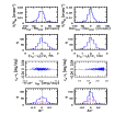
Figure 7: The comparison of asteroid velocities and quoted errors measured in a single observing run with the “true” values determined by reobserving objects the following night for 476 asteroids observed twice in runs 752 and 756. In the top two rows the left column corresponds to the right ascension component and the right column to the declination component. The top two panels show histograms of the positional difference, and the panels in the second row show the velocity difference normalized by the quoted error. The two panels in the third row show the velocity difference vs. the true velocity (left), and the velocity difference vs. the mean $r^{*}$ magnitude. The bottom two panels show the histograms of the magnitude and color differences between the two epochs for the asteroids observed twice. The solid lines show histograms for all objects, and the dot-dashed line show histograms for objects with $\hbox{$r^{*}$}<20$. Note that the magnitude difference histogram is significantly wider than the color difference histogram, presumably due to variability caused by the rotation of asteroids.

The detailed matching statistics are presented in Figure 7. The histograms of the differences between the predicted and observed positions in the second epoch are shown in the top row. As discussed earlier, the matched position can be used to determine the asteroid velocity to a much better precision than from single run data. The two panels in the second row in Figure 7 show the histograms of the difference between this “true” velocity and the measured velocity in run 756, normalized by the quoted errors. The quoted errors are overestimated by factor $\sim$2, presumably due to overestimated centroiding errors in the photometric pipeline (whose computation has been meanwhile improved). The two panels in the third row show that the velocity difference is correlated with neither the velocity nor the object’s brightness (if comparing these two panels with the middle panel in Figure 6, note that here only 476 matched objects are included, while there all 6666 objects are shown).

The same matched data can be used to test the photometric accuracy. The photometric errors determined by comparing measurements for stars observed in two epochs are about 2-3% for objects at the bright end, and then start increasing due to photon counting noise (for more details see Ivezić et al. 2000). The bottom two panels in Figure 7 show the histograms of the observed differences in $r^{*}$ magnitude (lower left panel) and asteroid $a^{*}$ color (to be defined in the next section, lower right panel). The histogram for all 476 matched asteroids is shown by a solid line, and for 165 asteroids with $\hbox{$r^{*}$}<20$ by a dot-dashed line. From the interquartile range we estimate that the equivalent Gaussian width of the $r^{*}$ histogram is 0.11 mag, and the width of the $a^{*}$ histogram is 0.07 mag, independent of the magnitude limit. The color histogram is narrower than the magnitude histogram, although its width is expected to be between 1 and $\sqrt{2}$ times wider than the width of the magnitude difference histogram, based on the statistical considerations. This may be interpreted as the variability due to asteroid rotation which affects the brightness but not the color. Such an interpretation was first advanced by Kuiper et al. (1958).

In the subsequent analysis we consider only the sample with 5253 unique sources, formed by excluding sources from runs 94 and 752 whose positions and velocities imply that they are also observed in runs 125 and 756, respectively. The uncertainty of measured velocities will result in some sources being incorrectly excluded, and some sources being counted twice. However, the excluded sources represent only $\hbox{$\sim$}24\%$ of the full sample, and thus even an uncertainty of 20% in the sample of excluded sources corresponds to less than 5% of the final sample. More importantly, no significant bias with respect to brightness, color, position, and velocity is expected in this procedure, as shown above.

4 The Asteroid Colors

4.1 The Colors of Main Belt Asteroids

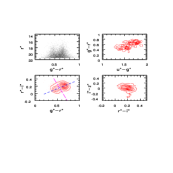
Figure 8: The color-magnitude and color-color diagrams for 5,125 main belt asteroids. The color-magnitude diagram in the upper left panel shows all objects as dots. The three color-color diagrams in other panels show the distributions of objects with photometric errors less than 0.05 mag. as linearly spaced isodensity contours, and as dots below the lowest level. Note the bimodal distribution in the $g^{*}-r^{*}$ vs. $u^{*}-g^{*}$ and $r^{*}-i^{*}$ vs. $g^{*}-r^{*}$ diagrams. The two dashed lines in the $r^{*}-i^{*}$ vs. $g^{*}-r^{*}$ diagram show a rotated coordinate system which defines an optimal asteroid color, named $a^{*}$.

The color-magnitude diagram for the 5,125 main belt asteroids (selected by their velocity vectors as described in §5.1 below) is displayed in the upper left panel in Figure 8. The other three panels display color-color diagrams. For clarity, in the last three diagrams the asteroid distribution is shown by linearly spaced density contours in the regions of high density and as dots outside the lowest level contour. It is evident that the asteroid color distribution is bimodal, in agreement with previous studies of smaller samples (Binzel 1989 and references therein). In particular, the two color types are clearly separated in the $r^{*}-i^{*}$ vs. $g^{*}-r^{*}$ color-color diagram which shows two well defined peaks.

The comparison of the observed color distributions with the colors of known asteroids observed in the SDSS bands by Krisciunas, Margon & Szkody (1998) shows that the “blue” asteroids in the $r^{*}-i^{*}$ vs. $g^{*}-r^{*}$ diagram (lower left peak) can be associated with the C type (carbonaceous) asteroids, while the redder class (upper right peak) corresponds to the S type (silicate, rocky) asteroids. However, note that not all “blue” asteroids are C type asteroids, and not all “red” asteroids are S type asteroids, but rather they contain other taxonomic classes as well. For example, Tedesco et al. (1989) defined 11 families among 357 asteroids, based on IRAS photometry and three wideband optical filters. The IRAS photometry is used to determine the albedo which, together with the two colors, defines the taxonomic classes. Nevertheless, the same work shows that a large majority of all asteroids belong to either C or S type, and we find that SDSS photometry clearly differentiates between the two types.

Tedesco et al. noted that much of the difference in the asteroid spectra between 0.3 $\mu{\rm m}$ and 1.1 $\mu{\rm m}$ is due to two strong absorption features, one bluer than 0.55 $\mu{\rm m}$ and one redder than 0.70 $\mu{\rm m}$. The SDSS $r^{\prime}$ filter lies almost entirely between these two absorption features, which may explain why the $\hbox{$g^{*}$}-\hbox{$r^{*}$}$ and $\hbox{$r^{*}$}-\hbox{$i^{*}$}$ colors provide good separation of the two color types. Moreover, the $r^{*}-i^{*}$ vs. $g^{*}-r^{*}$ color-color diagram is constructed with the most sensitive SDSS bands. We use this diagram to define an optimized color that can be used to quantify the correlations between asteroid colors and other properties (e.g. heliocentric distance, as discussed in the next section). We rotate and translate the $r^{*}-i^{*}$ vs. $g^{*}-r^{*}$ coordinate system such that the new x-axis, hereafter called $a^{*}$, passes through both peaks, and define its value for the minimum asteroid density between the peaks to be 0 (i.e. we find the principal components in the $r^{*}-i^{*}$ vs. $g^{*}-r^{*}$ color-color diagram). We obtain

$$\hbox{$a^{*}$}=0.89(\hbox{$g^{*}$}-\hbox{$r^{*}$})+0.45(\hbox{$r^{*}$}-\hbox{$i^{*}$})-0.57.$$ (4)

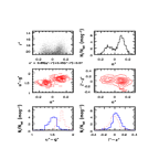
Figure 9: The $a^{*}$ color based color-magnitude and color-color diagrams and various histograms for 5,125 main belt asteroids. The bottom panels show color histograms for the two classes of asteroids, separated by their $a^{*}$ color ($a^{*}<0$, thick solid line; $a^{*}\geq 0$, thin dashed line).

Asteroids with $a^{*}$$<$ 0 are blue in the $r^{*}-i^{*}$ vs. $g^{*}-r^{*}$ diagram, and those with $a^{*}$$>$ 0 are red. Figure 9 shows various diagrams constructed with this optimized color. The top left panel displays the $r^{*}$ vs. $a^{*}$ color-magnitude diagram. The two color types are much more clearly separated than in the analogous diagram using the $g^{*}-r^{*}$ color (displayed in the top left panel in Figure 8). The top right panel shows the $a^{*}$-histogram for asteroids brighter than $r^{*}$=20. The number of main belt asteroids with $\hbox{$a^{*}$}>0$ is 1.88 times larger than the number of asteroids with $a<0$ (1.47 times for $r^{*}$$<$ 21.5). However, note that this result does not represent a true number ratio of the two types because the same flux limit does not correspond to the same size limit due to different albedos, and because of their different radial distributions (see Section 6).

The two middle panels show the color-color diagrams constructed with the new color. These diagrams suggest that the distribution of the SDSS colors for the main belt asteroids reveals only two major classes: the asteroids with $a^{*}$$<$ 0 have bluer $u^{*}-g^{*}$ color and slightly redder $i^{*}-z^{*}$ color than asteroids with $a^{*}$$>$ 0. These color differences are better seen in the color histograms shown in the two bottom panels, where thick solid lines correspond to asteroids with $a^{*}\leq 0$, and the thin dashed lines to those with $a^{*}>0$. In the remainder of this work we will refer to “blue” and “red” asteroids as determined by their $a^{*}$ color, but note that the $i^{*}-z^{*}$ colors are reversed (the subsample with bluer $i^{*}-z^{*}$ color is redder in other SDSS colors).

4.1.1 Does SDSS Photometry Differentiate More Than Two Color Types?

The large number of detected objects and accurate 5-color SDSS photometry may allow for a more detailed asteroid classification. For example, some objects have very blue $i^{*}-z^{*}$ colors ($<-0.2$, see Figure 9) which could indicate a separate family. There are various ways to form self-similar classes, well described by Tholen & Barucci (1989). We decided to use the program AutoClass in an unsupervised search for possible structure. AutoClass employs Bayesian probability analysis to automatically separate a given data base into classes (Goebel et al. 1989). This program was used by Ivezić & Elitzur (2000) to demonstrate that the IRAS PSC sources belong to four distinct classes that occupy separate regions in the 4-dimensional space spanned by IRAS fluxes, and the problem at hand is mathematically equivalent.

AutoClass separated main-belt asteroids into 4 classes by using 5 SDSS magnitudes (not the colors!) for objects brighter than $r^{*}$=20. The largest 2 classes include more than 98% of objects and are easily recognized in color-color diagrams as the two groups discussed earlier. The remaining 2% of sources are equally split in two groups. One of them is the already suspected group with $\hbox{$i^{*}-z^{*}$}<-0.2$. The inspection of color-color diagrams for these sources shows that the blue $i^{*}-z^{*}$ color is their only clearly distinctive characteristic. The remaining group is similar to the “blue” group but has $\sim$0.2 mag. redder $i^{*}-z^{*}$ color and $\sim$0.1 mag. bluer $r^{*}-i^{*}$ color. Since the number of asteroids in the two additional groups proposed by AutoClass is only 2%, we retain the original manual classification into two major types in the rest of this work.

4.1.2 Comparison With Independent Taxonomic Classification

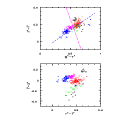
Figure 10: The synthetic color-color diagrams for the 316 asteroids whose spectra were obtained by the SMASS Survey, and convolved with the SDSS response functions (see text). The taxonomic class is shown by different symbols: crosses for the C type, dots for S, circles for D, solid squares for A, open squares for V, solid triangles for J, and open triangles for the E, M and P types (which are indistinguishable by their colors). The dashed lines in the upper panel show the principal axes from Figure 8.

The number of known asteroids observed through SDSS filters (Krisciunas, Margon & Szkody 1998) is too small for a robust statistical analysis of the correlation between the taxonomic classes and their color distribution. In order to investigate whether the known asteroids with independent taxonomic classification (which also includes the albedo information, not only the colors) segregate in the SDSS color-color diagrams, we synthesize their colors from spectra obtained by Xu et al. (1995). Their Small Main-belt Asteroid Spectroscopic Survey (SMASS) includes spectra for 316 asteroids with wavelength coverage from 0.4 $\mu{\rm m}$ to 1.0 $\mu{\rm m}$, with the resolution of the order 10 Å. We convolved their spectra with the SDSS response functions for the $g^{\prime},r^{\prime},i^{\prime},$ and $z^{\prime}$ bands (the spectra do not extend to sufficiently short wavelengths for synthesizing the $u^{\prime}$ band flux). The results are summarized in the color-color diagrams displayed in Figure 10. The taxonomic classification (also adopted from Xu et al.) is shown by different symbols: crosses for the C type, dots for S, circles for D, solid squares for A, open squares for V, solid triangles for J, and open triangles for the E, M and P types (which are indistinguishable by their colors). The dashed lines in the upper panel show the principal axes discussed above.

These diagrams show that the blue asteroids ($a^{*}<0$) include the C, E, M and P classes, while the red asteroids ($a^{*}\geq 0$) include the S, D, A, V, and J classes. Their distribution in the $r^{*}-i^{*}$ vs. $g^{*}-r^{*}$ diagram seems to be consistent with the bimodal distribution reported here. The segregation of the classes in the $i^{*}-z^{*}$ vs. $r^{*}-i^{*}$ diagram is evident. It may be that the D class asteroids could be separated by their red $i^{*}-z^{*}$ color ($>0.15$), and that the V and J classes could be separated by their blue $i^{*}-z^{*}$ color ($<-0.2$). However, note that the number of sources in these classes shown in Figure 10 is not representative of the SDSS sample due to a different selection procedure employed by the SMASS. Restricting the analysis to asteroids with $r^{*}$$<$20, we find that $\sim$6% of the sample have $\hbox{$i^{*}-z^{*}$}<-0.2$, and another 6% have $\hbox{$i^{*}-z^{*}$}>0.15$ (these fractions are somewhat higher than obtained by AutoClass because its Bayesian algorithm is intrinsically biased against overclassification, Goebel et al. 1989). We leave further analysis of such classification possibilities for future work, and conclude that the synthetic colors based on the SMASS data agree well with the observed color distribution.

4.1.3 Albedos

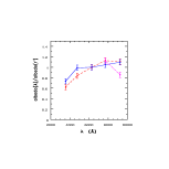
Figure 11: The mean albedo for the two color types of main belt asteroids normalized to its $r^{*}$-band value. The solid line is for 1841 asteroids with $a^{*}<0$, and the dashed line is for 3302 asteroids with $a^{*}\geq 0$. The mean albedo for a subset of the former, selected by $i^{*}-z^{*}$$<$ -0.20, is shown by the dot-dashed line. The error bars show the distribution width for each subsample (equivalent Gaussian width) – they are not errors of each point, whose uncertainty is smaller than the symbol size.

The observed differences in the color distributions reflect differences in asteroid albedos. Although the SDSS photometry cannot be used to estimate the absolute albedos (which would require the measurements of the thermal emission, see e.g. Tedesco et al. 1989), the spectral shape of the albedo can be easily calculated since the colors of the illuminating source are well known ($(\hbox{$u^{*}-g^{*}$})_{\odot}$ = 1.32, $(\hbox{$g^{*}-r^{*}$})_{\odot}$ = 0.45, $(\hbox{$r^{*}-i^{*}$})_{\odot}$ = 0.10, $(\hbox{$i^{*}-z^{*}$})_{\odot}$ = 0.04). Figure 11 shows the albedos obtained for the median color for the two color-selected types normalized to the $r^{\prime}$-band value. The error bars show the (equivalent Gaussian) distribution width for each subsample. The solid curve corresponds to asteroids with $\hbox{$a^{*}$}\geq 0$, and the dashed curve to those with $\hbox{$a^{*}$}<0$. Note the local maximum for the $\hbox{$a^{*}$}\geq 0$ type, and that the $u^{*}-g^{*}$ and $\hbox{$r^{*}$}-\hbox{$z^{*}$}$ colors are almost identical for the two types. The dotted curve shows the mean albedo for asteroids selected from the $\hbox{$a^{*}$}\geq 0$ group by requiring $i^{*}-z^{*}$$<-0.2$. The displayed wavelength dependence of the albedo is in good agreement with available spectroscopic data (e.g. compare to Figure 5 in Tholen & Barucci 1989, see also Figure 2 in Xu et al. 1995).

The subsequent analysis of the asteroid size distribution requires the knowledge of the absolute albedo for each color type. The typical absolute values of albedos for the two major asteroid types can be estimated from data presented by Zellner (1979). Following Shoemaker et al. (1979), we adopt 0.04 (in the $r^{\prime}$ band) for the C-like asteroids ($a^{*}<0$) and 0.14 for the S-like asteroids ($a^{*}\geq 0$). The intrinsic spread of albedo for each class is of the order 20%, in agreement with the range obtained by using IRAS data (Tedesco et al. 1989). This difference in albedos implies that a C-like asteroid is $\sim$1.4 magnitudes fainter than an S-like asteroid of the same size and at the same observed position, and that a C-like asteroid with the same apparent magnitude and observed at the same position is twice as large as an S-like asteroid.

4.2 The Asteroid Counts vs. Color

4.2.1 The Ecliptic Latitude Distribution

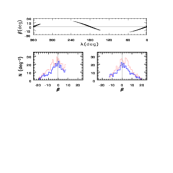
Figure 12: The ecliptic latitude distribution for 10,678 asteroids with $r^{*}$$<$ 21.5. The top panel shows the observed angular (sky) distribution. The two bottom panels show the dependence of the observed surface density on ecliptic latitude for the Fall (left, $\lambda\hbox{$\sim$}0^{\circ}$) and Spring (right, $\lambda\hbox{$\sim$}180^{\circ}$) samples. The two curves in each panel correspond to asteroids with $a^{*}<0$ (thick line) and with $a^{*}>0$ (thin line).

Figure 12 shows the dependence of the observed asteroid surface (sky) density on ecliptic latitude. The top panel shows the distribution of the 10,678 asteroids with $r^{*}$$<$ 21.5 in the ecliptic coordinate system, where each object is shown as a dot. The bottom two panels show the surface density vs. ecliptic latitude where the thick lines correspond to $a^{*}<0$ and thin lines to $a^{*}>0$. The bottom left panel shows the results for the Fall sample ($\lambda\hbox{$\sim$}0^{\circ}$) and the bottom right panel shows the results for the Spring sample $\lambda\hbox{$\sim$}180^{\circ}$).

It is evident that the ecliptic latitude distribution of the main belt asteroids is not very dependent on their color. The distribution of the Spring sample is centered on $\beta\hbox{$\sim$}2.0^{\circ}$, and the distribution of the Fall sample is centered on $\beta=-2.0^{\circ}$, in agreement with the distribution of catalogued asteroids (see Appendix B). The density of asteroids decreases rapidly with increasing ecliptic latitude and drops to below 1 deg^-2 for $\beta>20^{\circ}$. We do not detect a single moving object in 16.2 deg² of sky with $\beta\hbox{$\sim$}$80^∘ (run 1336, see Table 1).

The highest density of objects brighter than $r^{*}=21.5$ is $46\pm 2$ deg^-2 (including both color types). The mean density integrated over ecliptic latitudes is 780 asteroids per degree of the ecliptic longitude (determined by counting observed asteroids and accounting for all incompleteness effects). Assuming that this result is applicable to the entire asteroid belt (the observed numbers of asteroids agree to within 1% between the Fall and Spring subsamples), we estimate that there are $\sim$280,000 asteroids brighter than $r^{*}=21.5$ (observed near opposition). This estimate implies that SDSS will observe $\hbox{$\sim$}100,000$ asteroids by its completion (see Figure 1). We note that a fraction of these observations may be measurements of the same asteroids. This fraction depends on the details of which areas of sky are observed when, and cannot be estimated beforehand.

4.2.2 The Apparent Magnitude Distribution

The brightness distribution of asteroids can be directly transformed into their size distribution if all asteroids have the same albedo, and either have the same heliocentric distance, or the size distribution is a scaleless power law. While none of these conditions is true, we discuss the counts of asteroids as a function of apparent magnitude because they clearly differ for the two color types. The relationship between the distribution of apparent magnitudes and heliocentric and size distributions is discussed in more detail in Section 6 below.

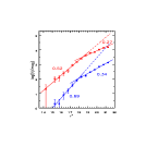
Figure 13: The differential counts for the two types of main-belt asteroids separated by their $a^{*}$ color. The open squares correspond to asteroids with $a^{*}>0$ and the large dots to asteroids with $a^{*}<0$. The former are shifted up by a factor of 10 for clarity. The error bars are computed by assuming Poisson statistics. The lines show the best fit broken power laws. The numbers show the best fit power-law indices for each magnitude range; other parameters are listed in Table 3.

The measured counts for main-belt asteroids, separated by their $a^{*}$ color, are shown in Figure 13 (here we do not apply the phase angle correction, see Section 6.1). The circles correspond to asteroids with $\hbox{$a^{*}$}<0$, and the squares correspond to the $\hbox{$a^{*}$}>0$ asteroids. The latter are shifted upwards by 1 dex for clarity. A striking feature visible in both curves is the sharp change of slope around $r^{*}$$\sim$18-19. We find that for both color types the counts vs. magnitude relation can be described by a broken power law

$$\log(N)\propto C_{B}+k_{B}\hbox{$r^{*}$}$$ (5)

for $r^{*}$$<r^{*}_{b}$, and

$$\log(N)\propto C_{F}+k_{F}\hbox{$r^{*}$}$$ (6)

for $r^{*}$$>r^{*}_{b}$, where $r^{*}_{b}$ is the magnitude for the power law break. The best fits are shown by lines in Figure 13, and the corresponding parameters are listed in Table 3.

The changes in the slope of the counts vs. magnitude relations could be caused by systematic effects in the detection algorithm. The dashed lines in Figure 13 show the extrapolation of the bright end power-law fit, and indicate that a decrease of detection efficiency by a factor of $\sim$10 is required to explain the observed counts at $r^{*}$$\sim$21.5. However, such a significant decrease of detection efficiency is securely ruled out (see Section 3.2). In summary, the number of asteroids with $r^{*}$$\sim$21 is roughly ten times smaller than would expected from extrapolation of the power-law relation observed for $r^{*}$$\lesssim$ 18.

The changes in the slope of the counts vs. magnitude relations disagree with a simple model proposed by Dohnanyi (1969), which is based on an equilibrium cascade in self-similar collisions, and which predicts a universal slope of 0.5. We will discuss this discrepancy further in Sections 6 and 9.

5 The Ecliptic Velocity and Determination of the Heliocentric Distance

5.1 The Velocity-Based Classification of Asteroids

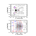
Figure 14: The velocity distribution in ecliptic coordinates for the 5,253 reliably detected moving objects. The lines in the top panel show the adopted separation of the objects into main belt asteroids, Trojans, Centaurs, Hungarias, Hildas, Mars crossers, near Earth objects (NEO), and Unknown. The lines in the bottom panel show the predictions for varying heliocentric distance ($R$) and inclinations ($i$), as marked (see text for details).

Figure 14 shows the velocity distribution in ecliptic coordinates for the sample of 5,253 unique asteroids. Its overall morphology is in agreement with other studies (e.g. Scotti, Gehrels & Rabinowitz 1991, Jedicke 1996) and shows a large concentration of the main belt asteroids at $v_{\lambda}\hbox{$\sim$}$ -0.22 deg/day and $v_{\beta}\hbox{$\sim$}0$. The sharp cutoff in their distribution at $v_{\lambda}\hbox{$\sim$}$ -0.28 deg/day is not a selection effect and corresponds to objects at a heliocentric distance of $\sim$ 2 AU. The lines in the top panel of Figure 14 show the boundaries adopted in this work for separating asteroids into different families, including the main belt asteroids, Hildas, Hungarias and Mars crossers, Trojans, Centaurs, as well as near Earth objects (NEOs). This separation in essence reflects different inclinations and orbital sizes of various asteroid families (for more details see e.g. Gradie, Chapman & Williams 1979, Zellner, Thirunagari & Bender 1985). These regions are modeled after the Spacewatch boundary for distinguishing NEOs from other asteroids (Rabinowitz 1991), information provided in Jedicke (1996), and taking into account the velocity distribution observed by SDSS.

There is some degree of arbitrariness in the proposed boundaries, for example the regions corresponding to Hungarias and Mars crossers could be merged together. The boundary definitions and asteroid counts for each region are listed in Table 2 (as indicated in the table, the visual inspection shows that some objects are spurious; see §5.4 below). These subsamples are used for comparative analysis of their colors and spatial distributions in the following sections. We emphasize that this separation cannot be used as a definitive identification of an asteroid with a particular family. In particular, the main belt asteroids may cause significant contamination of other regions due to the measurement scatter and their large number compared to other families.

5.2 The Correspondence between the Velocity and Orbital Elements

Six orbital elements are required to define the motion of an asteroid. Since the SDSS observations determine only four parameters (two sky coordinates and two velocity components) the orbit is not fully constrained by the available data. There are various methods to obtain approximate estimates for the orbital parameters from the asteroid motion vectors (e.g. Bowell, Skiff, Wasserman & Russell 1989, and references therein). These methods provide an accuracy of about 0.05-0.1 AU for determining the semimajor axes, and 1-5 deg. for the inclination accuracy. As shown by Jedicke & Metcalfe (1998), similar accuracy can be obtained by assuming that the orbits are circular.

We follow Jedicke (1996) and derive the expressions for observed ecliptic velocity components in terms of $R$, $i$ and $\phi$ listed in Appendix A. We show in Appendix B that these expressions can be used to estimate the heliocentric distance at the time of observation with an accuracy of 0.28 AU (rms). The uncertainty in the estimated heliocentric distance is significantly larger than the uncertainty in the estimated semimajor axes (0.07 AU) because asteroid orbits in fact have considerable eccentricity ($\sim$0.10-0.15). However, we emphasize that the estimates for heliocentric distance and semimajor axes are simply proportional to each other (for more details see Appendix B). The uncertainty of 0.28 AU in the estimate of heliocentric distance contributes an uncertainty of 0.5-0.8 mag. in the absolute magnitude (see eq. 1).

The bottom panel in Figure 14 magnifies the part of the top panel which includes the main belt and Hilda asteroids. The dashed lines show the loci of points with $i$ ranging from $-15^{\circ}$ to $15^{\circ}$ in steps of $5^{\circ}$, and the solid lines show loci of points with $R$ = 2, 2.5, 3 and 3.5 AU (the inclination is a positive quantity by definition; here we use negative values as a convenient way to account for different orbital orientations). They are computed by using eqs. Solar System Objects Observed in the Sloan Digital Sky Survey Commissioning Data¹ and Solar System Objects Observed in the Sloan Digital Sky Survey Commissioning Data¹ listed in Appendix A with $\beta=0$ and $\phi=0$. By using equations $2-6$ with the proper $\beta$ and $\phi$, we compute $R$ and $i$ for all 5,125 main belt asteroids in our sample.

5.3 The Relation between Color and Heliocentric Distance

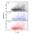
Figure 15: The distribution of 5,125 main belt asteroids in the sin($i$) vs. $R$ plane. The top panel shows the whole sample, while the other two panels show each color type separately, as marked. Note that the red asteroids (bottom panel) tend to have smaller heliocentric distances than do the blue asteroids (middle panel).

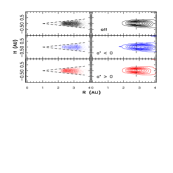
Figure 16: The cross section of the asteroid belt. In the left column each asteroid is shown as a dot, and in the right column the distribution is outlined by isodensity contours. The top panels show the whole sample, and the other panels show each color type separately, as marked. The two dashed lines in the left column are drawn at $\beta=\pm 8^{\circ}$ and show the observational limits. The vertical dashed lines in the right column show the position of the highest asteroid density for the red subsample and are added to guide the eye. Note that the distributions of blue and red asteroids are significantly different.

The $i-R$ distribution of the 5,125 main belt asteroids is shown in the top panel in Figure 15. The overall morphology is in agreement with other studies (e.g. see figure 1 of Zappala et al. 1990). The multi-color SDSS data allow the separation of asteroids into two types, and the middle and bottom panels show the distribution of each color type separately. Because the heliocentric distance estimates have an accuracy of 0.28 AU, these data cannot resolve narrow features. Nevertheless, it is evident that the red asteroids tend to be closer to the Sun. Another illustration of the differences in the distribution of the two color types is shown in Figure 16 which displays the cross-section of the asteroid belt: the horizontal axis is the heliocentric distance and the vertical axis is the distance from the ecliptic plane. The top panel shows the distribution of all asteroids and the middle and bottom panels show the distribution of each color type separately. The dashed lines in the left column are drawn at $\beta=\pm 8^{\circ}$  and show the observational limits. The dashed lines in the right column mark the position of the maximum density and are added to guide the eye. Note that the maximum density for blue asteroids (middle panel) lies about 0.4 AU further out than for red asteroids.

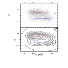
Figure 17: The color–heliocentric distance dependence in asteroid belt. In the top panel each asteroid is shown as a dot, and in the bottom panel the distribution is outlined by isodensity contours. Two dashed lines are fitted separately for $a^{*}<0$ and $a^{*}\geq 0$ subsamples. Note that each subsample tends to become slightly bluer as the heliocentric distance increases.

If the mean color varies strongly with heliocentric distance, splitting the sample by color would split the sample by heliocentric distance as well, explaining the shifting maxima in Figure 16. However, the dependence of color on the heliocentric distance shown in Figure 17 indicates that this is not the case. In the top panel each asteroid is marked as a dot, and the bottom panel shows the isodensity contours. It is evident that the bimodal color distribution persists at all heliocentric distances. The distributions of both types have a well defined maximum, evident in the bottom panel, which may be interpreted as the existence of two distinct belts: the inner, relatively wide belt dominated by red (S-like) asteroids and the outer, relatively narrow belt, dominated by blue (C-like) asteroids. We emphasize that the detailed radial distribution of asteroids in this diagram is strongly biased by the heliocentric distance dependent faint limit in absolute magnitude, and these effects will be discussed in more quantitative detail in Section 6. Nevertheless, the difference between the two types is not strongly affected by this effect, and the remarkable split of the asteroid belt into two components is a robust result.

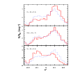
Figure 18: The color distributions for three main belt asteroid subsamples selected by their heliocentric distance, as indicated in the panels. Each panel compares the color distribution of a given subsample, shown as the solid line, to the color distribution of all main belt asteroids, shown as the dashed line.

Another notable feature displayed by the data is that the median color for each type becomes bluer with the heliocentric distance. The dashed lines in Figure 17 are linear fits to the color-distance dependence, fitted for each color type separately. The best fit slopes are (0.016$\pm$0.005) mag AU^-1 and (0.032$\pm$0.005) mag/AU for blue and red types, respectively. Due to this effect, as well as to the varying number ratio of the asteroid types, the color distribution of asteroids depends strongly on heliocentric distance. Figure 18 compares the $a^{*}$-color histograms for three subsamples selected by heliocentric distance: $2<R<2.5,2.5<R<3$, and $3<R<3.5$. The thick solid lines show the color distribution of each subsample, and the thin dashed lines show the color distribution of the whole sample.

5.4 The Reliability of Asteroids with Unusual Velocities

While the sample reliability is estimated to be 98.5% in Section 3.2, it is probable that it is much lower for asteroids with unusual velocities. To estimate the fraction of reliable detections for such asteroids, we visually inspect images for the 128 asteroids which are not classified as main belt asteroids. As a control sample, and also for an additional reliability estimate, we inspect 50 randomly selected main belt asteroids, and the 50 brightest and 50 faintest main belt asteroids. While the visual inspection of 278 images for the motion signature may seem a formidable task, it is indeed quite simple and robust. Since asteroids move they can be easily recognized by their peculiar colors in the $g^{\prime}-r^{\prime}-i^{\prime}$ color composites. Moving objects appear as aligned green–red–blue “stars”, with the blue-red distance three times larger than the green-red distance (due to filter spacings, see Section 2.3).

We find that neither of the two candidates for Centaurs are real. About 63% of NEOs (12/19), 57% of Mars crossers (4/7), 50% of Trojans (1/2) and 43% of Unknown (6/14) are not real. The contamination of the remaining subsamples is lower; only 5% for Hildas (3/59), while all 25 Hungarias are real. The majority of false detections are either associated with saturated stars, or are close to the faint limit. For all 3 subsamples with main belt asteroids the contamination is 2% (there is 1 instrumental effect per 50 objects in each class). Since the fraction of objects not classified as main belt asteroids is very small ($\sim$2%), these results are consistent with estimates described in §3.2.

5.5 The Colors of Asteroid Families Other than Main Belt

The color distributions of various families are particularly useful for linking them to other asteroid populations and constraining theories for their origin. For example, one possible source of the NEOs is the main belt asteroids near the 3:1 mean motion resonance with Jupiter. These asteroids have chaotic orbits whose eccentricities increase until they become Mars crossing, after which they are scattered into the inner solar system (Wisdom 1986). If this scenario is true, the colors of both the NEOs and Mars crossers should resemble the colors of main belt asteroids, but show more similarity to the C-type asteroids than to the whole sample due to the radial color gradient. An alternative source of NEOs is extinct comet nuclei; this hypothesis predicts a wider color range than observed for asteroids. Yet another hypothesis was forwarded by Bell et al. (1989) who predicted that NEOs should be more similar to S type than to C type asteroids. While there seems to be more evidence supporting the first hypothesis (Shoemaker et al. 1979), the analyzed samples are small.

We find that $\sim$70% of the visually confirmed NEOs (5/7), Unknown (6/8) Hungarias (17/25), and Mars crossers (2/3) belong to the blue type ($a^{*}<0$). More than half of the remaining 30% are typically borderline red ($a^{*}<0.05$). This is in sharp contrast with the overall color distribution of main belt asteroids, where the fraction of blue asteroids is only $\sim$40%, and the fraction of asteroids with $a^{*}<0.05$ is $\sim$47%. The result for NEOs implies that their source is the asteroid belt, rather than extinct comet nuclei. Furthermore, it supports the hypothesis they originate in the outer part of the asteroid belt, contrary to the prediction by Bell et al.. The colors of Hungarias and NEOs are similar, which is in agreement with the notion that Hungarias are an intermediate phase for the main belt asteroids on their route to becoming the NEOs. While it is not clear what the origin of asteroids from the “Unknown” region is, they are as blue as are Hungarias and NEOs.

The only confirmed Trojan candidate is distinctively red ($a^{*}=0.29$). Such a red color seems to agree with the colors of some Centaurs (Luu & Jewitt 1996) though it is hard to judge the significance of this result. We note that the Kuiper Belt object candidate discussed in Section 8 is also significantly redder ($a^{*}\hbox{$\sim$}0.6$) than the main belt color distribution.

6 The Heliocentric Distance and Size Distributions

The size distribution of asteroids is one of most significant observational constraints on their history (e.g. Jedicke & Metcalfe 1998, and references therein). It is also one of the hardest quantities to determine observationally because of strong selection effects. Not only that the smallest observable asteroid size in a flux limited sample strongly varies with the heliocentric distance, but the conversion from the observed magnitude to asteroid size depends on the, usually unknown, albedo. Assuming a mean albedo for all asteroids may lead to significant biases since the mean albedo depends on the heliocentric distance due to varying chemical composition. Because of its multi-color photometry, SDSS provides an opportunity to disentangle these effects by separately treating each of the two dominant classes, which are known to have rather narrow albedo distributions (see Section 4.1.2).

For a fixed albedo, the slope of the counts vs. magnitude relation, $k$, is related to the power-law index, $\alpha$, of the asteroid differential size distribution, $dN/dD=n(D)\propto D^{-\alpha}$, via

$$k=0.2(\alpha-1).$$ (7)

This simple relation assumes that the size distribution is a scale-free power law independent of distance, which results in a linear relationship between log(counts) and apparent magnitude. However, the observed change of slope around $r^{*}$$\sim$18 in the differential counts of asteroids (discussed in Section 4.2.3) introduces a magnitude scale which prevents a straightforward transformation from the counts to size distribution.

In the limit where a single power law is a good approximation to the observed counts, the above relation can still be used and shows that the power law index $\alpha$ of the asteroid size distribution is $\sim$4 at the bright end and $\sim$2.5 at the faint end for both color families (see Table 3). Since these values may be somewhat biased by the phase angle effect, and the strong dependence of the faint cutoff for absolute magnitude on heliocentric distance, in this section we perform a detailed analysis of the observed counts. By applying techniques developed for determining the luminosity function of extragalactic sources, we estimate unbiased size and heliocentric distance distributions for the two asteroid types.

6.1 The Correction for the Phase Angle

The observed apparent magnitude of an asteroid strongly depends on the phase angle, $\gamma$, the angle between the Sun and the Earth as viewed from the asteroid

$$\gamma={\rm arcsin}\left({\sin(\phi)\over R}\right).$$ (8)

We first determine the “uncorrected” absolute magnitude from

$$\hbox{$r^{*}$}(1,0)=\hbox{$r^{*}$}-5\log(R\rho),$$ (9)

where $\rho$ is the Earth-asteroid distance expressed in AU,

$$\rho=-\cos(\phi)+\left(\cos(\phi)+R^{2}-1\right)^{1/2},$$ (10)

and correct it for the phase angle effect by subtracting

$$\Delta\hbox{$r^{*}$}(1,0) = 0.15|\gamma|,\,\,\,{\rm for}\,\,|\gamma|\leq 3^{\circ}$$

$$\Delta\hbox{$r^{*}$}(1,0) = 0.45+0.024(|\gamma|-3),$$ (11)

$${\rm for}\,\,|\gamma|>3^{\circ}.$$

The adopted correction is based on the observations of asteroid 951 Gaspra (Kowal 1989) and may not be applicable to all asteroids. In particular, the true correction could depend on the asteroid type (Bowel & Lumme 1979). However, as shown by Bowel & Lumme the differences between the C and S types for $\gamma\lesssim 6^{\circ}$ are not larger than $\sim$0.02 mag. The strong dependence of the correction on $\gamma$ for small $\gamma$ is known as the “opposition effect”; the adopted value agrees with contemporary practice (e.g. Jedicke & Metcalfe 1998). Note that although the phase angle correction is somewhat uncertain, it is smaller than the error in $\hbox{$r^{*}$}(1,0)$ due to uncertain $R$ (0.5-0.8 mag) even for objects at the limit of our sample ($\phi=15^{\circ}$, corresponding to $\gamma\hbox{$\sim$}6^{\circ}$).

6.2 The Dependence of Color on Phase Angle and Absolute Magnitude

The dimming due to a non-zero phase angle need not be the same at all wavelengths, and in principle the colors could also depend on the observed phase angle due to so-called differential albedo effect (Bowel & Lumme 1979, and references therein). While such an effect does not have direct impact on the determination of size and heliocentric distance distributions, it would provide a strong constraint on the reflectance properties of asteroid surfaces.

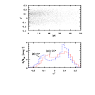
Figure 19: The dependence of asteroid color on the phase angle for 4591 asteroids with photometric errors less than 0.05 mag. in the $g^{\prime}$, $r^{\prime}$, and $i^{\prime}$ bands is shown in the top panel. The bottom panel shows the color distribution for 1150 asteroids observed close to opposition by the dashed line, and the color distribution for 1244 asteroids observed at large angles from the antisun by the solid line. The blue asteroids ($a^{*}<0$) are redder by $\sim 0.05$ mag when observed at large phase angles, while the color distribution for red asteroids ($a^{*}\geq 0$) widens for large phase angles, without a change in the median value.

We investigate the dependence of color $a^{*}$ on angle $\phi$ by comparing the color histograms for objects observed close to opposition and for objects observed at large $\phi$. The top panel in Figure 19 shows the $a^{*}$ color for 4591 asteroids with photometric errors less than 0.05 mag. in the $g^{\prime}$, $r^{\prime}$, and $i^{\prime}$ bands, as a function of the opposition angle $\phi$. The bottom panel shows the color distribution for 1150 asteroids observed close to opposition by the dashed line, and the color distribution for 1244 asteroids observed at large $\phi$ by the solid line. We find a significant difference in the $a^{*}-\phi$ relation for the two types of asteroids: the blue asteroids ($a^{*}<0$) are redder by $\sim 0.05$ mag when observed at large phase angles, while the color distribution for red asteroids ($a^{*}\geq 0$) widens for large phase angles, without a corresponding change of the median value. The same analysis applied to other colors shows that the dependence on $\phi$ is the strongest for the $g^{*}-r^{*}$ color, and insignificant for other colors. While the magnitude of this effect seems to agree with the value of 0.0015 mag deg^-1 observed for the Johnson $B-V$ color (Bowel & Lumme 1979), the difference in the behavior of the two predominant asteroid classes has not been previously reported.

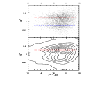
Figure 20: The color–absolute magnitude dependence for main belt asteroids. In the top panel each asteroid is shown as a dot, and in the bottom panel the distribution is outlined by isodensity contours. Two dashed lines are fitted separately for the $a^{*}<0$ and $a^{*}\geq 0$ subsamples. There is no significant correlation between the asteroid color and absolute magnitude.

Another effect which could bias the interpretation of the asteroid counts is the possible dependence of the asteroid color on absolute magnitude. Since for a given albedo the absolute magnitude is a measure of asteroid size, the dependence of the asteroid surface properties on its size could be observed as a correlation between the color and absolute magnitude. Figure 20 shows the distribution of asteroids in the color vs. absolute magnitude diagram for each color type separately (the top panel shows asteroids as dots, and the bottom panel shows isodensity contours). The absolute magnitude was calculated by using eq.9, and the heliocentric distance as described in Section 5.2. The two dashed lines are fitted separately for the $a^{*}<0$ and $a^{*}\geq 0$ subsamples. There is no significant correlation between the asteroid color and absolute magnitude (the slopes are consistent with 0, with errors less than 0.005 mag mag^-1).

6.3 The Absolute Magnitude and Heliocentric Distance Distributions

The differential counts of asteroids can be used to infer their size distribution if all asteroids have the same albedo. However, while the albedo within each of the two major asteroid types has a fairly narrow distribution (the scatter is $\sim$20% around the mean), the mean albedo for the two classes differs by almost a factor of 4 (Zellner 1979, Tedesco et al. 1989). The fact that the composition of the asteroid belt, and thus the mean albedo, varies with heliocentric distance has been a significant drawback for the determination of the size distribution (e.g. Jedicke & Metcalfe 1998). SDSS data can remedy this problem because the colors are sufficiently accurate to separate asteroids into the two classes. We assume in the following analysis that each color type is fairly well represented by a uniform albedo. We determine various distributions for each type separately, but also for the whole sample in order to allow comparison with previous work.

6.4 Determination of the Heliocentric Distance and Size Distributions

For a given apparent magnitude limit (here $r^{*}$= 21.5), the faint limit on absolute magnitude is a strong function of heliocentric distance (see e.g. eq. 1). For example, at $R$=2 AU, $r^{*}$=21.5 corresponds to $r^{*}$(1,0) = 19, while at $R$=3.5 AU, the limit is only 16.8. When interpreting the observed distribution of objects in the $r^{*}$(1,0) vs. $R$ plane, this effect must be properly taken into account. This problem is mathematically equivalent to the well studied case of the determination of the luminosity function for a flux limited sample (e.g. Fan et al. 2001b and references therein).

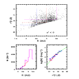
Figure 21: The top panel shows the dependence of absolute magnitude on heliocentric distance for blue asteroids. The three sets of lines mark boundaries of regions used to compute the heliocentric distance and absolute magnitude distributions shown in the bottom two panels (for details see text).

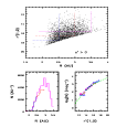
Figure 22: The same as previous figure except for red asteroids.

The top panels in Figures 21 and 22 show the $r^{*}$(1,0) vs. $R$ distribution of the two color-selected samples. We seek to determine the marginal distributions of sources in the $r^{*}$(1,0) and $R$ directions. It is usually assumed that these two distributions are uncorrelated (i.e. the $r^{*}$(1,0) distribution is the same everywhere in the belt, and the radial distribution is the same for all $r^{*}$(1,0)). The sample discussed here is sufficiently large to test this assumption explicitly, and we do so using two methods.

First, we simply define three regions in the $r^{*}$(1,0) vs. $R$ plane, outlined by different lines in the top panels, and compare the properly normalized histograms of objects for each of the two coordinates. If the distributions of $r^{*}$(1,0) and $R$ are uncorrelated, then all three histograms must agree. The results are shown in the bottom panels; the left panels show $R$ histograms, and the right panels show $r^{*}$(1,0) histograms (shown by points, the dashed lines will be discussed further below). In all four panels, the three histograms are consistent within errors (not plotted for clarity). That is, there is no evidence that the two distributions are correlated.

Another method to test for correlation between the two distributions is based on Kendall’s $\tau$ statistic (Efron & Petrosian 1992), and is well described by Fan et al. 2001b (see §2.2). For uncorrelated distributions the value of this statistic should be much smaller than unity. We find the values of 0.11 and 0.07, for the blue and red samples respectively, again indicating that $r^{*}$(1,0) and $R$ are uncorrelated.

The $R$ and $r^{*}$(1,0) distributions plotted in the bottom panels of Figures 21 and 22 are not optimally determined because they are based on only small portions of the full data set, and also suffer from binning. Lynden-Bell (1971) derived an optimal method to determine the marginal distributions for uncorrelated variables that does not require binning and uses all the data. We implemented this method, termed the $C^{-}$ method, as described in Fan et al. (2001b). The output is the cumulative distribution of each variable, evaluated at the measured value for each object in the sample. One weakness of this method is that the uncertainty estimate for the evaluated cumulative distributions is not available. We determine the differential distributions by binning the sample in the relevant variable, and assume the Poisson statistics based on the number of sources in each bin to estimate the errors.

6.5 The Asteroid Heliocentric Distance Distribution

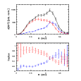
Figure 23: The top panel shows the relative surface density of asteroids as a function of heliocentric distance. The solid line corresponds to all asteroids, and the dashed and dot-dashed lines correspond to red and blue asteroids, respectively. The bottom panel shows the fractional contribution of each type in an absolute magnitude limited sample to the total surface density.

The top panel in Figure 23 shows the surface density of asteroids as a function of heliocentric distance. The surface density is computed as the differential marginal distribution in the $R$ direction, divided by $R$. The overall normalization is arbitrary and will be discussed in the next Section. The solid line corresponds to the full sample, the dashed line to red asteroids, and the dot-dashed line to blue asteroids. The relative normalization of the two types corresponds to samples limited by absolute magnitude. The distribution for the full sample is in good agreement with the results obtained by Jedicke & Metcalfe (1998, figure 3). In particular, the depletion of asteroids near $R=2.9$ spanning the range from the 5:2 to 7:3 mean motion resonance with Jupiter is clearly visible.

Figure 23 confirms earlier evidence (see e.g. Figure 17) that the heliocentric distance distributions of the two types of asteroids are remarkably different. This difference may be interpreted as two distinct asteroid belts: the inner belt dominated by red (S-like) asteroids, centered at $R$ $\sim$2.8 AU, with a FWHM of 1 AU, and the outer belt, dominated by blue (C-like) asteroids, centered at $R$ $\sim$3.2 AU, with a FWHM of 0.5 AU. This distinction is also motivated by the strikingly different radial shapes of the surface density. It may be possible to derive strong constraints on the asteroid history by modeling the curves shown in Figure 23, but this is clearly beyond the scope of this paper.

The distribution of red asteroids is fairly symmetric around $R\hbox{$\sim$}2.8$ AU, while the distribution of blue asteroids is skewed and extends all the way to $R\hbox{$\sim$}2$ AU. The overall shape indicates that it may represent a sum of two roughly symmetric components, with the weaker component centered at $R$ $\sim$2.5 AU, and the stronger component centered at $R$ $\sim$3.2 AU. Gradie & Tedesco (1982) showed that the distribution of M type asteroids has a local maximum around $R\hbox{$\sim$}2.5$ AU. Furthermore, these asteroids have colors similar to C type asteroids (see Figure 10) and can be distinguished only by their large albedo. Thus, it may be possible that $\lesssim 20\%$ of blue asteroids found at small $R$ ($\lesssim 3$ AU) are dominated by M type asteroids.

The bottom panel shows the fractional contribution of each type to the total surface density. The number ratio of the red to blue type changes from 4:1 in the inner belt to $\sim$1:3 in the outer belt (note that the number ratio for the outer belt has a large uncertainty). It should be emphasized that the amplitudes of the distributions of asteroids shown in the top panel, and thus the resulting number fractions, are strongly dependent on the sample definition. The plotted distributions, and the change of number fractions from 4:1 to 1:3, correspond to an equal cutoff in absolute magnitude. However, it could be argued that the cutoff should correspond to the same size limit. In such a case the red sample should have a brighter cutoff due to its larger albedo, which decreases its fractional contribution. For example, adopting a 1.4 mag brighter cutoff (see Section 4.1.2) for the red asteroids ($r^{*}$=20.1 instead of $r^{*}$=21.5) changes their fraction in the observed sample from 60% to 38%. We further discuss the number ratios of the two dominant asteroid types in the next two sections.

6.6 The Asteroid Absolute Magnitude Distribution

6.6.1 The Cumulative Distribution and Normalization

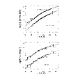
Figure 24: The top panel shows the cumulative luminosity functions for main belt asteroids, where the symbols correspond to the nonparametric estimates, and the lines are analytic fits to these estimates (see text). The solid lines and triangles correspond to asteroids with $a^{*}\geq 0$, and the dashed lines and circles to asteroids with $a^{*}<0$. The results for asteroids with $a^{*}\geq 0$ are multiplied by 10 for clarity. The two vertical lines close to $r^{*}$(1,0) = 18 correspond to asteroid diameter of 1 km. The bottom panel displays the differential luminosity function for main belt asteroids determined in this work (lines and error bars for analytic fits and nonparametric estimates, respectively), and the result by Jedicke & Metcalfe (1998) shown as open circles.

The top panel in Figure 24 shows the cumulative $r^{*}$(1,0) distribution functions (the total number of asteroids brighter than a given brightness limit) for main belt asteroids. The symbols (circles for asteroids with $a^{*}<0$ and triangles for asteroids with $a^{*}\geq 0$) show the nonparametric estimate obtained by the $C^{-}$ method (every asteroid contributes to the estimate and is represented by one symbol). The results for red asteroids are multiplied by 10 for clarity.

The counts are re-normalized to correspond to the entire asteroid belt by assuming that the belt does not have any longitudinal structure. This assumption is well supported by the data because the counts of main belt asteroids observed in the Spring and Fall subsamples agree to within their Poisson uncertainty ($\sim$1%). The normalization is determined by the counts of asteroids with $r^{*}$(1,0) $<$ 15.3, which is the faintest limit that is not affected by the apparent magnitude cutoff of the sample (see Figures 21 and 22). There are 337 blue and 519 red asteroids with $r^{*}$(1,0) $<$ 15.3, corresponding to 18,000 blue and 27,700 red asteroids in the entire belt. The multiplication factor (53.4) includes a factor of 2.03 to account for the $\phi$ cut (see Section 3.1) and the “uniqueness” cut (see Section 3.3), that decreased the initial sample of 10678 asteroids to the final sample of 5253 unique asteroids with reliable velocities. The remaining factor of 26.3 reflects the total area covered by the four scans analyzed here, that is, the data cover 3.8% of the Ecliptic.

The normalization uncertainty due to Poisson errors is about 5%. An additional similar error in the normalization may be contributed by the uncertainty in the estimated heliocentric distance, another comparable term by the uncertainty of absolute photometric calibration ($\lesssim 0.05$ mag), and yet another one by the uncertainty associated with defining a unique sample (see Section 3.3). Thus, the overall normalization uncertainty is about 10%.

Since the blue and red asteroids have different albedo, a $r^{*}$(1,0) limit does not correspond to the same size limit. To illustrate this difference, the two vertical lines close to $r^{*}$(1,0) = 18 mark asteroid diameter of 1 km; the cumulative counts are 370,000 for the blue type, and 160,000 for the red type.

The normalization obtained here is somewhat lower than recent estimates by Durda & Dermott (1997) and Jedicke & Metcalfe (1998). Durda & Dermott used the McDonald Survey and Palomar-Leiden Survey data (van Houten et al. 1970) and found that the number of main-belt asteroids with $H<15.5$ (absolute magnitude $H$ is based on the Johnson V band, $H$-$r^{*}$(1,0) $\sim$0.2) is 67,000. Jedicke & Metcalfe used the Spacewatch data and found a value of 120,000. As discussed above, the SDSS counts imply that there are 45,700 asteroids with $H<15.5$, or about 1.5 times less than the former, and 2.6 less than the latter estimate. Taking the various uncertainties into account, the normalization obtained in this work is marginally consistent with the results obtained by Durda & Dermott. We point out that the methods employed here to account for various selection effects are significantly simpler that those used in other determinations due to the homogeneity of the SDSS data set.

The nonparametric estimate shows a change of slope around $r^{*}$(1,0)$\sim$15-16 for both subsamples and suggests the fit of the following analytic function

$$N_{cum}=N_{o}{10^{ax}\over 10^{bx}+10^{-bx}},$$ (12)

where $x=\hbox{$r^{*}$}(1,0)-r_{C}$, $a=(k_{1}+k_{2})/2$, $b=(k_{1}-k_{2})/2$, with $k_{1}$ and $k_{2}$ the asymptotic slopes of log(N)-$r$ relations. This function smoothly changes its slope around $r^{*}$$\sim$$r_{C}$. The best fits for each subsample are shown by lines, and the best-fit parameters (also including the whole sample) are listed in Table 4 (note that the sum of the $N_{o}$ values for the blue and red subsamples is not exactly equal to the $N_{o}$ for the whole sample due to slightly varying $r_{C}$).

The red sample shows marginal evidence that the power-law index is smaller for $r^{*}$(1,0)$\lesssim$ 12.5 than for 12.5 $\lesssim$ $r^{*}$(1,0)$\lesssim$ 15. A best-fit power-law index for the 20 points with 10 $<$ $r^{*}$(1,0) $<$ 12.5 is 0.39$\pm$0.03. A few points at the bright end of the blue sample that could perhaps be interpreted as evidence for a similar change of slope have no statistical significance.

6.6.2 The Differential Distribution

The bottom panel in Figure 24 displays the differential luminosity distribution for main belt asteroids determined from the cumulative luminosity distribution by two different methods (the curves are shifted for clarity; the proper normalization can be easily reproduced using the best-fit parameters from Table 4). The lines show the analytic derivative of the best fit to the cumulative luminosity function (see eq. 12). The nonparametric estimates are determined by binning the sample in $r^{*}$(1,0) and piecewise fitting of a straight line to the cumulative distribution. The points are not plotted for clarity, and the displayed error bars are computed from Poisson statistics based on the number of objects in each bin. There is no significant difference between the results obtained by the two methods. The analytic curves are also shown in the bottom right panel of Figures 21 and 22.

The recent result for the asteroid differential luminosity function by Jedicke & Metcalfe (1998) is shown as open circles. Their estimate corresponds to the total sample because they did not have color information. Overall agreement between the two results is encouraging, given that the observing and debiasing methods are very different, and that they were forced to assume a mean asteroid albedo due to the lack of color information. Our result indicates that the turn over at the faint end that they find is probably not real, while the sample discussed here does not have enough bright asteroids (only $\sim$20) to judge the reality of the bump at the bright end. Nevertheless, it seems that the two determinations are consistent, and, furthermore, appear in qualitative agreement with results from the McDonald Asteroid Survey and the Palomar-Leiden Survey (van Houten et al. 1970).

6.7 The Asteroid Size Distribution

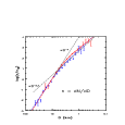
Figure 25: The differential size distribution normalized by its value for $D$=10 km (solid and dashed lines for analytic estimate, and error bars for nonparametric estimate, for red and blue asteroids respectively). The dot-dashed lines are added to guide the eye and correspond to power-law size distributions with index 4 and 2.3 (see text for discussion).

Assuming that all asteroids in a given sample have the same albedo, the differential luminosity function can be transformed to the size distribution with the aid of eq. 2 (note that the best-fit parameters listed in Table 4 fully describe the size distribution, too). Figure 25 shows the differential size distributions ($dN/dD$) normalized by the value for $D$=10 km (solid and dashed lines, for red and blue asteroids respectively). We have assumed albedos of 0.04 and 0.16 for the blue and red asteroids (see Section 4.1.3). Since the distributions are renormalized, these values matter only slightly in the region with $D$ $\sim$5 km where the size distributions change slope. The dot-dashed lines are added to guide the eye and correspond to power-law size distributions with index 4 and 2.3.

The agreement between the data for D $\gtrsim$ 5 km and a simple power-law size distribution with index 4 is remarkable. From eq. 7 and the best-fit values from Table 4, we find that the implied best-fit power-law index is 4.00$\pm$0.05 for both types. The power-law index of both asteroid types for D $\lesssim$ 5 km is close to 2.3, although there may be significant differences. The best fit values are 2.40$\pm$0.05 and 2.20$\pm$0.05 for the blue and red types, respectively. However, these error estimates do not account for possible hidden biases in the analysis. For example, a linear bias in the estimates of heliocentric distance (e.g. $R_{est}=0.95*R_{true}+0.1$, see Appendix B) would change the power-law index by about 0.03. Nevertheless, it is unlikely that such a bias would be different for the two types, and thus the difference in their power-law indices of 0.20 for D $\lesssim$ 1 km may be a real (4 $\sigma$) effect in the explored size range.

7 The Search for Asteroids by Combining SDSS and 2MASS Data

7.1 2MASS Data

The Two Micron All Sky Survey (2MASS, Skrutskie et al. 1997) is surveying the entire sky in near-infrared light. The observations are done simultaneously in the $J$ (1.25 $\mu{\rm m}$), $H$ (1.65 $\mu{\rm m}$), and $K_{s}$ (2.17 $\mu{\rm m}$) bands. The detectors are sensitive to point sources brighter than about 1 mJy at the $10\sigma$ level, corresponding to limiting (Vega-based) magnitudes of 15.8, 15.1, and 14.3, respectively. Point-source photometry is repeatable to better than 10% precision at this level, and the astrometric uncertainty for these sources is less than 0.2 arcsec. The 2MASS has observed $\sim$300 million stars, as well as several million galaxies, and covered practically the whole sky.

Moving objects cannot be recognized in 2MASS data without additional information. Such information is available for known asteroids and comets, and they are identified as a part of routine processing of the data (Sykes et al. 2000, hereafter S2000). The initial catalogs for about 3,000 deg² contain observations of 1054 asteroids and 2 comets. S2000 describe color-color diagrams for these asteroids and show that they span quite narrow ranges of $J-H$ and $H-K_{s}$ colors (about 0.2-0.3 mag. around $J-H$ $\sim$0.5 and $H-K$ $\sim$0).

7.2 Matching SDSS and 2MASS Data

We use SDSS data to find candidate asteroids in 2MASS data. SDSS can be used to detect moving objects in 2MASS catalogs because the two data sets were obtained at different times and thus SDSS should not detect positional counterparts to asteroids observed by 2MASS. The aim of this search is to detect asteroids with very red colors which may have been missed in optical surveys due to faint optical fluxes. For example, the unusual R-type (red) asteroid 349 Dembowska has a K-band albedo about 5 times larger than its $r^{\prime}$-band albedo (Gaffey, Bell & Cruikshank 1989). Since the solar $r^{\prime}$-K color is about 2 (Finlator et al. 2000, hereafter F00), a similar asteroid with $r^{\prime}$=15, which is roughly the completeness limit for cataloged asteroids, would have K=11 (here we used catalogued SDSS and 2MASS magnitudes; note that SDSS magnitudes are calibrated on an AB system, while 2MASS magnitudes are calibrated on Vega system, for details see F00). This is about 3 magnitudes brighter than the 2MASS faint cutoff in the K band, and shows that any significant population of red asteroids would be easily detected by combining SDSS and 2MASS data.

The positional matching of the sources observed by SDSS and 2MASS is described by F00 and Ivezić et al. (2001). Here we briefly summarize their results and extend these studies to search for asteroids among 2MASS Point Source Catalog (PSC) sources without optical counterparts.

F00 positionally matched the 2MASS PSC from the recent 2MASS Second Incremental Data Release to data from two SDSS fall commissioning runs (94 and 125, see Table 1) along the Celestial Equator extending from $\alpha_{J2000}$ = 0^h 24^m to $\alpha_{J2000}$ = 3^h 0^m and with $-1.2687^{\circ}<$ $\delta_{J2000}$ $<0^{\circ}$ (2MASS data for $\delta>0$ are not yet publicly available). The region with 1^h 51^m $<$ $\alpha_{J2000}$ $<$ 1^h 57^m is missing from the 2MASS catalog. The resulting overlapping area (47.41 deg²) includes 64,695 2MASS sources, and 97.9% of them are matched to a catalogued SDSS source to better than 2 arcsec. The inspection of SDSS images at the positions of unmatched 2MASS sources shows that in about 30% of cases (0.6% of the total) there is an SDSS source not listed in the catalog. They are usually associated with a saturated or very bright star ($\sim$1/2), with a complex blend of sources ($\sim$1/3), or with a diffraction spike or satellite trail. The remaining 1.4% unmatched 2MASS sources can be either

1. Moving objects

2. Extremely red sources (e.g. stars heavily obscured by circumstellar dust)

3. Spurious 2MASS detections

Since we are trying to maximize the number of candidate asteroids, we rematched the 2MASS PSC and SDSS catalogs in a larger region centered on the Ecliptic and observed in two SDSS spring commissioning runs (752 and 756, see Table 1) along the Celestial Equator. This region extends from $\alpha_{J2000}$ = 10^h 00^m to $\alpha_{J2000}$ = 14^h 00^m with $-1.2687^{\circ}<$ $\delta_{J2000}$ $<0^{\circ}$. The resulting overlapping area (76.07 deg²) includes 115,076 2MASS sources, and 98.57% of them are matched to a catalogued SDSS source to better than 2 arcsec. The inspection of SDSS images at the positions of 1641 unmatched 2MASS sources shows that in about 50% of cases (817, or 0.7% of the total) there is an SDSS source not listed in the catalog, in agreement with F00, and indicating that the completeness of the SDSS catalog at the bright end is $\sim$99.3%. The fraction of 2MASS sources without an optical counterpart (824, or 0.7%) is lower by about a factor of 2 for this sample than for the sample discussed by F00 (1.5%).

7.3 Analysis of 2MASS sources without Optical Counterparts

The sample of 824 2MASS sources without optical counterparts is a promising source of faint, unusual asteroids. To minimize the number of spurious 2MASS detections, we first analyze the statistics of 2MASS processing flags. In each 2MASS band, $rd\_flg$ indicates the quality of profile extraction, $bd\_flg$ indicates whether a source is blended, and $cc\_flg$ indicates whether the source’s photometry and position may be affected by artifacts of nearby bright stars or by confusion with other nearby sources. By using these flags we divide the sample into 5 categories listed in Table 5. We find that only 5.3% of sources have impeccable detections in all three 2MASS bands, while more than 80% of sources are detected only in J, or only in H. Because the objects do not have SDSS counterparts, the latter are probably spurious detections. We point out that the fraction of J-only and H-only detections in the 2MASS catalog is only 2.3%, as shown in the table. Thus, although the fraction of these, presumably spurious, detections is above 80% for the 2MASS sources without optical counterparts, these listings represent only 25% of the total number of such J-only and H-only detections (for H-only detections considered alone this fraction is 57%). Consequently, the 2MASS processing software was appropriately tuned to reach a reasonable compromise between the reliability and completeness of the J-band only detections.

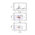
Figure 26: The color-magnitude and color-color diagrams for the candidate asteroids selected in 2MASS data. The top panel shows the K vs. J-K color-magnitude diagram for 42 reliable 2MASS PSC objects in the analyzed region without an SDSS counterpart within 3 arcsec. The 24 objects flagged as minor planets in the 2MASS database are shown as large dots, and the rest of objects are shown as open triangles. The middle panel shows the H-K vs. J-H color-color diagram for the same objects. The two contours outline the distribution of known asteroids, and enclose approximately 2/3 and 95% of sources from Sykes et al. (2000). The bottom panel shows H-K vs. J-H color-color diagram for the 9 objects with $K_{s}<14.3$ (10$\sigma$ limit).

We select the 42 objects with good detections in all 3 2MASS bands as plausible asteroid candidates. The $K_{s}$ vs. $J-K_{s}$ color-magnitude diagram and the $H-K_{s}$ vs. $J-H$ color-color diagram for these objects are shown in the top two panels in Figure 26. The 24 objects flagged by 2MASS as known minor planets are shown as large dots, and the others as open triangles. The two contours in the middle panel outline the distribution of the known asteroids, and enclose approximately 2/3 and 95% of sources from S2000. The bright sources predominantly have $J-K_{s}<1$ as shown by S2000. The sources outside the contour outlining the S2000 sample are predominantly faint and it is not clear whether they are scattered out by measurement errors, whether they are asteroids with peculiar colors, or whether they are asteroids at all. We find no strong correlation with the distance from the Ecliptic for these sources, but note that the sample is very small.

We further limit the sample by requiring at least 10$\sigma$ detection in the $K_{s}$ band ($K_{s}<14.3$), which automatically guarantees at least 10$\sigma$ detections in the other two bands (because asteroids are bluer than the colors of 2MASS N$\sigma$ limits). This requirement leaves 9 sources whose $H-K_{s}$ vs. $J-H$ color-color diagram is shown in the bottom panel in Figure 26. All of these are flagged as minor planets, showing that reliable 2MASS detections without SDSS counterparts are heavily dominated by previously known asteroids. Furthermore, to a magnitude limit of $r^{*}$=16.3, there are 24 asteroids in the analyzed area. This is in good agreement with the faint cutoff for SDSS-2MASS matched stars with $g^{*}-r^{*}$ color similar to asteroids (see F00, fig. 4), and indicates that the catalogued asteroids are complete to a similar depth, in agreement with Zappala & Cellino (1996). We conclude that there is no evidence for the existence of a significant population of asteroids with extremely red optical-IR colors, and estimate an upper limit of 10% for the fraction of extremely red asteroids which escaped detection at optical wavelengths.

It cannot be excluded that at least some asteroids have very peculiar IR colors. We have attempted to reobserve two sources selected from the sample of 2MASS sources without SDSS counterparts discussed by F00. These (2MASS 0041309-002730 and 2MASS 0053480-003836) were selected to have the most extreme near-infrared colors; the first has good detections in all 3 2MASS bands, and the second was detected only in the K band and flagged as an unreliable source. We used the United Kingdom Infrared Telescope UKIRT and the infrared array camera UFTI in J band on the night of Sept 21, 2000. We did not detect either object within UFTI’s 50 arcsec field of view to a limit of about 18 mag, implying that they are moving objects. Since the second source was already flagged as unreliable by 2MASS processing software, we consider only the first source as a good candidate for an asteroid with peculiar infrared colors (it is not flagged by 2MASS as a minor planet). Its 2MASS measurements are J=15.64$\pm$0.05, J-H=1.01$\pm$0.07, H-K=0.04$\pm$0.10.

S2000 discuss two asteroids with very peculiar colors and warn that they may be blends with a background object. However, this explanation is probably not applicable for this asteroid because there are no optical nor infrared sources at the position of the 2MASS detection. In principle, there could exist a very red and very variable source that was observed by 2MASS, and was not detected in UKIRT observation because it was in its faint phase. However, the probability for this seems very small.

8 The Search for the Kuiper Belt Objects

The Kuiper Belt Objects (KBOs, sometimes known as trans-Neptunian objects) are an ancient reservoir of objects located beyond Neptune’s orbit, which are believed to be the origin of short-period comets (Fernández 1980, Duncan, Quinn & Tremaine 1988; for a detailed review see Jewitt 1999). It is estimated that the number of the KBOs larger than $100$ km in diameter (assuming geometric albedo of 0.04) is $\sim 10^{5}$ in the $30$ to $50$ AU distance range (Jewitt 1999). The total mass in the KBOs is thought to be somewhat less than one Earth mass, and the expected sky density of the KBOs brighter than $r^{*}$$\sim$ 21.5 mag is about 0.01-0.04 deg^-2.

The first KBO was detected by Jewitt & Luu (1992), and today there are close to 300 known objects. Most of these are very faint: a KBO with radius equal to $\sim$100 km and albedo 0.04 has a visual magnitude of 22 at a distance of $\sim$30 AU from the Sun. Finding such objects poses quite a challenging task; to date detections have usually been accomplished by detecting their angular motion on the sky using large optical telescopes.

As discussed in Section 2.3, the KBOs move a bit too slowly to be detected in a single SDSS run. However, they can be detected by comparing two scans of the same area, as long as they are obtained within a week (otherwise a KBO would move to the region between two scanned columns). Here we describe a method developed for finding KBOs in two-epoch data and apply it to data for about 100 deg² of sky observed twice $\sim$ 1.9943 days apart (runs 745 and 756, see Table 1). The lower limit for detectable angular motion range is 0.0004 deg/day, and is set by a matching radius of 1 arcsec. The upper limit is determined by the maximum change in position for an object to be observed in both epochs and is about 0.08 deg/day. As the expected KBO motion is well within these limits, the only practical constraint is the brightness. The lower limit on KBO size to be detected with $\hbox{$r^{*}$}=22$ during oposition at a heliocentric distance of 40 AU is about 400 km (assuming an albedo of 0.04).

8.1 The Search Method

Slow moving objects like KBOs can be detected in two-epoch data because at each of the two observed positions they will not have a positional match in the other epoch. The probability of a random association with a background object is very low because the SDSS photometric pipeline deblends overlapping objects, unless they are too close to one another. Assuming a lower limit of 2 arcsec for a pair of nearby sources to be deblended, only $\hbox{$\sim$}10^{-3}$ of potential KBOs will be lost. The objects without positional counterparts in other epoch, hereafter called orphans, can then be matched within a much larger radius (a few arcmin) than the typical distance between two SDSS sources ($\sim$ 30 arcsec for $r^{*}$$\sim$ 22). Of course, there will also be orphans caused by instrumental effects such as diffraction spikes, satellite trails, seeing dependent deblending, etc. In addition to these, main-belt asteroids may be considered as contaminants when searching for KBOs.

Given a position of an orphan (i.e. a KBO candidate) in the first epoch, its position in the second epoch can be approximately predicted by assuming that the observed motion is due to Earth reflex motion and its own Keplerian proper motion. The predicted position depends on the time elapsed between the two observations, and object’s unknown heliocentric distance and orbital inclination. Because of the KBO’s proper motion, the region in the second epoch where a matching orphan would be found is an ellipse for each possible heliocentric distance, with its major axis parallel to the Ecliptic. Assuming observations close to opposition, the distance parallel to the Ecliptic between the center of this ellipse and the first position is

$$\Delta\lambda=0.9856{\Delta t\over R-1}\,\hbox{deg/day},$$ (13)

where $\Delta t$ is the elapsed time in days, and is determined by the Earth’s reflex motion. The major axis of this ellipse is given by

$$a={\Delta\lambda(R)\over\sqrt{R}},$$ (14)

and its minor axis by

$$b=a\cos(\beta).$$ (15)

An example of such ellipses for several different $R$ is shown in Figure 27. Since the distribution of possible distances is continuous, the overall search region assumes a wedge-like shape as shown in Figure 27. This shape is approximately described by

$$\Delta\beta=\pm{\cos(\beta)\Delta\lambda(R)\over\sqrt{R}}.$$ (16)

The pairs of orphans that are matched within such search box, determined for a range of plausible $R$ (assumed to be 10-300 AU), can still be spurious matches and we further require that each candidate pair of detections satisfy

1. No significant motion should be detected within a single run to avoid spurious matches with main-belt asteroids.

2. Both detections must be unresolved sources brighter than $r^{*}$=22, and must not be blended (objects with more than one peak) or saturated, nor cosmic rays.

3. The measured $g^{*}-r^{*}$ and $r^{*}-i^{*}$ colors for the two epochs must agree within 1$\sigma$ (the agreement between the two sets of magnitudes is not required because the brightness could vary if the object has irregular shape and rotates).

8.2 Results

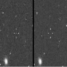
Figure 28: The KBO candidate observed in the first epoch. The left panel shows the 1x1 arcmin $r^{\prime}$-band image from run 745 with the position of the KBO marked by a cross. The right panel shows the same part of the sky observed in in the second epoch (run 756) with the same position marked by a cross. The images are assembled from the postage stamps for all objects detected by photometric pipeline.

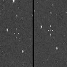
Figure 29: Same as the previous figure, except that the KBO candidate is observed in the second epoch.

We searched 99.5 deg² of sky observed twice 1.9943 days apart (runs 745 and 756, see Table 1) using the algorithm described in the previous section. The application of the first two criteria results in 166 candidate pairs, which are reduced to only 6 candidates by the application of the color constraint. We inspected visually 24 images corresponding to these 6 candidates and found that five candidates can be excluded as instrumental effects. The 4 images for the sixth candidate are shown in Figures 28 and 29.

The measured parameters for this KBO candidate are listed in Table 6, and the derived properties are listed in Table 7. Note that the magnitudes are the same within the measurement uncertainty, although this was not required by the algorithm, indicating that this object may have quite a regular shape. The candidate’s distance is obtained from its angular motion; it is multi-valued because the two-epoch data are insufficient to fully constrain the candidate’s orbital parameters. The ambiguity in distance propagates to the ambiguity in size.

We use the photometric transformations listed by Fukugita et al. (1996) to translate the KBO colors measured by other groups (Luu & Jewitt 1996; Tegler & Romanishin 1998) to the SDSS photometric system. We find that typical KBO colors are $g^{\prime}-r^{\prime}\approx 0.8\pm 0.3$ and $r^{\prime}-i^{\prime}\approx 0.4\pm 0.2$. The colors of the SDSS KBO candidate ($g^{*}-r^{*}$$\sim$1.0, $r^{*}-i^{*}$$\sim$0.5) fall within these ranges. As noted earlier, these colors are significantly redder than the colors of main-belt asteroids.

The search for KBOs is also sensitive to Centaurs, but we did not find any reliable candidates in the searched area.

8.3 Completeness of the search for KBOs

The third search criterion described above requires that the $g^{*}-r^{*}$ and $r^{*}-i^{*}$ colors must agree within 1$\sigma$ between the two observations, and decreases the number of candidates from 166 to 6. If this criterion is too conservative, then the number of detected KBOs could be 28 times higher.

We have tested this possibility by removing the third criterion and instead requiring that the observed $g^{*}-r^{*}$ color falls in the range 0.7-1.2 in both epochs (the left edge is 0.2 redder than discussed above due to the large increase in the number of stars with bluer colors). We also abandon any requirement on the orbit and simply match the orphans with required colors (120 and 300 from runs 745 and 756, respectively) within a circle with radius of 220 arcsec (corresponding to the motion of 0.03 deg day^-1).

We selected only one other candidate, and by visual inspection of images found that it was an instrumental effect. Thus we conclude that it is highly unlikely that our searching method missed any KBOs present in the data. It is not easy to precisely estimate this probability, but assuming that the most likely cause would be blending with another source, we place an approximate upper limit of 0.001 on the probability that there is another KBO which the search algorithm missed.

One detected source brighter than $r^{*}$=22 in 99.5 deg² is in agreement with expected density of 0.01-0.04 such objects per deg² (Jewit 1999). The significance of this result is limited by the small-number statistics.

9 Discussion

9.1 Moving Objects in SDSS

The detection of asteroids discussed in this work is based on a new algorithm, and thus it is of concern whether these sources really are asteroids. Based on the analysis presented here, the main arguments in favor of the reality of the SDSS detections are:

• Visual Inspection. But Yet They Move.

• The density of selected candidates correlates with the ecliptic latitude, although the position of the Ecliptic is not known to the algorithm, and the ecliptic latitude distribution width is consistent with observed distribution of known asteroids (see Sections 2.3 and 4.2.1).

• The color distribution of the selected candidates spans a much smaller range than that of stars, and corresponds to a G type star. Furthermore, it matches the colors of known asteroids observed with SDSS filters, and agrees with the synthetic colors derived from spectral data (see Section 4.1).

• The morphology of the velocity distribution for the selected candidates is in close agreement with the known orbital distribution of asteroids (see Section 5.1).

• For a limited area we show that the majority of candidates are recovered in a repeated scan (see Section 3.2).

The results presented here show that there are $\sim$530,000 objects larger than 1 km in the asteroid belt. This is about four times less than the previous estimates, e.g. the SIRTF planning for observing Solar System bodies assumes that there are as many as $2\times 10^{6}$ asteroids larger than 1 km (see Figure 4 in Hanner & Cruikshank 1999). As discussed in Section 6.6, about half of that discrepancy can be attributed to different normalizations, and the other half is probably due to smaller number of asteroids in the previously unexplored 1–5 km diameter range.

Extrapolating the observed asteroid density to the whole survey, we predict that by its completion SDSS will obtain about 100,000 near simultaneous five-color measurements for a subset drawn from 280,000 asteroids brighter than r $<$ 21.5 at opposition. While it is certain that a fraction of these observations will be multiple measurements of the same objects, the fraction cannot be estimated beforehand because it depends on the detailed observing strategy.

9.2 The Colors of Asteroids and the Heliocentric Distance Distribution

The color distribution of observed asteroids is strongly bimodal. While there is evidence for the existence of additional classes (see Sections 4.1.1 and 4.1.2), more than 98% of the objects in the sample have colors consistent with a simple separation into two basic color types. We find a significant correlation between asteroid colors and heliocentric distance, suggesting the existence of two distinct asteroid belts: the inner rocky belt, about 1 AU wide (FWHM) and centered at $R$ $\sim$2.8 AU, and the outer carbonaceous belt, about 0.5 AU wide and centered at $R$ $\sim$3.2 AU (see Sections 5.3 and 6.5). This result represents a significant constraint for the theories of Solar System formation (e.g. Ruzmaikina et al. 1989).

The correlation between the asteroid colors and their heliocentric distance has been recognized since the earliest development of taxonomies (for a historical overview see Gradie, Chapman & Tedesco 1989). The first evidence that various taxonomic types show distinct heliocentric distributions was presented by Chapman, Morrison & Zellner (1975) and later reinforced by using larger samples (Gradie & Tedesco 1982, Zellner, Tholen & Tedesco 1985). This study, which represents an increase in the sample size by more than a factor of 10, confirms that the number of red main belt asteroids decreases, and the number of blue main belt asteroids increases with the heliocentric distance. For samples defined by the same absolute magnitude cutoff, the number fraction of the red to blue asteroids varies from 4:1 at $R$ $\sim$2 AU, to about 1:3 at $R$ $\sim$3.5 AU. For sample defined by the same size cutoff, the number fraction of the red to blue asteroids is 1:2.3 for $D>1$ km (this ratio slightly depends on the size cutoff due to different size distributions). Our study has shown in addition that the surface number density of each type has a well defined maximum in the radial direction, and that the median color of each subsample becomes systematically bluer as the heliocentric distance increases.

The colors of Hungarias, Mars crossers, and near-Earth objects are more similar to the C-type than to S-type asteroids, suggesting that they originate in the outer belt. However, there are less than 50 objects in this sample and thus a larger data set is needed for a robust conclusion. We investigated the possibility that optical surveys are biased against very red asteroids by positionally matching the SDSS and 2MASS surveys. While we find one example of an asteroid with peculiar colors, there is no evidence for a significant fraction of very red asteroids ($\lesssim 10\%$).

9.3 The Asteroid Size Distribution

The size distribution discussed in Section 6.6 shows a striking change of the power-law index from 4 to $\sim$2.3 around $D$$\sim$5 km for both asteroid types. The steep slope applies up to the sample limit at $D$$\sim$40 km, and the shallow slope down to $D$$\sim$0.4 km. The dynamic range of $\sim$100 is the largest one obtained with a single data set.

In the first detailed study of the asteroid size distribution, Zellner (1979) found the power-law index $\alpha\hbox{$\sim$}(1.5-2)$ for asteroids larger than $\sim$ 20 km, corresponding to $r^{*}\lesssim 12$ where the counts analyzed in this study are limited by small-number statistics. Thus, our results are not in direct conflict with those obtained by Zellner, and may be considered the extension of the size distribution to smaller asteroid sizes. While it is conspicuous that the change from Zellner’s shallower size distribution to the steeper one obtained here occurs at the magnitude where the data samples barely overlap, the flattening of the size distribution for $D>20$ km is supported by more recent determinations. Using a sample of about 4000 asteroids, Cellino et al. (1991) found that the asteroid size distribution resembles a power law with index $\alpha\hbox{$\sim$}3$ for $D\gtrsim 150$ km, and becomes flatter for smaller sizes ($\alpha\hbox{$\sim$}1$), down to their sample size limit of 44 km. The results presented here are roughly consistent with a recent result for the absolute magnitude distribution by Jedicke & Metcalfe (1998) (shown as open circles in the bottom panel in Figure 25). A most notable difference in the region of overlap is that we do not detect the turn-over in the counts at the faint end (we detect about 2-3 times more objects in the relevant range of magnitudes, $r^{*}$(1,0) $\sim$16-17, or $r^{*}$$\lesssim$ 19).

It may be of interest to note that the size distribution for KBOs larger than $\sim$100 km seems to follow the $D^{-4}$ power law (Jewitt 1999), while the size distribution of comets appears to follow the $D^{-3}$ power law (Shoemaker & Wolfe 1982). The simulations of the asteroid belt evolution predict slopes similar to those detected here which range from 2.5 to 4.0 (Gradie, Chapman & Tedesco 1989), depending on detailed assumptions and modelled effects. For example, the $D^{-3.5}$ power law is expected to be produced by shattering collisions (Dohnanyi 1969, Williams & Wetherill 1994). The Jedicke & Metcalfe result for the absolute magnitude distribution was transformed into a size distribution and modeled by Durda, Greenberg & Jedicke (1998). They join the resulting distribution with the data for catalogued asteroids and find two “humps”: the first spans the range 30-300 km and the second spans the range 3-30 km (see their figure 2). These “humps” were explained by tailoring a detailed dependence of the critical specific energy (energy per unit mass required to fragment an asteroid and disperse the fragments to infinity) on asteroid size.

The size distributions derived here and shown in Figure 23 are smooth, and apart from the change in slope around D $\sim$5 km, do not show any structure. The discrepancies in the region of overlap with studies quoted above are probably due to different methods of correcting for selection effects. They were forced to assume a mean albedo due to the lack of color information, a problem that is alleviated by SDSS data. Due to significant differences in the mean albedo and radial density distribution of the two classes, this assumption may lead to biases, as was already pointed out in those studies. The same explanation can be invoked to account for the fact that, contrary to previous studies (e.g. Jedicke & Metcalfe 1998), we find no evidence that the size distribution varies with the heliocentric distance.

The SDSS data indicate that the size distribution of main belt asteroids is well described by a $D^{-4}$ power-law for 5 km $\lesssim D\lesssim$ 40 km, and by a $D^{-2.3}$ power-law for 0.4 km $\lesssim D\lesssim$ 5 km. Similar broken power laws have already been proposed for the size distribution of various solar system objects (e.g. Levison & Duncan 1990, Tremaine 1990), and in particular for the main-belt distribution (Cellino et al. 1991). While we don’t yet have an understanding of the processes responsible for the observed change of slope of size distribution from 4 to 2.3, it seems plausible that they could be modeled as in e.g. Durda, Greenberg & Jedicke (1998).

9.4 The Asteroid-Earth Impact Rates

A decrease by a factor of 4 in the estimated number of asteroids with $D>1$ km discussed here implies a similar decrease in estimates of various other quantities proportional to the number of asteroids, e.g. the contamination rate by asteroids when searching for stellar occultations by KBOs (C. Alcock, priv. comm.), and the frequency of “killer asteroids”, usually defined as objects larger than 1 km. The results presented here imply that the time until the next catastrophic asteroid collision with the Earth may be at least four times longer than previously thought (estimated to be $1-2\times 10^{5}$ years for objects larger than 1 km, see e.g. Spaceguard Survey Workshop Report, Verschuur 1991, Steel 1997, Ceplecha et al. 1998, Rabinowitz et al. 2000). Of course, the estimates of such impact rates based on the number of asteroids and dynamical considerations are rather uncertain, so it may be more robust to determine them from the historical impact records. On the other hand, the latter method suffers greatly from the small number statistics and unknown sample completeness.

The only known catastrophic event with a reliable estimate of the object size is the impact of a 10$\pm$4 km body that probably caused the extinction of dinosaurs 65$\pm$0.1 million years ago (Alvarez et al. 1980, van den Bergh 1994). Tying this impact rate ($\sim$1 per 10⁸ years for objects larger than 10 km) to the impact rate for objects larger than 1 km that are capable of causing global catastrophes, was until now based on the extrapolations of the size distribution. SDSS measurements for the first time reliably show that the number ratio of $D>$ 1 km asteroids and $D>$ 10 km asteroids is about 100, implying an impact rate for “killer asteroids” of about 1 every 10⁶ years, or at least several times less frequently than previous estimates. While still dependent on rather uncertain normalization, this estimate no longer relies on the extrapolation of the asteroid size distribution. Figure 30 shows that such an extrapolation overestimates the number of $D>$ 1 km asteroids by about a factor of 10.

9.5 Future Work

This work analyzes only 10% of the total number of asteroids to be observed by SDSS. Although this sample represents more than an order of magnitude increase in the number of asteroids with accurate multi-color photometry, another increase by factor of ten will be possible soon. With such massive and detailed information, it may be possible to develop a more sophisticated taxonomic scheme than attempted here, as well as to perform other types of studies; for example detailed modeling of the dependence of color on phase angle.

The main shortcoming of SDSS data for asteroid studies is insufficient information to determine orbits. Although the completeness of the catalogued asteroids is significant only at the bright end of the SDSS sample, the matching of known asteroids to SDSS observations would increase the sample of objects with both known orbits and accurate multi-color photometry by at least an order of magnitude. Additionally, about 225 deg² of the sky along the Celestial Equator will be surveyed dozens of times, and depending on the frequency of the observations, it may be possible to determine the asteroid orbits. These data will also be invaluable when searching for KBOs as described in Section 8.

We hope that this preliminary analysis will motivate further studies of the solar system using SDSS data. In particular, most of the data discussed here are part of the June 2001 SDSS Early Data Release.

Acknowledgments

We are grateful to Scott Tremaine, Mario Jurić, Dejan Vinković and Tim Knauer for their careful reading and insightful comments.

The Sloan Digital Sky Survey (SDSS) is a joint project of The University of Chicago, Fermilab, the Institute for Advanced Study, the Japan Participation Group, The Johns Hopkins University, the Max-Planck-Institute for Astronomy, New Mexico State University, Princeton University, the United States Naval Observatory, and the University of Washington. Apache Point Observatory, site of the SDSS telescopes, is operated by the Astrophysical Research Consortium (ARC).

Funding for the project has been provided by the Alfred P. Sloan Foundation, the SDSS member institutions, the National Aeronautics and Space Administration, the National Science Foundation, the U.S. Department of Energy, Monbusho, and the Max Planck Society. The SDSS Web site is http://www.sdss.org/.

This publication makes use of data products from the Two Micron All Sky Survey, which is a joint project of the University of Massachusetts and the Infrared Processing and Analysis Center/California Institute of Technology, funded by the National Aeronautics and Space Administration and the National Science Foundation.

Appendix A: Determination of Asteroid Heliocentric Distance from its Proper Motion

Following Jedicke (1996), we derive the following expressions which relate the observed ecliptic latitude, $\beta$, opposition angle $\phi$ (angular distance from the antisun), and the ecliptic velocity components, $v_{\lambda}$ and $v_{\beta}$, to the semimajor axis $a$ (or heliocentric distance $R$ because circular orbits are assumed), orbital inclination $i$, the longitude of the ascending node $\Omega$, and the rate of the radial motion $\dot{\Delta}$.

The heliocentric velocity vector of an asteroid is the composition of its relative velocity with respect to the Earth and the reflex motion of the Earth

$${\bf v}={\bf v}_{\rm rel}+{\bf v}_{\oplus},$$ (1)

where ${\bf v}_{\oplus}$ is the Earth’s velocity ($\|{\bf v}_{\oplus}\|=v_{E}=0.986$ deg day^-1). Since the orbits are assumed circular (for the Earth’s motion this is quite a decent approximation), the expressions for three vector components plus the norm of Eq. 1 yield a set of four equations with four unknowns ($R$, $i$, $\Omega$ and $\dot{\Delta}$).

$${\bf v} = {v_{E}\over\sqrt{R}}\left(\begin{array}[]{c}-\cos b\sin l\cos i-\sin b\cos\Omega\sin i\\ \cos b\cos l\cos i-\sin b\sin\Omega\sin i\\ \cos b\sin i(\cos l\cos\Omega+\sin l\sin\Omega)\end{array}\right)$$ (5)

$$= \left(\begin{array}[]{c}-\Delta(v_{\beta}\sin\beta\cos\phi+v_{\lambda}\sin\phi)+\dot{\Delta}\cos\beta\cos\phi\\ \Delta(v_{\lambda}\cos\phi-v_{\beta}\sin\beta\sin\phi)+\dot{\Delta}\cos\beta\sin\phi+v_{E}\\ \Delta v_{\beta}\cos\beta+\dot{\Delta}\sin\beta\end{array}\right)$$ (9)

$$\|{\bf v}\| = \Delta^{2}(v_{\lambda}^{2}+v_{\beta}^{2})+\dot{\Delta}^{2}+v_{E}^{2}$$ (10)

$$+2v_{E}\left[\Delta\left(v_{\lambda}\cos\phi-v_{\beta}\sin\beta\sin\phi\right)+\dot{\Delta}\cos\beta\sin\phi\right]$$

$$= {v_{E}\over\sqrt{R}},$$

where $(l,b)$ represent the heliocentric ecliptic longitude and latitude and $\Delta$ is the distance between the Earth and the object

$$\tan l = \frac{\Delta\cos\beta\sin\phi}{1+\Delta\cos\beta\cos\phi}$$ (11)

$$\tan b = \frac{\Delta\sin\beta(\sin l+\cos l)}{1+\Delta\cos\beta(\sin\phi+\cos\phi)}$$ (12)

$$\Delta = \sqrt{\cos^{2}\beta\cos^{2}\phi+R^{2}-1}-\cos\beta\cos\phi.$$ (13)

These equations are not invertible and we solve them by an iterative procedure based on routine newt.c from Numerical Recipes (Press et al. 1992).

The analysis of the accuracy of this method is described in Appendix B. It is noteworthy that somewhat simpler set of equations involving only two unknowns ($R$ and $i$) can be derived by utilizing the Cartesian coordinates and introducing several additional assumptions (Jedicke 1996).

$$v_{\lambda} = \sin(\phi){v_{x}\over\Delta}+\cos(\phi){v_{y}-v_{E}\over\Delta},$$

$$v_{\beta} = -\sin(\beta)\cos(\phi){v_{x}\over\Delta}+\sin(\beta)\sin(\phi){v_{y}-v_{E}\over\Delta}+$$ (14)

$$\cos(\beta){v_{z}\over\Delta},$$

where

$$\theta = \phi-{\rm arcsin}\left({\sin(\phi)\over R}\right)$$

$$\Delta = [R^{2}+1-2R\cos(\theta)]^{1/2}$$

$$v_{x} = {v_{E}\over R^{1/2}}\cos(i)\sin(\theta)$$

$$v_{y} = {v_{E}\over R^{1/2}}\cos(i)\cos(\theta)$$

$$v_{z} = {v_{E}\over R^{1/2}}\sin(i).$$ (15)

For small $\phi$ and $i$ ($\lesssim 10^{\circ}$), we find that this simplified set of equations performs as well as the first set of equations. For larger $\phi$ and $i$ its performance deteriorates.

Appendix B: Tests of the Algorithms By Using Database of Catalogued Asteroids

Many of the results presented in this work involve the asteroid heliocentric distance determined as described in Appendix A. Here we determine errors for the estimated values of heliocentric distance for a sample of asteroids with known orbits.

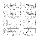
Figure 31: The accuracy of orbital elements determined from proper motions. For details see Appendix B.

We utilized the largest available database with orbital parameters for 114,539 asteroids provided by Bowell, Muinonen & Wasserman (1994). The positions of all asteroids were generated by a simple 2-body ephemeris generator for September 21, 1998, and March 21, 1999, and 1729 asteroids were selected in the observed area with $|\phi|<15^{\circ}$. This number corresponds to 28% of the number density observed by SDSS in the same area and selected with the same criteria. The asteroid proper motions were determined by computing the positions 288 seconds later and expressing the linear velocity in equatorial coordinates, as was done with the SDSS observations. These simulated observations were then processed by the same software as used in the analysis of the SDSS observations, producing a list of estimated semi-major axes and heliocentric distances, $a$ and $R$ ($a=R$), and orbital inclinations ($i$). Note that this procedure is an end-to-end test of the analysis pipeline (i.e. test of all the steps after detecting asteroids by the SDSS photometric pipeline). We determine the accuracy of the estimated values by comparing them to the known true values. The results are summarized in Figure 31.

The top left panel shows the difference between the estimated and true semi-major axis plotted vs. the true value, with each asteroid shown as a dot (note that estimate for $a$ is the same as estimate for $R$). The Kirkwood gaps are clearly visible in the distribution of semi-major axes. The mean error is correlated with the semi-major axis and we correct for this effect by fitting a straight line, producing the “best” estimate $a_{best}=a_{app}(1.085-0.03a_{app})$. The left panel in the second row shows the difference between this new value and true semi-major axis plotted vs. the true value, and the left panel in the third row shows the histogram of this difference. Its equivalent Gaussian width is only 0.072 AU, showing that the semi-major axis can be determined to within $\sim$3% although the method assumes circular orbits. This is the “intrinsic” accuracy of the method based on true proper motion. The errors in SDSS measurements will result in a wider distribution and we model this effect by adding errors with random amplitude of $\pm$5% to the true velocity. The added errors increase the width of $a_{best}-a_{true}$ distribution to 0.102 AU (the identical transformation from the “approximate” to “best” value was used).

The assumption of a circular orbit results in identical estimates of semi-major axis and heliocentric distance. The heliocentric distance is thus inevitably underestimated due to the eccentric orbits of asteroids (the mean orbital value of $R/a$ is greater than unity for an eccentric Keplerian orbit). This effect is visible in the upper right panel of Figure 31 which shows the difference between the approximate and true heliocentric distance plotted vs. the true value, where each asteroid is shown as a dot. We apply the same correction procedure as for the major axis estimate, resulting in a best estimate of $R_{best}=R_{app}(1.16-0.03R_{app})$ (which was used in the data analysis). The right panel in the second row shows the difference between this best value and the true value plotted vs. the true value, and the right panel in the third row shows the histogram of this difference. Its equivalent Gaussian width is 0.28 AU, about 4 times larger than the width of the corresponding distribution for the semi-major axis estimate.

Although the inclination estimate is not used quantitatively here, we also study its accuracy for completeness. The uncertainty of the inclination estimate is 17% with a bias of -7.8% (note that these values refer to fractional errors). The relevant diagrams are shown in the bottom row of Figure 31.

It is somewhat counterintuitive that the semi-major axis can be determined with about 4 times better accuracy than the heliocentric distance. After all, the main component of the asteroid proper motion is due to the Earth’s reflex motion which depends only on the asteroid distance. To illustrate how this apparent contradiction arises, it is sufficient to consider an asteroid observed at opposition, whose orbit has eccentricity $e$ and orbital inclination $i$=0^∘. In such a case, the observed angular velocity is

$$v_{\lambda}={v_{ast}-v_{E}\over R-1},$$ (16)

where

$$v_{ast}={v_{E}\over R}\sqrt{a(1-e^{2})}.$$ (17)

The semi-major axis and heliocentric distance are related by

$$R={a(1-e^{2})\over 1+e\cos{\Psi}},$$ (18)

where $\Psi$ is the true anomaly, which specifies the orientation of the orbit relative to the observer. Two limiting cases are perihelion ($\Psi=0^{\circ}$) and aphelion ($\Psi=180^{\circ}$). For fixed $a$ and $e$, the observation in perihelion corresponds to the smallest $R$ and the largest $v_{ast}$, while the opposite is true for observation in aphelion. The changes of $a$ and $R$ have opposite effects on $v_{\lambda}$ (note that $v_{E}>v_{ast}$), and this compensation results in a very minor dependence of $v_{\lambda}$ on unknown $\Psi$. We find that for the relevant range of parameters (2.2 $<a<$ 3.2, $e\lesssim 0.2$) the change of $v_{\lambda}$ is $\lesssim 3\%$ when $\Psi$ is varied from $0^{\circ}$ to 180^∘. Or equivalently, for a fixed (i.e. measured) $v_{\lambda}$, the uncertainty of $a$ is about 3% due to nonzero eccentricity (as found empirically). Note that even if the eccentricity were known (and nonzero, of course), this uncertainty would not be smaller because the problem is in unknown $\Psi$. Similarly, the larger uncertainty in $R$ is the result of random orientations of eccentric asteroid orbits. Even if all asteroid orbits had identical known eccentricity, the resulting uncertainty would be similar because the heliocentric distance can be anywhere between $R_{min}=(1-e)a$ and $R_{max}=(1+e)a$.

Table 1: SDSS commissioning runs used in this study

Runa	Dateb	Min. R.A.c	Max. R.A.d	Min. $\beta^{e}$	Max. $\beta^{f}$	Areag
94	1998-09-19	22h 25’	03h 46’	-20	5	100.9
125	1998-09-25	23h 21’	05h 07’	-20	5	97.5
752	1999-03-21	09h 40’	16h 46’	-14	20	133.9
756	1999-03-22	07h 50’	15h 44’	-14	20	149.3
1336h	2000-04-04	16h 43’	03h 29’	73	86	16.2
745-756i	1999-03-20	10h 42’	15h 46’	-8	20	97.5

Table 2: Classification regions in the $v_{\lambda}$ - $v_{\beta}$ diagram.

Region	velocity (deg/day)	angle (deg)	N ($r^{*}$$<$20.0)	N ($r^{*}$$<$21.5)
main belt	0.14 – 0.35	135 – 225	1718	5125
Hildas	0.14 – 0.18	175 – 185	11	59
Trojans	0.07 – 0.14	135 – 225	1	2
Centaurs	0.03 – 0.07	135 – 225	1	2a
Hungarias	0.35 – 0.50	90 – 135b	13	25
Mars crossers	0.35 – 0.50	135 – 150b	0	7
NEOs	0.35 – 0.50	150 – 210c	8	19
Unknown	0.35 – 0.50	90 – 135b	2	14
Total	—	—	1754	5253

Table 3: Parameters for broken power-law fits to main belt asteroid counts.

Parameter	$a^{*}<0$	$a^{*}>0$
$r_{b}$a	18.0	18.5
k${}_{B}^{b}$	0.69	0.52
k${}_{F}^{c}$	0.34	0.27
$\alpha_{B}^{d}$	4.5	3.6
$\alpha_{F}^{e}$	2.7	2.4

Table 4: Parameters for fits to the cumulative distributions of absolute magnitudes.

Parametera	$a^{*}<0$	$a^{*}>0$	all
$N_{o}$	44,300	74,000	111,600
$r_{C}$	15.5$\pm$0.01	15.6$\pm$0.01	15.5$\pm$0.01
k1	0.61$\pm$0.01	0.61$\pm$0.01	0.61$\pm$0.01
k2	0.28$\pm$0.01	0.24$\pm$0.01	0.25$\pm$0.01

Table 5: The flag statistics for 2MASS sources without optical matches.

Typea	rd_flg	bl_flg	cc_flg	Nb	%c	N${}_{all}^{d}$	%${}_{all}^{e}$
impeccable	222	111	000	42	5.1	93050	80.86
J-only	200	100	000	461	56.0	2325	2.02
H-only	020	010	000	211	25.6	368	0.32
K-only	002	001	000	17	2.1	81	0.07
all other	…	…	…	93	11.2	19252	16.73

Table 6: Measured parameters for the KBO candidate.

Parameter	Run 745	Run 756
RA	$193.63749^{\circ}$	$193.59462^{\circ}$
Dec	$-0.56884^{\circ}$	$-0.55040^{\circ}$
MJD-51,000	257.33775	259.33200
$\lambda$	$192.77092^{\circ}$	$192.72408^{\circ}$
$\beta$	$-5.05787^{\circ}$	$-5.05827^{\circ}$
u∗	$23.66\pm 0.59$	$23.49\pm 0.54$
g∗	$22.47\pm 0.11$	$22.40\pm 0.11$
r∗	$21.41\pm 0.07$	$21.42\pm 0.06$
i∗	$20.94\pm 0.07$	$20.95\pm 0.06$
z∗	$20.65\pm 0.20$	$20.90\pm 0.21$
g∗-r∗	$1.06$	$0.98$
r∗-i∗	$0.47$	$0.47$
a∗	$0.60$	$0.53$

Table 7: Derived parameters for the KBO candidate.

Parameter	Value
$v_{\lambda}$	-0.0235 deg/day
$v_{\beta}$	0.0002 deg/day
distance	36-49 AU
radius for:
albedo=0.04	210-390 km
albedo=0.25	80-150 km

Figure 1: The SDSS footprint in ecliptic coordinates. The survey avoids the Galactic plane and is limited to the area with Galactic latitude $b>30^{\circ}$ (approximately). The survey is performed by scanning along great circles indicated by solid lines. The position of the North Galactic Pole is indicated by an asterisk. The disconnected stripe that crosses $\lambda=0^{\circ}$ is the Southern strip. The shaded regions represent areas analyzed in this work.

Figure 27: The construction of the search box for matching moving objects observed in two different runs. Axes show the change in ecliptic coordinates between the two observations. An object at a given heliocentric distance would be found in one of the ellipses, with the exact position depending on the orientation of its proper motion vector. Different ellipses correspond to varying distances from 20 AU to 70 AU. Note that the orbital parameters constrained by an observed position are degenerate since any position can belong to more than one ellipse.

Figure 30: The solid line shows the estimate for asteroid impact rates with the Earth based on the asteroid size distribution determined here. The overall normalization is tied to the impact of a 10 km large body that caused the extinction of dinosaurs 65 million years ago. The dot-dashed line shows that extrapolation of the size distribution from the $D\hbox{$\sim$}10$ km end results in erroneous impact rate estimate for smaller objects.

References

- Allen (1973) Allen, C.W. 1973, Astrophysical Quantities (London: Athlone Press, 1973)
- Alvarez et al. (1980) Alvarez, L.W., Alvarez, W., Asaro, F. & Michel, H.V. 1980, Science, 208, 1095
- Bell (1989) Bell, J.F., Davis, D.R., Hartmann, W.K. & Gaffey, M.J. 1989, in Asteroids II, eds. R.P. Binzel, T. Gehrels and M.S. Matthews, (Tucson: Univ. of Arizona Press), 921
- Binzel (1989) Binzel, R.P. 1989, in Asteroids II, eds. R.P. Binzel, T. Gehrels and M.S. Matthews, (Tucson: Univ. of Arizona Press), 3
- Bowell & Lumme (1979) Bowell, E. & Lumme, K. 1979, in Asteroids, ed. T. Gehrels, (Tuscon: Univ. of Arizona Press), 132
- Bowell, Skiff, Wasserman & Russell (1989) Bowell, E., Skiff, B.A., Wasserman, H. & Russell K.S, 1989, in Asteroids, Comets, and Meteors III, eds. C.I. Lagerkvist, H. Rickman, B.A. Lindblad, and M. Lindgren (Uppsala University, Uppsala), 19
- Bowell, Muinonen & Wasserman (1994) Bowell, E., Muinonen, K., & Wasserman, H. 1994, A public-domain asteroid orbit database, In Asteroids, Comets, Meteors 1993, eds. Milani, A., et al., (Dordrecht: Kluwer Academic), 477
- Cellino et al. (1991) Cellino, A., Zappala, V., Farinella, P. 1991, MNRAS, 253, 561
- Ceplecha et al. (1998) Ceplecha, Z., et al. 1998, Space Science Reviews, 84, 327.
- Chapman, Morrison & Zellner (1975) Chapman, C.R., Morrison, D. & Zellner, B. 1975, Icarus, 25, 104
- Dermott, Gradie & Murray (1985) Dermott, S.F., Gradie, J., & Murray, C.D. 1985, Icarus 62, 289
- Dohnanyi (1969) Dohnanyi, J. 1969, J. Geophys. Res., 74, 2531
- Duncan, Quinn & Tremaine (1988) Duncan, M., Quinn, T., & Tremaine, S. 1988, ApJ, 328, L69
- Durda & Dermott (1997) Durda, D.D., & Dermott, S.F. 1997, Icarus, 130, 140
- Durda, Greenberg & Jedicke (1998) Durda, D.D., Greenberg, R., & Jedicke, R. 1998, Icarus, 135, 431
- Efron & Petrosian (1992) Efron, B. & Petrosian, V. 1992, ApJ, 399, 345
- Fan (1999) Fan, X. 1999, AJ, 117, 2528
- (18) Fan, X., et al. 2001a, AJ, 121, 31
- (19) Fan, X., et al. 2001b, AJ, 121, 54
- Fernández (1980) Fernández, J. 1980, MNRAS, 192, 481
- Finlator (2000) Finlator, K., et al. 2000, AJ, 120, 2615
- Fukugita et al. (1996) Fukugita, M., Ichikawa, T., Gunn, J.E., Doi, M., Shimasaku, K., & Schneider, D.P. 1996, AJ, 111, 1748
- Gaffey, Bell & Cruikshank (1989) Gaffey, Bell & Cruikshank 1989, in Asteroids II, eds. R.P. Binzel, T. Gehrels and M.S. Matthews, (Tucson: Univ. of Arizona Press), 117
- Gehrels (1979) Gehrels, T. 1979, in Asteroids, ed. T. Gehrels, (Tuscon: Univ. of Arizona Press), 3
- Gradie & Tedesco (1982) Gradie, J., & Tedesco, E.F. 1982, Science, 216, 1405
- Gradie, Chapman & Tedesco (1988) Gradie, J., Chapman, C.R., & Tedesco, E.F. 1989, in Asteroids II, eds. R.P. Binzel, T. Gehrels and M.S. Matthews, (Tucson: Univ. of Arizona Press), 316
- Gradie, Chapman & Williams (1988) Gradie, J., Chapman, C.R., & Williams, J.G. 1979, in Asteroids, ed. T. Gehrels, (Tuscon: Univ. of Arizona Press), 359
- Gunn et al. (1998) Gunn, J.E., et al. 1998, AJ, 116, 3040
- Hanner & Cruikshank (1999) Hanner, M.S. & Cruikshank, D.P. 1999, The Solar System and Circumstellar Dust Disks: Prospects for SIRTF, Report of a Workshop, August 18-20, 1999, Dana Point, California, available as http://sirtf.caltech.edu/SciUser/A_GenInfo/SSC_A4_DANA1999.html
- Hapke (1989) Hapke, B., Dominigue, D., Lumme, K., Peltoniemi, J. & Harris, A.W. 1989, in Asteroids II, eds. R.P. Binzel, T. Gehrels and M.S. Matthews, (Tucson: Univ. of Arizona Press), 524
- Ivezić & Elitzur (2000) Ivezić, Ž., & Elitzur, M. 2000, ApJ, 534, 93.
- Ivezić et al. (1999) Ivezić, Ž., et al. 2000, AJ, 120, 963
- Ivezić et al. (2001) Ivezić, Ž., et al. 2001, in prep.
- Jedicke (1996) Jedicke, R. 1996, AJ, 111, 970
- Jedicke & Metcalfe (1998) Jedicke, R., & Metcalfe, T.S. 1998, Icarus 131, 245
- Jewitt (1999) Jewitt, D. 1999, Annu. Rev. Earth. Planet. Sci, 27, 287
- Jewitt & Luu (1992) Jewitt, D., & Luu, J. 1992, Nature, 362, 730
- Kowal (1989) Kowal, C. 1989, Icarus, 77, 118
- Krisciunas, Margon & Szkody (1998) Krisciunas, K., Margon, B., & Szkody P. 1998, PASP 110, 1342
- Kuiper et al. (1958) Kuiper G.P., et al. 1958, ApJS 3, 289.
- Levison & Duncan (1990) Levison, H., & Duncan, M. 1990, AJ, 100, 1669
- Lupton, Gunn & Szalay (1999) Lupton, R.H., Gunn, J.E., & Szalay, A. 1999, AJ, 118, 1406
- Lupton et al. (2001) Lupton, R.H., et al. 2001, in preparation
- Luu & Jewitt (1996) Luu, J., & Jewitt, D. 1996, AJ, 112, 2310
- Lynden-Bell (1971) Lynden-Bell, D. 1971, MNRAS, 155, 95
- Muinonen, Bowell & Lumme (1995) Muinonen, K., Bowell, E. & Lumme, K. 1995, A&A, 293, 948
- Oke & Gunn (1983) Oke, J.B., & Gunn, J.E. 1983, ApJ 266, 713
- Pier et al. (2000) Pier, J.R., et al. 2001, in preparation
- Press et al. (1992) Press, W.H., Teukolsky, S.A., Vetterling, W.T., & Flannery, B.P. 1992, Numerical Recipes in C, Second Edition, Cambridge University Press
- Rabinowitz (1991) Rabinowitz, D.L. 1991, AJ, 101, 1518
- Rabinowitz et al. (2000) Rabinowitz, D.L., Helin, E., Lawrence, K., & Pravdo, S. 2000, Nature, 403, 165
- Richards et al. (2001) Richards, G.T., et al. 2001, in preparation
- Ruzmaikina (1989) Ruzmaikina, T.V., Safronov, V.S., Weidenschilling, S.J. 1989, in Asteroids II, eds. R.P. Binzel, T. Gehrels and M.S. Matthews, (Tucson: Univ. of Arizona Press), 681
- Scotti, Gehrels & Rabinowitz (1991) Scotti, J.V., Gehrels, T., & Rabinowitz, D.L. 1991, in Asteroids, Comets, Meteors 1991, Lunar and Planetary Institute, Houston, 1992, p. 541
- Shoemaker et al. (1979) Shoemaker, E., Williams, J.G., Helin, E.F., & Wolfe, R.F. 1979, in Asteroids, ed. T. Gehrels, (Tuscon: Univ. of Arizona Press), 253
- Shoemaker & Wolfe (1982) Shoemaker, E., & Wolfe, R. 1982, in Satellites of Jupiter (ed. Marrison, D.), 277
- Skrutskie et al. (1997) Skrutskie, M.F., et al. 1997, The Impact of Large-Scale Near-IR Sky Surveys, ed. F. Garzon et al. (Dordrecht: Kluwer), 25
- Steel (1997) Steel, D. 1997, Irish Astronomical Journal, 24, 19
- Sykes et al. (2000) Sykes, M.V., et al. 2000, Icarus, 146, 161
- Tedesco et al. (1989) Tedesco, E.F., Williams, J.G., Matson, D.L., Veeder, G.J., Gradie, J.C., & Lebofsky, L.A. 1989, AJ, 97, 580
- Tegler & Romanishin (1998) Tegler, S.C. & Romanishin, W. 1998, Nature, 392, 49
- Tholen & Barucci (1989) Tholen, D.J., & Barucci, M.A. 1989, in Asteroids II, eds. R.P. Binzel, T. Gehrels and M.S. Matthews, (Tucson: Univ. of Arizona Press), 298
- Tombaugh (1961) Tombaugh, C.W. 1961, in Planets and Satellites, eds. G.P. Kuiper and B.M. Middlehurst (Chicago: University of Chicago Press), 12
- Tombaugh (1996) Tombaugh, C.W. 1996, in Completing the Inventory of the Solar System, eds. T.W. Rettig and J.M. Hahn (San Francisco: Astronomical Society of the Pacific), 157
- Tremaine (1990) Tremaine, S. 1990, in Baryonic Dark Matter, (eds. D. Lynden-Bell and G. Gilmore) 37
- van den Bergh (1994) van den Bergh, S. 1994, PASP, 106, 689
- van Houten et al. (1970) van Houten, C.J., et al. 1970, A&AS, 2, 339
- Verschuur (1991) Verschuur, G.L. 1991, Air and Space, vol. 6, Oct–Nov 1991, p. 88-94
- Williams & Wetherill (1994) Williams, D.R. & Wetherill, G.W. 1994, Icarus, 107, 117
- Wisdom (1985) Wisdom, J. 1986, Nature, 315, 731
- Xu et al. (1995) Xu, S., Binzel, R.P., Burbine, T.H. & Bus, S.J. 1995, Icarus, 115, 1
- York et al. (2000) York, D.G., et al. 2000, AJ, 120, 1579
- Zappala & Cellino (1996) Zappala, V. & Cellino, A. 1996, In Completing the Inventory of the Solar System, (eds. T.W. Rettig and J.M. Hahn), ASP Conference Series 107, 29
- Zappala et al. (1990) Zappala, V., Cellino, A., Farinella, P. & Knežević, Z. 1990, AJ, 100, 2030
- Zellner (1979) Zellner, B. 1979, in Asteroids, ed. T. Gehrels, (Tuscon: Univ. of Arizona Press), 783
- Zellner et al. (1985) Zellner, B., Tholen, D.J., & Tedesco, E.F. 1985, Icarus, 61, 355
- (77) Zellner, B., Thirunagari, A., & Bender, D. 1985, Icarus, 62, 505