Propagation of Magnetized Neutron Stars Through the Interstellar Medium.

Abstract

This work investigates the propagation of magnetized, isolated old neutron stars through the interstellar medium. We performed axisymmetric, non-relativistic magnetohydrodynamic (MHD) simulations of the propagation of a non-rotating star with dipole magnetic field aligned with its velocity through the interstellar medium (ISM). Effects of rotation will be discussed in a subsequent work. We consider two cases: (1) where the accretion radius $R_{acc}$ is comparable to the magnetic standoff distance or Alfvén radius $R_{A}$ and gravitational focusing is important; and (2) where $R_{acc}<<R_{A}$ and the magnetized star interacts with the ISM as a “magnetic plow”, without significant gravitational focusing. For the first case simulations were done at a low Mach number ${\cal M}=3$ for a range of values of the magnetic field $B_{*}$. For the second case, simulations were done for higher Mach numbers, ${\cal M}=10,$ $30$, and $50$. In both cases, the magnetosphere of the star represents an obstacle for the flow, and a shock wave stands in front of the star. Magnetic field lines are stretched downwind from the star and form a hollow elongated magnetotail. Reconnection of the magnetic field is observed in the tail which may lead to acceleration of particles. Similar powers are estimated to be released in the bow shock wave and in the magnetotail. The estimated powers are, however, below present detection limits. Results of our simulations may be applied to other strongly magnetized stars, for example, white dwarfs and magnetic Ap stars. Future more sensitive observations may reveal long magnetotails of magnetized stars moving through the ISM.

Space Research Institute, Russian Academy of Sciences, Moscow, Russia;
toropina@mx.iki.rssi.ru

Department of Astronomy, Cornell University, Ithaca, NY 14853-6801; romanova@astrosun.tn.cornell.edu

Keldysh Institute of Applied Mathematics, Russian Academy of Sciences and CQG International Ltd.,
10/5 Sadovaya-Karetnaya, Build. 1 103006, Moscow, Russia; ytoropin@cqg.com

Department of Astronomy, Cornell University, Ithaca, NY 14853-6801; rvl1@cornell.edu

Draft version

Subject headings: accretion, dipole — plasmas — magnetic fields — stars: magnetic fields — X-rays: stars

1 Introduction

There are many strongly magnetized stars moving through the ISM of our Galaxy. One of the most numerous populations is that of isolated old neutron stars (IONS) and old magnetars, which are not observed as radio or X-ray pulsars but which may still be strongly magnetized. There are about $1000$ isolated radio pulsars observed in the Galaxy. The typical age of a radio pulsar is estimated as $\sim 10^{7}$ yr (e.g., Manchester & Taylor 1977). Subsequent to the pulsar stage, the neutron stars are still strongly magnetized. Pulsar magnetic fields decay on a longer timescale than the lifetime of a radio pulsar. Thus the number of magnetized isolated old neutron stars (MIONS) should be larger than the number of pulsars. Total number of (magnetized and non-magnetized) isolated old neutron stars is estimated to be $10^{8}-10^{9}$. The IONS could be observed in the solar neighborhood owing to a low-rate accretion to their surface from the ISM (Ostriker, Rees, & Silk 1970); Schvartsman 1971; Treves & Colpi 1991, Blaes & Madau 1993). Many of them may have strong magnetic fields, $B\sim 10^{9}-10^{12}~{}{\rm G}$ during significant period of their evolution $\sim 10^{8}-10^{9}~{}{\rm years}$ (e.g. Livio et al. 1998, Treves et al. 2000).

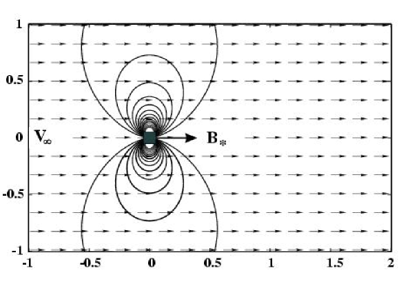
  Fig. 1.—: Geometry of the MHD simulation model. The solid lines are magnetic field lines which are constant values of the flux function, $\Psi(r,z)=$const. The $\Psi$ values shown are equally spaced between $\Psi_{min}=2\times 10^{-5}$ and $\Psi_{max}=10^{-4}$ in dimensionless units discussed in §3.

Recently it has been emphasized that some neutron stars, termed magnetars, may have anomalously strong magnetic fields at their origin $B\sim 10^{14}-10^{16}~{}{\rm G}$ (Duncan & Thompson 1992; Thompson & Duncan 1995 (hereafter TD95); Thompson & Duncan 1996). Magnetars pass through their pulsar stage much faster than classical pulsars, in $\sim 10^{4}$ years (TD95). Observations of soft gamma-ray repeaters (SGRs) and long-period pulsars in supernova remnants, especially young supernova remnants (Vasisht & Gotthelf 1997) support the idea that these objects are magnetars (Kulkarni & Frail 1993; Kouveliotou et al. 1994). The estimated birthrate of SGRs is $\sim 10\%$ of ordinary pulsars (Kulkarni & Frail 1993; Kouveliotou et al. 1994, 1999). Thus magnetars may constitute a non-negligible percentage of IONS.

MIONS and magnetars typically move supersonically through the ISM and have extended magnetospheres. Two main regimes are possible: In the first, the Alfvén radius $R_{A}$ is much smaller than gravitational accretion radius $R_{acc}$, so that matter is gravitationally attracted by the star and direct accretion to a star is possible (e.g. Hoyle and Lyttleton 1939; Bondi 1952; Lamb, Pethick, & Pines 1973; Bisnovatyi-Kogan & Pogorelov 1997). In the second regime, the magnetic standoff distance or Alfvén radius $R_{A}$ is larger than accretion radius and the magnetosphere interacts with the ISM without gravitational focusing. This case we term the “magnetic plow” regime (this corresponds to “georotator” regime in Lipunov, 1992). This is the regime for fast moving MIONS and magnetars. Neither of these regimes was investigated numerically in application to magnetized star propagation through the ISM. Most of simulations of this type were done to model the interaction of the Earth’s magnetosphere with the Solar wind (e.g., Nishida, Baker & Cowley 1998), where parameters of the problem were fixed by the Solar wind and Earth’s magnetic field.

In this paper we investigate the supersonic motion of magnetized stars through the ISM where a wide range of physical parameters is possible. We investigate the physical process of interaction of magnetospheres with the ISM and estimate the possible observational consequences of such interaction. In §2 we estimate the important physical parameters, and in §3 we describe the numerical model. In §4 we summarize results of simulations for $R_{A}\mathrel{\hbox{\hbox to0.0pt{\hbox{\lower 4.0pt\hbox{$\sim$}}\hss}\hbox{$<$}}}R_{acc}$ and for a small Mach number, ${\cal M}=3$. In §5 we discuss results of simulations in the “magnetic plow” regime. In §6 we discuss possible observational consequences of our results. In §7 we give a brief summary.

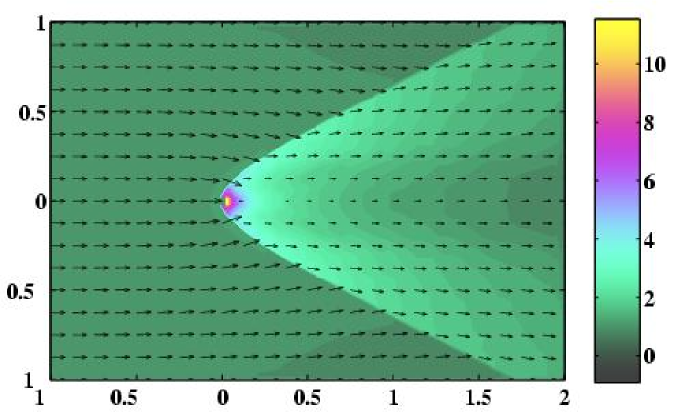
  Fig. 2.—: Results of hydro simulations of accretion to a non-magnetized star at Mach number ${\cal M}=3$. The background and contours represent density. Arrows represent velocity vectors.

2 Physical Model

After the radio pulsar stage, neutron stars are still strongly magnetized and rotating objects. This work treats the motion of a non-rotating magnetized star through the interstellar medium. Treatment of the motion of a rotating star through the ISM is discussed by Romanova et al. (2001).

A non-magnetized star moving through the ISM captures matter gravitationally from the accretion radius (e.g. Shapiro & Teukolsky 1983),

$$R_{acc}={2GM\over c_{s}^{2}+v^{2}}\approx 9.4\times 10^{11}{M_{1.4}\over v_{200}^{2}}~{}{\rm cm}~{},$$

where $v_{200}\equiv v/(200~{}{\rm km/s})$ is the normalized velocity of the star, $c_{s}$ the sound speed of the undisturbed ISM, and $M_{1.4}\equiv M/(1.4M_{\odot})$ is the normalized mass of the star. The mass accretion rate at high Mach numbers ${\cal M}\equiv v/c_{s}>>1$ was derived by Hoyle and Lyttleton (1939),

$$\dot{M}_{HL}=4\pi(GM)^{2}{\rho\over v^{3}}\approx 9.3\times 10^{7}{n\over v_{200}^{3}}M_{1.4}^{2}~{}{\rm\frac{g}{s}}~{},$$

where $\rho$ is the mass-density of the ISM and $n=n/{1~{}{\rm cm}^{-3}}$ is the normalized number density. For arbitrary ${\cal M}$ a general formulae was proposed by Bondi (1952),

$$\dot{M}_{BHL}=\pi R_{acc}^{2}\rho v=4\pi\alpha(GM)^{2}{\rho\over(v^{2}+c_{s}^{2})^{3/2}}~{},$$

where the coefficient $\alpha$ is of order unity (e.g., Bondi proposed $\alpha=1/2$, see also Ruffert 1994a,b; Pogorelov, Ohsugi, & Matsuda 2000).

For the case of a moving magnetized star, the standoff distance where the inflowing ISM is stopped by the star’s $B-$field is referred to as the Alfvén radius $R_{A}$. For a relatively weak stellar magnetic field $R_{A}\ll R_{acc}$, and in this limit of “gravitational accretion” denote the Alfvén radius as $R_{Ag}$. The accretion flow becomes spherically symmetric inside $R_{acc}$, and one finds

$$R_{Ag}=\bigg{(}\frac{B_{*}^{2}R_{*}^{6}}{\sqrt{2GM}\dot{M}}\bigg{)}^{2/7}~{}{\rm cm}~{},$$

(e.g., Lamb, et al. 1973, Lipunov 1992), where $B_{*}$ is the magnetic field at the surface of the star of radius $R_{*}$ and $\dot{M}$ is the accretion rate. If a magnetized star accretes matter with the same rate as a non-magnetized star, $\dot{M}=\dot{M}_{BHL}$, then the Alfvén radius is

$$R_{Ag}\approx 1.2\times 10^{11}\frac{B_{12}^{4/7}R_{6}^{12/7}v_{200}^{6/7}}{M_{1.4}^{5/7}n^{2/7}}~{}{\rm cm}~{},$$

which is about $R_{acc}/8$ for the adopted reference parameters. Here, $B_{12}\equiv B_{*}/10^{12}$G and $R_{6}\equiv R_{*}/10^{6}$cm.

However, there is reason to believe that a magnetized star accretes matter at a lower rate than a non-magnetized star for the same $v,~{}c_{s},$ and $M$. Our study of spherical Bondi accretion has shown that the magnetized star accretes at a lower rate than the same non-magnetized star (Toropin et al. 1999, hereafter T99). The magnetosphere acts as an obstacle for the flow, thus decreasing the rate of spherical accretion compared to the Bondi rate $\dot{M}_{B}=4\pi\alpha(GM)^{2}\rho/c_{s}^{3}$. Equations (28) and (32) of T99 correspond to the approximate dependence

$$\frac{\dot{M}}{\dot{M}_{B}}\approx\bigg{(}\frac{R_{*}}{R_{Ag}^{th}}\bigg{)}^{7/4}~{},$$

for $R_{Ag}^{th}/R_{*}$ in the range $1-10$, where $R_{Ag}^{th}$ is given by equation (4) with $\dot{M}=\dot{M}_{B}$. Thus, for a larger $R_{Ag}^{th}$, $\dot{M}$ is smaller and the actual Alfvén radius given by equation (4) is larger.

Equation (6) was deduced from simulations at small values of $R_{Ag}/R_{*}$ and therefore it cannot be reliably extrapolated to very large values of this ratio. Instead we can write in general $\dot{M}={\cal K}\dot{M}_{B}$ where ${\cal K}\leq 1.$ Then we find that the actual Alfvén radius is $\tilde{R}_{Ag}=R_{Ag}^{th}{\cal K}^{-2/7}$. The two radii, $R_{acc}$ and $\tilde{R}_{Ag}$ are equal at ${\cal K}\approx 10^{-3}$ for our reference parameters. It is not known whether accretion can be so strongly inhibited at such small values of ${\cal K}$.

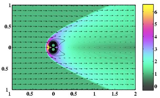
  Fig. 3.—: Results of simulations of accretion to a magnetized star with magnetic field $B_{*}=3.5$ at Mach number ${\cal M}=3$. Poloidal magnetic field lines and velocity vectors $\bf v$ are shown. The background represents density. The thick line represents the Alfvén surface.

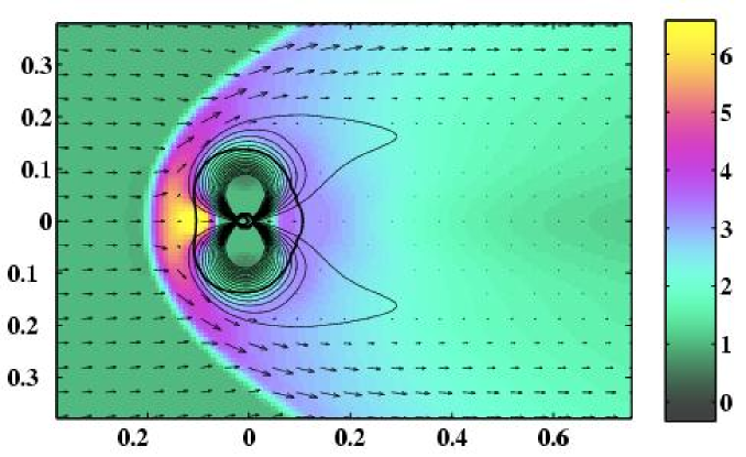
  Fig. 4.—: Same case as Figure 3, but the inner region is shown at higher resolution. Arrows show matter flux vectors $\rho{\bf v}$. The thick line represents the Alfvén surface.

Magnetars have significantly stronger magnetic fields than typical radio pulsars, and consequently most of them are in the “magnetic plow” regime. Comparison of equations (1) and (5) shows that $R_{acc}\leq\tilde{R}_{A}$ if

$$B_{*}\geq 3.7\times 10^{13}\frac{{\cal K}^{1/2}M_{1.4}^{3}n^{1/2}}{R_{6}^{3}v_{200}^{5}}~{}{\rm G}~{}.$$

Thus, even for ${\cal K}=1$ and $v\approx 200~{}{\rm km/s}$, magnetars are in the magnetic plow regime.

In the “magnetic plow” regime, the Alfvén radius $R_{Ap}$ follows from the balance of the magnetic pressure of the star $B^{2}/4\pi=B_{*}^{2}(R_{*}/R)^{6}$ against the ram pressure of the ISM which is $\rho v^{2}$ for Mach numbers ${\cal M}\gg 1$. Thus

$$R_{Ap}=R_{*}\bigg{(}\frac{B_{*}^{2}}{4\pi\rho v^{2}}\bigg{)}^{1/6}\approx 2.2\times 10^{11}R_{6}\bigg{(}\frac{B_{12}^{2}}{4\pi nv_{200}^{2}}\bigg{)}^{1/6}~{}{\rm cm}~{}.$$

The magnetic field strength at this distance from the star is

$$B_{A}=(4\pi\rho)^{1/2}v\approx 9.2\times 10^{-5}n^{1/2}v_{200}~{}{\rm G}~{}.$$

At the boundary between the gravitational and magnetic plow regimes, equations (1), (4), and (8) coincide. We mention here the important influence of rotation of the star. Due to the rotation the magnetic field decreases with distance $\propto 1/r$ at large distances rather than $\propto 1/r^{3}$ so that the Alfvén radius is much larger than one described by equation (8) (Romanova et al. 2001).

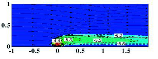
  Fig. 5.—: Same case as Figure 3, but the streamlines of matter flux $\rho{\bf v}$ are shown. Background and dashed lines represent logarithm of magnetic flux which is equally spaced between $\log_{10}\Psi=-6$ and $\log_{10}\Psi=-4$. The minimum value of $\Psi$ is smaller than that in Figure 3. Numbers show the value of logarithm of $\Psi$.

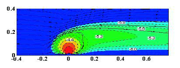
  Fig. 6.—: Same case as Figure 5, but the inner region is shown at higher resolution.

The velocity distribution of MIONS and magnetars is unknown, but it is expected to be similar to that of radio pulsars. Pulsars have a wide range of velocities, $10~{}{\rm km/s}\leq{\bar{v}}\leq 1500~{}{\rm km/s}$, with the peak of the distribution at $\bar{v}\approx 175~{}{\rm km/s}$ (Cordes & Chernoff 1998). Some authors give a smaller value, ${\bar{v}}\approx 100~{}{\rm km/s}$ (Narayan & Ostriker 1990) while others give larger values, ${\bar{v}}\approx 250-300~{}{\rm km/s}$ (Hansen & Phinney 1997), ${\bar{v}}\approx 500~{}{\rm km/s}$ (Popov et al. 2000). For temperatures of the ISM, $T\approx 10^{4}~{}{\rm K}$, the sound speed of gas is $c_{s}\approx\sqrt{\gamma k_{B}T/\bar{m}}\approx 11.7~{}{\rm km/{s}}$, where $\bar{m}\approx m_{p}$ is the mean particle mass, $k_{B}$ is Boltzmann’s constant, and $\gamma$ is the usual specific heat ratio. Thus, the Mach number of radio pulsars is in the range ${\cal M}=v/c_{s}\sim 1-150$ with most pulsars having ${\cal M}\sim 10-50$. The accretion radius $R_{acc}$ depends strongly on the velocity of the star $v$, which may change the ratio between $R_{acc}$ and $R_{A}$ and correspondingly the regime of accretion. For example, very fast MIONS with $v\sim 1000~{}{\rm km/s}$ have much smaller accretion radii than slow ones, and may have $R_{A}>>R_{acc}$ for wide range of magnetic fields.

It is clear from the range of surface magnetic fields of MIONS and magnetars and the range of their velocities that different regimes are possible: (1) The regime of gravitational accretion, $R_{acc}>>R_{A}$; (2) The intermediate regime, $R_{acc}\sim R_{A}$; and (3) The “magnetic plow” regime, $R_{acc}<<R_{A}$. In this paper, we present results for regimes (2) and (3), which are characterized by formation of extended magnetotails. Regime (1) will be investigated in a future work. Below, we present numerical model and results of simulations, and return to discuss physical model further in §6, where the possible observational consequences are considered.

3 Numerical Model

To investigate the interaction of a magnetized star with the ISM we use an axisymmetric resistive MHD code and arrange dipole so that its axis is aligned with the matter flow (see Figure 1). The code uses a total variation diminishing (TVD) method (Savelyev et al. 1996; Zhukov et al. 1993). The code was used earlier for a study of spherical Bondi accretion to a star with dipole magnetic field (T99).

We used a cylindrical coordinate system $\left(r,\phi,z\right)$ with its origin at the star’s center. The $z$-axis is parallel to the velocity of the ISM at large distances ${\bf v}_{\infty}$. The dipole magnetic moment of the star ¯ is parallel or antiparallel to the $z-$axis. Axisymmetry is assumed so that ${\partial}/{\partial\phi}=0$ for all scalar variables. We solve for the vector potential ${\bf A}$ so that the magnetic field ${\bf B}={\bf\nabla}\times{\bf A}$ automatically satisfies ${\bf\nabla}\cdot{\bf B}=0$.

The flow is described by the resistive MHD equations,

$${\partial\rho\over\partial t}+{\bf\nabla}{\bf\cdot}\left(\rho~{}{\bf v}\right)=0~{},$$

$$\rho\left(\frac{\partial}{\partial t}+\left({\bf v}{\bf\cdot}{\bf\nabla}\right)\right){\bf v}=-{\bf\nabla}p+{1\over c}{\bf J\times B}+{\bf F}^{g}~{},$$

$$\frac{\partial{\bf B}}{\partial t}={\bf\nabla}{\bf\times}\left({\bf v}{\bf\times}{\bf B}\right)+\frac{c^{2}}{4\pi\sigma}\nabla^{2}{\bf B}~{},$$

$$\frac{\partial(\rho\varepsilon)}{\partial t}+{\bf\nabla}\cdot\left(\rho\varepsilon{\bf v}\right)=-p\left({\bf\nabla}{\bf\cdot}{\bf v}\right)+{1\over\sigma}{\bf J}^{2}~{}.$$

The variables have their usual meanings. The equation of state is $p=\left(\gamma-1\right)\rho\varepsilon$, with $\gamma$ the specific heat ratio. In the simulations presented here $\gamma=5/3$. The equations incorporate Ohm’s law ${\bf J}=\sigma({\bf E}+{\bf v}\times{\bf B}/c)$, where $\sigma$ is the electrical conductivity. The corresponding magnetic diffusivity $\eta_{m}\equiv c^{2}\!/(4\pi\sigma)$ is taken to be a constant.

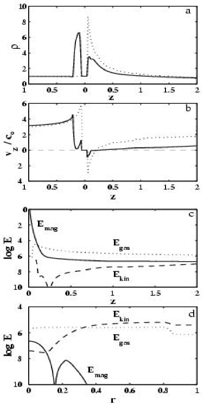
  Fig. 7.—: Panel (a) shows the density and panel (b) the velocity variation along the $z-$ axis. Panel (c) shows the energy-density variation along the $z-$ axis, and panel (d) shows its variation with $r$ at $z=1$. Here, $E_{mag}-$is the magnetic energy-density, $E_{kin}-$ is the kinetic energy-density, and $E_{gas}$ is the thermal energy-density. For the case shown, $B_{*}=3.5$ and ${\cal M}=3$. Dotted lines on panels (a,b) correspond to hydrodynamic simulations.

The simulations were done inside a “cylindrical box,” $(Z_{min}\leq z\leq Z_{max},0\leq r\leq R_{max})$. A uniform $(r,z)$ mesh was used with size $N_{R}\times N_{Z}.$ The magnetized star was represented by a small cylindrical box with dimensions $R_{*}<<R_{max}$ and $|Z_{*}|<<Z_{max}$, which constitutes the “numerical star.” In equation (11) the gravitational force is due to the star, ${\bf F}^{g}=-GM\rho{\bf R}/\!R^{3}$. The gravitational force was smoothed for distances inside the region $r=|z|=0.25R_{*}$ which does not influence the computational results outside of the numerical star.

A point dipole magnetic field ${\bf B}=[3{\bf R}\left({{\hbox{\tenbg\char 22\relax}}}\cdot{\bf R}\right)-R^{2}{\hbox{\tenbg\char 22\relax}}]/{R^{5}}$ with vector-potential ${\bf A}={{{\hbox{\tenbg\char 22\relax}}}\times{\bf R}}/{R^{3}}$ was arranged inside numerical star at the radii: $r>0.25R_{*}$. This dipole field differs from that used in T99 where a small but finite size “current” disk was used to produce the dipole field. A similar model of the field was used by Hayashi et al. (1996), Miller & Stone (1997), Goodson et al. (1997).

The vector potential was fixed inside the numerical star and at its surface during the simulations. These conditions follow from the ${\bf E}$ and ${\bf B}$ boundary conditions on the surface of the perfectly conducting star and protect the magnetic field against numerical decay (T99). The hydrodynamic variables $\rho,$ $v_{r},$ $v_{z},$ and $\varepsilon$ were fixed at the surface of the numerical star. These conditions are similar to the standard “vacuum” conditions adopted in hydrodynamic simulations (e.g., Ruffert 1994a,b). However, the vacuum is not made too strong because of the difficulty of handling low densities in MHD simulations. We discuss the boundary conditions on the numerical star further in §4.1. We tested the influence of the numerical star shape on our simulation results. Namely, we created an approximation of a sphere on rectangular grid and compared it with the cylindrical star and observed that the difference in the shapes has an insignificant influence on our results.

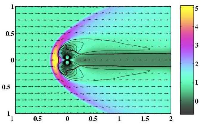
  Fig. 8.—: Results of simulations of motion of a magnetized star with magnetic field $B_{*}=14$ through the ISM with Mach number ${\cal M}=3$. Magnetic field lines and velocity vectors are shown. The background represents the density. The thick line indicates the Alfvén surface.

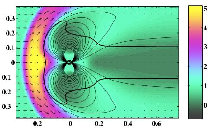
  Fig. 9.—: Same run as Figure 8, but the inner region is shown at higher resolution. Arrows show matter flux vectors $\rho\bf v$. The thick line represents the Alfvén surface.

We put the MHD equations in dimensionless form using the following scalings: The characteristic length is taken to be the Bondi radius, $R_{B}={GM}/c_{s\infty}^{2}$, where $c_{s\infty}$ is the sound speed in the undisturbed ISM. Temperature is measured in units of $T_{\infty}$, and density in units of $\rho_{\infty}$. The magnetic field is measured in units of the reference magnetic field $B_{0}$. A reference speed is the Alfvén velocity corresponding to a reference magnetic field $B_{0}$ and density $\rho_{\infty}$, $v_{0}\equiv{B_{0}}/\sqrt{4\pi\rho_{\infty}}$. Time is measured in units of $t_{0}=(Z_{max}-Z_{min})/v_{\infty}$, which is the crossing time of the computational region in the absence of a star. After reduction to dimensionless form, the MHD equations (10) - (13) involve three dimensionless parameters,

$$\beta\equiv\frac{8\pi p_{\infty}}{B_{0}^{2}}~{},\quad\quad g\equiv\frac{GM}{R_{B}v_{0}^{2}}=\frac{1}{2}\gamma\beta~{},$$

$$\tilde{\eta}_{m}\equiv{\eta_{m}\over R_{B}v_{0}}={1\over Re_{m}}{~{},}$$

where $\tilde{\eta}_{m}$ is the dimensionless magnetic diffusivity, and $Re_{m}$ is the magnetic Reynolds number. Note that the first two parameters are dependent because of our choice of the length scale $R_{B}$.

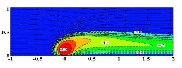
  Fig. 10.—: Same case as Figure 8, but the streamlines (solid lines) of matter flux $\rho{\bf v}$ are shown. The background represent logarithm of magnetic flux which is equally spaced between $\log_{10}\Psi=-6$ and $\log_{10}\Psi=-4$. The numbers indicate the logarithm of $\Psi$.

The external boundaries of the computational region were treated as follows. Supersonic inflow with Mach number ${\cal M}$ was specified at the upstream boundary $(z=Z_{min},0\leq r\leq R_{max})$. At the downstream boundary $(z=Z_{max},0\leq r\leq R_{max})$, a “free boundary” condition was applied, $\partial/\partial{\bf n}=0$. Inflow of matter from this boundary into the computational region was forbidden. At the cylindrical boundary $(Z_{min}\leq z\leq Z_{max},r=R_{max}$, we used the free boundary conditions and in some cases forbid inflow to the computational region. We observed that the result is very similar in both cases. We checked the influence of external boundary conditions by performing test simulations at different sizes of the computational region.

The size of the computational region for most of the simulations was $R_{max}=2R_{B}=2$, $Z_{min}=-R_{max}=-2$, and $Z_{max}=2R_{max}=4$. The grid $N_{R}\times N_{Z}$ was $257\times 769$ in most of cases. The radius of the numerical star was $R_{*}=0.05{}R_{B}=0.05$ in most cases, but test runs were also done for $R_{*}=0.02$. A number of different values of $R_{*}$ were investigated in the purely hydrodynamic simulations (see §4.1).

For most of our simulation runs $\beta=10^{-6}$. Therefore, our reference magnetic field $B_{0}=\sqrt{8\pi p_{\infty}/\beta}$ is also fixed since $p_{\infty}$ is fixed. Thus a useful measure of the strength of the magnetic field is the ratio of the maximum value of the $z-$component of the field at the point $r=0.25R_{*}$ and $z=0$ to $B_{0}$. We denote this dimensionless field as $B_{*}$. We performed simulations for a range of values of $B_{*}$. The magnetic diffusivity was taken to be $\tilde{\eta}_{m}=10^{-6}$ in most of runs, but the dependence of our solutions on $\tilde{\eta}_{m}$ is discussed in §5.2.

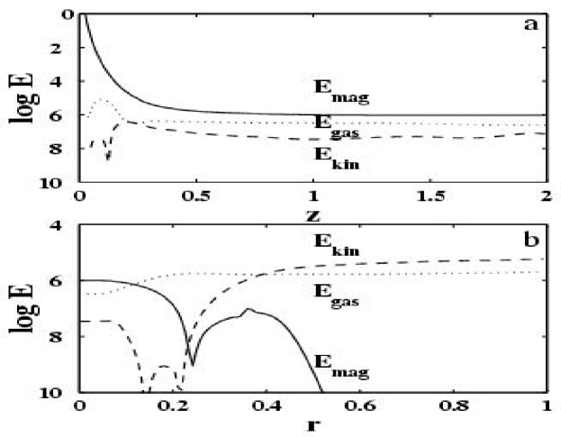
  Fig. 11.—: Panel (a) shows the energy-density variation along the tail. Panel (b) shows the variation across the tail at $z=1$. Both panels are for $B_{*}=14$, ${\cal M}=3$. Here, $E_{mag}$ is the magnetic energy-density, $E_{kin}-$ the kinetic energy-density, and $E_{gas}$ the thermal energy-density.

Initially, at $t=0$ the magnetic field of the star is a dipole field. The density and flow velocity are homogeneous in the simulation region: $\rho=\rho_{\infty}$ and $v=v_{\infty}$ (see Figure 1). We investigate subsequent evolution and follow the evolution as long as it is needed to reach stationarity or quasi-stationarity. This is typically several dynamical time-scales.

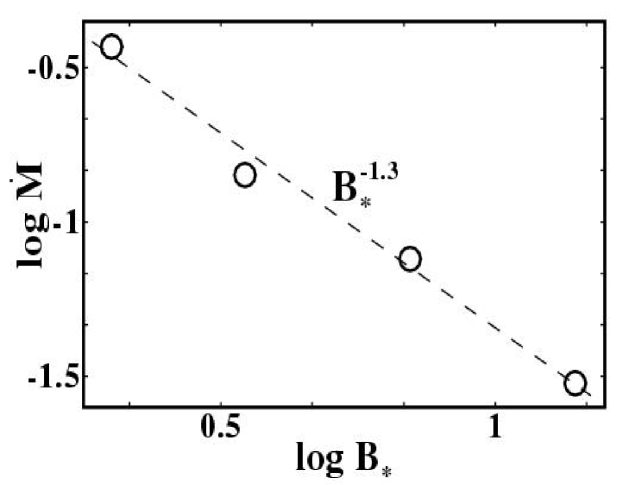
  Fig. 12.—: Dependence of the accretion rate to a star on the surface magnetic field $B_{*}$ for a star moving at Mach number ${\cal M}=3$.

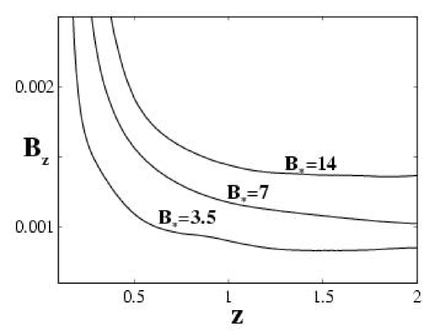
  Fig. 13.—: Variation of the magnetic field along the tail at $r=0$ for $z\mathrel{\hbox{\hbox to0.0pt{\hbox{\lower 4.0pt\hbox{$\sim$}}\hss}\hbox{$>$}}}0.1$, ${\cal M}=3$ and different values of the magnetic field $B_{*}$ at the star’s surface.

4 Accretion for $R_{A}\sim R_{acc}$ and ${\cal M}=3$

In this section we take the Mach number to be relatively small, ${\cal M}=3$, so that the accretion radius $R_{acc}$ is of the order of magnitude of the Alfvén radius $R_{A}$.

4.1 Hydrodynamic Simulations

First, for reference, we did hydrodynamic simulations of the BHL accretion to a non-magnetized star for Mach number ${\cal M}=3$. We verified that the nature of the flow is close to that described by earlier investigators of hydrodynamic BHL accretion (e.g., Matsuda et al. 1991; Ruffert 1994b). Namely, incoming matter forms a conical shock wave around the star. Figure 2 shows the main features of the flow at a late time $t=6.7t_{0}$ when the flow is stationary. The opening angle of the shock wave at large distances from the star relative to the $z-$axis is predicted to be $\theta={\rm arcsin}(1/{\cal M})$, which is $\theta=19.5^{\circ}$ for ${\cal M}=3$. Our simulations give $\theta\approx 25^{\circ}$, which is larger than predicted. However, when we performed the simulations in an enlarged region, $R_{max}=2$, $Z_{min}=-2$, $Z_{max}=4$, on a grid $N_{R}\times N_{Z}=257\times 769$, we obtained $\theta\approx 23^{\circ}$ which is close to the theoretical value and similar to the value obtained by Ruffert (1994b).

We calculated the accretion rate $\dot{M}$ to the numerical star and got a value $\dot{M}\approx 0.5\dot{M}_{BHL}$. We performed simulations using a smaller numerical star $R_{*}=0.02$ and got a slightly smaller value $\dot{M}\approx 0.4\dot{M}_{BHL}$. This behavior agrees with Ruffert’s results on the dependence of $\dot{M}$ on numerical star size for the sizes used, $R_{*}=0.25R_{acc}$ and $R_{*}=0.1R_{acc}$ (Ruffert 1994 a,b). This size dependence becomes negligibly small for $R_{*}<0.1R_{acc}$. In our simulations of accretion to magnetized stars we take the larger value $R_{*}=0.05=0.25R_{acc}$, because it gives better resolution of the magnetic field near the star.

We compared simulations in the region ($R_{max}=2R_{B}$, $Z_{max}=4R_{B}$) with simulations in twice as smaller region. This gave only a $\sim 5\%$ decrease of accretion rate, which means that our standard region $R_{max}=2R_{B}=2$ is sufficiently large to accumulate matter from the far distances, though simulations in smaller regions will be also sufficient. Usually, a low pressure is arranged inside the numerical star (e.g., Ruffert 1994 a,b). However, it is impossible to perform MHD simulations with very low pressure and density inside the numerical star. In our MHD simulations we have $\rho=\rho_{0}=1$ inside the numerical star. To test the influence of this value, we performed simulations with lower densities inside numerical star, $\rho_{acc}=10^{-2}\rho_{0}$ and $10^{-3}\rho_{0}$ We observed, that this changed only slightly the accretion rate (at the level $<5\%$). This is connected with the fact that the matter density which accumulates around the star before accretion is much larger than $\rho_{0}$, so that the difference $\Delta\rho=\rho-\rho_{0}$ is about the same for considered values of $\rho_{0}$.

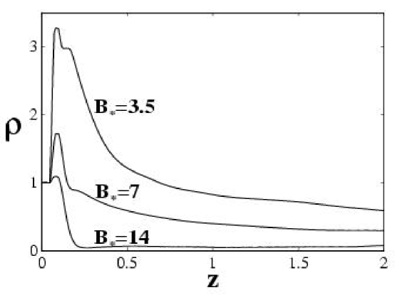
  Fig. 14.—: Axial distribution of density in the tail for ${\cal M}=3$ and different values of the magnetic field $B_{*}$.

4.2 Accretion to a Magnetized Star

Next, we investigated propagation of a magnetized star through the ISM. Simulations were performed for a number of values of the magnetic field $B_{*}$. We show results for two cases: for a relatively weak magnetic field, $B_{*}=3.5$ (where $R_{A}<R_{acc}$); and for a strong magnetic field, $B_{*}=14$ (where $R_{A}>R_{acc}$).

Figure 3 shows the main features of the flow for a star with $B_{*}=3.5$ at time $t=5t_{0}$ when the flow is stationary. One can see that the magnetic field of the star acts as an obstacle for the flow and a conical shock wave forms as in the hydrodynamic case with similar angle $\theta$ as expected since the Mach numbers are the same. Magnetic field lines (with flux values the same as in Figure 1) are slightly stretched by the flow, but they remain closed. Figure 4 shows the inner region of the flow in greater detail. The bold line represents the Alfvén surface, where the matter energy-density $\rho(\varepsilon+v^{2}\!/\!2)$ is equal to the magnetic energy-density $B^{2}/(8\pi)$. The radius of Alfvén surface in $z-$ direction downstream at $r=0$ is $R_{A}\approx 0.1$, and in $r-$ direction at $z=0$ is $R_{A}\approx 0.14$ which is smaller than accretion radius $R_{acc}\approx 0.2$. Thus, some gravitational focusing is expected and indeed we observe density enhancement around the star. Figures 5 and 6 show the distribution of magnetic flux with the lower limit ${\rm log}_{10}\Psi_{min}=-6$ compared to that shown in Figures 3 and 4 where ${\rm log}_{10}\Psi_{min}\approx-5.3$. Thus the apparent truncation of the magnetosphere in Figures 3 and 4 was connected with choice of minimum plotted magnetic flux. Streamlines of matter flow $\rho{\bf v}$ shown in Figures 5 and 6 reveal that matter from radii $r<0.1R_{acc}$, accretes to the star, while the rest of matter flies away. Compared with the non-magnetized case, the magnetic field acts as an obstacle for the flow, and most of the inflowing matter is kept away from the star.

The matter density is strongly enhanced in the shock wave, but gradually decreases as it approaches the surface of the star where it accretes (Figure 7a). Behind the star (for $0<z<0.4$) there is also an accumulation of matter connected with gravitational focusing by a star. Note, that in the case of hydrodynamic accretion, the density jump in front of the star (at $z<0$) is much smaller, while behind the star (at $z>0$) it is much larger. The velocity $v_{z}$ (panel b) decreases sharply in the shock wave to small subsonic values, but later increases again in the polar column. Behind the star the velocity is negative in the small region $0.05<z<0.1$, where accretion occurs. The density and velocity jumps in front of the star do not satisfy the standard Rankine-Hugoniot conditions, because the shock wave is “attached” to the magnetosphere. Matter cannot move freely after passage through the shock wave, and extra matter accumulation occurs in the shock.

From panels (a) and (b) of Figure 7 it is clear that the rate of accretion is smaller in the case of a magnetized star compared to a non-magnetized star. We observed, that the accretion rate to a magnetized star for $B_{*}=3.5$ is about $3$ times smaller than that to a non-magnetized star. The variations of the of energy-densities along and across the tail (Figure 7c, d) shows that magnetic energy-density dominates only in a small region around the star.

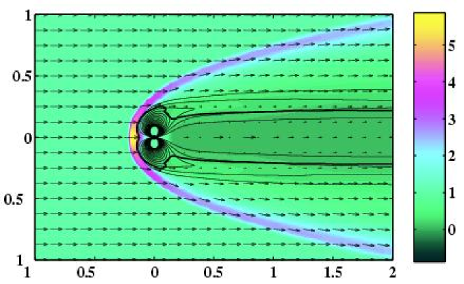
  Fig. 15.—: Results of simulations for ${\cal M}=10$ and $B_{*}=14$.

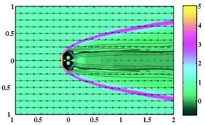
  Fig. 16.—: Results of simulations for ${\cal M}=30$ and $B_{*}=14$.

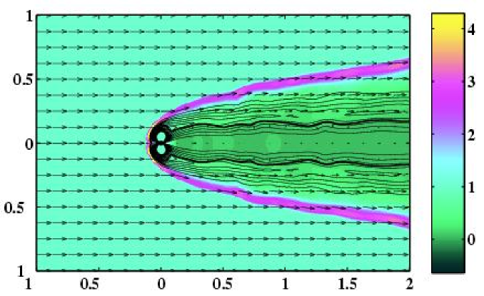
  Fig. 17.—: Results of simulations for ${\cal M}=50$ and $B_{*}=14$.

In case of a stronger magnetic field, $B_{*}=14$, larger magnetic flux is stretched downwind (see Figure 8). Gravitational focusing is still important and density enhancement is observed around the star, but it is much smaller, than in case of weaker magnetic field $B_{*}=3.5$. Now, the Alfvén surface has elongated structure and extends all along the $z-$axis, so that the magnetic energy-density predominates in the tail (see Figure 8).

The magnetosphere around the star is larger than in the case $B_{*}=3.5$, and the Alfvén radius in $r$ direction is $R_{A}\approx 0.26$, which is larger than accretion radius $R_{acc}=0.2$ (Figure 9). Now, all incoming matter goes around the magnetosphere and flies away. Streamlines of the flow (Figure 10) show, that no matter goes from the front and accretes to the back side of the star. A small flux of matter coming from $r<<R_{acc}$, accretes directly to the upwind pole of the star.

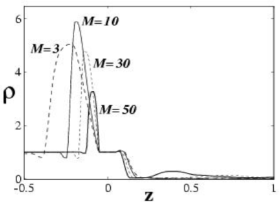
  Fig. 18.—: Axial density variations at different Mach numbers and $B_{*}=14$.

Figure 11a shows, that at $B_{*}=14$, compared to $B_{*}=3.5$, magnetic energy-density predominates in the tail in the region of equatorial plane. Figure 11b and also Figure 8 and 9, show that in $r-$ direction magnetic energy-density dominates in the tube with radius $r\approx 0.11$.

We performed additional simulations for magnetic fields strengths $B_{*}=2$, $7$, and $11$, and derived the dependence of the accretion rate on the magnetic field strength $B_{*}$ for all cases. We observed that accretion rate strongly decreases with increasing magnetic field (see Figure 12) as $\dot{M}\sim B_{*}^{-1.3\pm 0.05}$. This dependence reflects the fact that a stronger magnetic field of the star deflects the incoming ISM flow more efficiently than weaker magnetic field.

Figure 13 shows axial variation of $B_{z}$ for different values of $B_{*}$. In all cases the magnetic field decreases very gradually with $z$: $B_{z}\sim z^{-0.15}$. The decrease is partially connected with gradual radial expansion of the magnetosphere, and partially with the reconnection of magnetic field lines in the tail. In the actual flow, the magnetic diffusivity is expected to be much smaller than that in the code. This acts to decrease the reconnection rate and increase the length of the tail. Note that the tail of Earth’s magnetosphere extends to more than a hundred of Earth radii (e.g., Nishida et al. 1998). The value of the field in the tail is larger for larger values of $B_{*}$. Even for $B_{*}=3.5$ the magnetic field stretches a long distance downwind from the star. The Alfvén surface in this case is small not only because the magnetic field is weak, but also because matter energy-density is high. At magnetic field strengths $B_{*}<2-3$, however, stretching of magnetic field to the tail becomes suppressed.

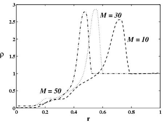
  Fig. 19.—: Radial density variations at $z=1$ for different Mach numbers and $B_{*}=14$.

For $B_{*}>7$ ($R_{A}\mathrel{\hbox{\hbox to0.0pt{\hbox{\lower 4.0pt\hbox{$\sim$}}\hss}\hbox{$>$}}}R_{acc}$), the density in the magnetotail is lower than that in the incoming flow $\rho_{0}$ and it decreases at higher $B_{*}$ (see Figure 14). Thus, one can expect hollow magnetic tails in the case of strongly magnetized stars. This is connected with the fact, that magnetosphere is an obstacle for the flow and the tail represents the rarefaction region which usually forms behind an obstacle in a supersonic flow (e.g. Landau & Lifshitz 1960). Furthermore, external matter penetrates only slowly across the magnetotail, because the magnetic diffusion time-scale across the tail is long compared with the transit time of the matter in the $z-$direction.

5 “Magnetic Plow” Regime ($R_{A}>>R_{acc}$)

In this section we investigate interaction of magnetosphere with the ISM in “magnetic plow” regime, where the Alfvén radius $R_{A}$ is much larger than accretion radius $R_{acc}$. In this limit gravitational focusing is unimportant and there is only direct interaction of the ISM with magnetosphere of the star. For Mach numbers larger than about ${\cal M}=3$ (for our set of parameters $B_{*}$), the flow is in the “magnetic plow” regime. In this section we investigate properties of magnetotails at different Mach numbers ($\S 5.1$) and different magnetic diffusivities ($\S 5.2$).

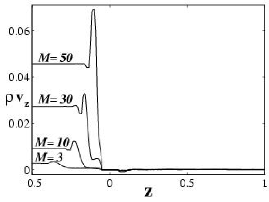
  Fig. 20.—: Axial variation of the matter flux $\rho v_{z}$ at different Mach numbers ${\cal M}$ and $B_{*}=14$.

5.1 Investigation of Magnetotails at Different Mach Numbers ${\cal M}$

In this subsection we fix the magnetic field to be $B_{*}=14$ and the diffusivity $\tilde{\eta}_{m}=10^{-6}$ and investigate flows at Mach numbers ${\cal M}=10$, ${\cal M}=30$ and ${\cal M}=50$. We observed, that at high Mach numbers ${\cal M}$, the sharp density enhancement is observed in the shock cone, while the rest of the tail have low density (see Figures 15, 16 & 17). At very high Mach number ${\cal M}=50$, some kind of instability appears in the tail which determines its wavy behavior (Figure 17). This instability may be connected with high velocity gradient across the tail. The Alfvén radius in the $r$ direction and in the upwind $z$ direction decreases at larger $\cal M$ (see also equation 8), because the flow strips deeper layers of magnetosphere. This also leads to higher magnetic field in the tail. Reconnection is observed as in case of lower Mach numbers. However, the reconnection region is further downwind from the star at higher $\cal M$.

The axial density variations for the three cases are shown at Figure 18. The case with low Mach number ${\cal M}=3$ is included for reference. One can see that in case ${\cal M}=10$ the density in front of the star increases to $\rho_{front}=(5-6)\rho_{0}$ and then decreases sharply closer to the surface of numerical star. At higher Mach numbers, the density peak is lower. The density behind the star, in the tail, is small $\rho_{tail}\sim(10^{-1}-10^{-2})\rho_{0}$. The density variation across the tail at $z=1$ is shown at Figure 19. It shows that an essential part of the tail is hollow. The matter flux $\rho{\bf v}$ is much higher for higher Mach numbers (Figure 20), owing to higher velocities. The instability observed at ${\cal M}=50$ may be the Kelvin-Helmholtz instability connected with the large gradient in the flow velocity.

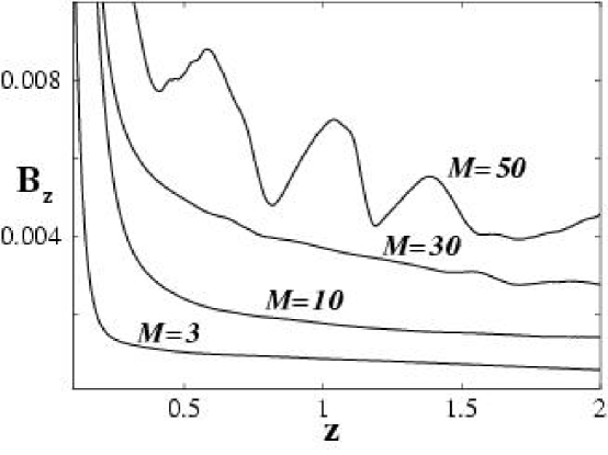
  Fig. 21.—: Variation of $B_{z}$ along the tail at $r=0$ for $B_{*}=14$ for different Mach numbers.

The axial magnetic field decreases slowly with distance behind the star, $B_{z}\sim z^{-0.2}$ (Figure 21). Thus, long tails form as in the case ${\cal M}=3$. The magnetic field in the tail is larger at larger Mach numbers.

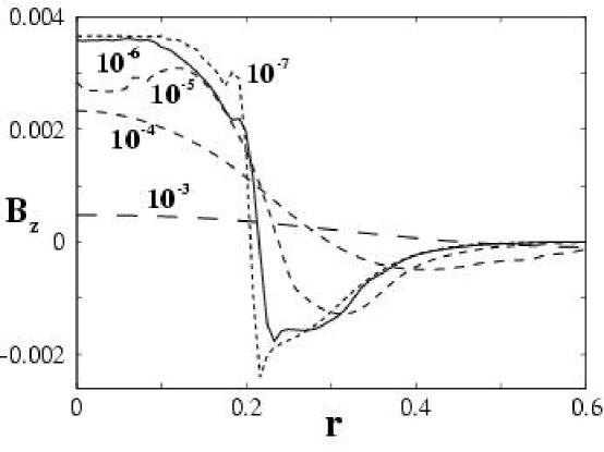
  Fig. 22.—: Variation of the magnetic field $B_{z}$ across the tail at $z=1$ for different values of the magnetic diffusivity $\tilde{\eta}_{m}$ for the case $B_{*}=14$ and ${\cal M}=30$.

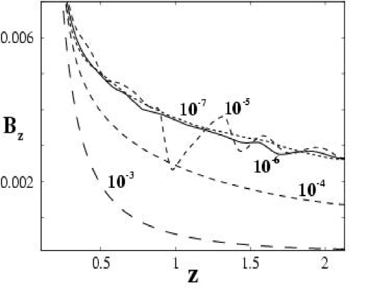
  Fig. 23.—: Variation of the magnetic field $B_{z}$ along the tail at $r=0$ for different values of the magnetic diffusivity $\tilde{\eta}_{m}$ for the case $B_{*}=14$ and ${\cal M}=30$.

5.2 Dependence of the Flow on Magnetic Diffusivity

The processes of accretion and reconnection of the magnetic field depend on the magnetic diffusivity $\tilde{\eta}_{m}$. The fact that our code explicitly includes $\tilde{\eta}_{m}$ allows us to investigate the dependence of the flows on the magnitude of this quantity. This is in contrast with ideal MHD codes where the magnetic diffusivity unavoidably arises from the finite numerical grid. To study the dependence on $\tilde{\eta}_{m}$, we fixed the magnetic field, $B_{*}=14$, and the Mach number, ${\cal M}=30$. We made simulation runs for a range of values between $\tilde{\eta}_{m}=10^{-3}$ and $10^{-8}$.

We observed that at lower magnetic diffusivity, the magnetic tail (the Alfvén surface) is wider in the $r$ direction. Figure 22 shows the variation of $B_{z}$ across the tail at $z=1$. One can see that at small $\tilde{\eta}_{m}=10^{-6}-10^{-7}$, regions with oppositely directed magnetic field are very close to each other, but do not reconnect. On the other hand, at large $\tilde{\eta}_{m}=10^{-3}-10^{-4}$, the magnetic field is much smaller, because it annihilates rapidly with distance behind the star. Furthermore, note that at large $\tilde{\eta}_{m}$, matter is partially decoupled from magnetic field and stretching of magnetic field is less efficient. Figure 23 shows the dependence of axial distribution of $B_{z}$ on $\tilde{\eta}_{m}$. One can see that at $\tilde{\eta}_{m}>10^{-5}$, the magnetic field decreases with $z$ very rapidly. Note, that at $\tilde{\eta}_{m}>3\times 10^{-7}$, numerical diffusivity predominates, and the calculated flows depend only weakly depends on $\tilde{\eta}_{m}$.

The observed behavior is determined by the magnetic Reynolds number,

$$Re_{m}\equiv{R~{}v\over\eta_{m}}={\tilde{R}~{}\tilde{v}\over\tilde{\eta}_{m}}~{},$$

where tilde-quantities are our dimensionless variables. For example, for ${\cal M}=3$ and $B_{*}=3.5$, in the upwind region of the flow, $Re_{m}\approx 400$ and most of the matter goes around the dipole and flies away or accretes to the downwind pole. Matter which goes to the downwind pole has smaller velocity and hence smaller $Re_{m}$. Also, when matter diffuses across the tail in the $r$ direction owing to gravitational force it has $v_{r}<<v_{z}$, and $Re_{m}\mathrel{\hbox{\hbox to0.0pt{\hbox{\lower 4.0pt\hbox{$\sim$}}\hss}\hbox{$<$}}}1$. However, the timescale of the flow in the $z-$ direction is much less than that in $r$ direction, so that most of the matter flies away. The main conclusion of this subsection is that the magnetotails lengthen as the diffusivity decreases. Comparison with the Earth’s magnetosphere (e.g., Nishida et al. 1998), shows that the actual diffusivity may be smaller than the smallest values used in our simulations.

6 Observational Consequences

The question arises, is it possible to observe either a bow shocks or the elongated magnetotails of magnetized old neutron stars or magnetars? In this section we estimate the powers released and other possible observational features of these objects.

6.1 Reconnection in the Tail

Our simulations show that the magnetic field in the tail reconnects. This phenomenon may lead to acceleration of particles and possible flares in the tail. The total magnetic energy stored in the tail can be estimated as

$$E_{tot}\approx{1\over 8\pi}\int\limits_{0}^{S}dz~{}\pi[R(z)]^{2}~{}[B(z)]^{2},$$

where $S$ is the length of the tail, $R(z)$ is the radius of the tail at $z$. The total magnetic flux in, say, the $+z$ direction along the tail,

$$\Phi_{mag}\approx B(z)\pi[R(z)]^{2}\approx B_{A}\pi R_{A}^{2}~{},$$

is constant in the absence of reconnection. Therefore, if the tail cross-section expands with distance $z$, then the magnetic field decreases as $B(z)=B_{A}(R_{A}/R(z))^{2}$. The values $R_{A}$ and $B_{A}$ we derived earlier [see equations (8) and (9)]. We observed that at high Mach numbers, the magnetotail expands in the $r$ direction very gradually. To estimate the total magnetic energy in a tail of length $S$, we suppose that the tail does not expand, ($R_{tail}\approx R_{A}$) thus

$$E_{tot}\approx{1\over 8\pi}{B_{A}^{2}}\pi R_{A}^{2}S\sim 10^{27}B_{12}n^{1/2}v_{200}~{}S_{100}~{}{\rm erg}~{},$$

where $S_{100}=S/(100R_{A})$.

Two main physical processes determine the length of the magnetotail. The first is the stretching of magnetic field lines by the incoming matter flow. This mechanism operates on the dynamical time-scale,

$$t_{dyn}=\frac{S}{v}\sim 10^{6}B_{12}^{1/3}n^{-1/6}v_{200}^{-4/3}S_{100}~{}{\rm s}.$$

The stretched tail magnetic field has regions of opposite polarity so that the total magnetic flux in the $z$ direction is zero. In the axisymmetric case studied here, a cylindrical neutral layer forms. Magnetic field reconnection/annihilation may occur all along this layer. The length $S$ of the tail is determined by the competition between stretching and reconnection of the magnetic field. A nominal time-scale for reconnection across the tail is $t_{dif}=R^{2}/\eta_{m}$. In view of equation (16), $t_{dif}/t_{dyn}=Re_{m}(R/S)$. A balance between the stretching and diffusion implies that this ration is of order unity. With $t_{dif}\approx t_{dyn}$, the average power released by reconnection is

$$\dot{E}_{rec}\approx\frac{E_{tot}}{t_{dyn}}\sim 10^{21}{B_{12}}^{2/3}n^{2/3}v_{200}^{7/3}~{}{\rm\frac{erg}{s}}~{}.$$

Next, we estimate the power released in an individual “flare,” which is termed a “substorm” in the case of the Earth’s magnetotail. If such a flare occurs in a cylinderical volume $\sim\pi{R_{A}}^{3}$, then the energy released is

$$E_{rec}\sim\frac{{B_{A}}^{2}}{8\pi}\pi R_{A}^{3}\sim 10^{25}B_{12}n^{1/2}v_{200}~{}{\rm erg}~{}.$$

The power of the flare, $\dot{E}_{rec}=E_{rec}/t_{A}$, depends on the reconnection time-scale $t_{rec}=R_{A}/v_{A}$, where $v_{A}=B_{A}/\sqrt{4\pi\rho}$ is Alfvén speed. The Alfvén speed is a function of density $\rho$ which is uncertain. Our simulations show that the density in the tail is much lower than the density of incoming ISM. It decreases as the magnetic field $B_{*}$ increases (see Figure 14). We have not been able to do simulations for very strong magnetic fields such as those of magnetars. However, the uncertainty in $n_{tail}$ can be handled by looking at the extreme cases: (1) a relatively high density tail where $n_{tail}=1/{\rm cm}^{3}$; and (2) a very low density tail where the Alfvén velocity approaches the speed of light $v_{A}\mathrel{\hbox{\hbox to0.0pt{\hbox{\lower 4.0pt\hbox{$\sim$}}\hss}\hbox{$<$}}}c$. This density is $n_{tail}\approx 4.4\times 10^{-7}nv_{200}^{2}~{}{\rm cm^{-3}}.$

For the case of a high matter density in the tail, we get $v_{rec}\approx v_{A}$ and

$$t_{rec}\sim 10^{4}B_{12}^{1/3}n^{-1/6}v_{200}^{-4/3}~{}{\rm s}~{},$$

and

$$\dot{E}_{rec}\sim 10^{21}B_{12}^{2/3}n^{2/3}v_{200}^{7/3}~{}{\rm erg/s}~{}.$$

Note, that this power coincides with our estimate [equation (15)] based on the dynamical time-scale.

In the case of low density tail, we find

$$t_{rec}\sim 7.4B_{12}^{1/3}n^{-1/6}v_{200}^{-1/3}~{}{\rm s}~{},$$

and the power

$$\dot{E}_{rec}\sim 1.6\times 10^{24}B_{12}^{2/3}n^{2/3}v_{200}^{4/3}~{}{\rm erg/s}~{}.$$

Thus, the power released in individual flares is small even in the case of the fastest reconnection rate. The radiation spectrum of released energy is unknown. In view of the weak magnetic fields in the tail, $B_{tail}\sim 10^{-4}-10^{-6}$G, and the possible very low densities, the energy may go into accelerating electrons which then radiate in the radio band.

6.2 Bow Shock Radiation

Part of the power output of a high Mach number magnetized star is released in the bow show wave where the heated ISM behind the shock radiates. The total power released at the front part of the shock, $r\mathrel{\hbox{\hbox to0.0pt{\hbox{\lower 4.0pt\hbox{$\sim$}}\hss}\hbox{$<$}}}R_{A}$, is

$$\dot{E}_{shock}\approx{\pi\over 2}R_{A}^{2}\rho v^{3}\sim 10^{21}n^{2/3}v_{200}^{7/3}B_{12}^{2/3}~{}{\rm erg/s}~{}.$$

This power is comparable to the steady power released by reconnection in the magnetotail. The post shock temperature is $T\approx m_{p}v^{2}/{3k}\approx 1.6\times 10^{6}v_{200}~{}{\bf K}$ which corresponds to X-ray band. The ISM particles excite hydrogen atoms which re-radiate in the optical and UV bands. Thus, one expects radiation from the shock wave from the optical to X-ray bands.

6.3 Astrophysical Example

In this paragraph we give the connection between the simulation parameters and the astrophysical quantities. The density of the ISM is taken as $n_{\infty}=n=1~{}{\rm cm}^{-3}$ and the sound speed as $c_{s\infty}$. Then, from equation (14) we obtain the reference magnetic field $B_{0}\approx 0.015n^{1/2}(c_{s\infty}/30{\rm km/s})\beta_{-6}^{-1/2}~{}{\rm G}$, where $\beta_{-6}\equiv\beta/10^{-6}$. For example, if the dimensionless field is $B_{*}$, then the actual magnetic field is $B\approx 0.015B_{*}n^{1/2}(c_{s\infty}/30{\rm km/s})\beta_{-6}^{-1/2}~{}{\rm G}$ at the radius $R=0.25R_{*}\approx 0.0125R_{B}=2.6\times 10^{11}(c_{s\infty}/30{\rm km/s})^{-2}~{}{\rm cm}$, which correspond to an external region of the actual magnetosphere. We can extrapolate this field to smaller radii to get the magnetic field at the surface of the star with radius $R_{s}=10~{}{\rm km}$: $B_{s}\approx 2.6\times 10^{14}B_{*}n^{1/2}(30{\rm km/s}/c_{s\infty})^{5}\beta_{-6}^{-1/2}~{}{\rm G}$.

6.4 Comparison with Earth’s Magnetosphere

There are similarities and differences between the supersonic solar wind interaction with the Earth’s magnetosphere and the interaction of the ISM with pulsars. The magnetization of the solar wind is important for the interaction with the Earth’s magnetic field. Although not included in the present study, the magnetization of the ISM may also be important for the interactions with the neutron star magnetosphere. In contrast with the solar wind -Earth interaction, the Mach numbers of pulsars vary from ${\cal M}\sim 1$ to ${\cal M}\sim 150$ for the fastest pulsars (Cordes & Chernoff 1998). The orientation angles of magnetic axes $\theta$ relative to the propagation direction vary from $\theta=0^{\circ}$ to $\theta=90^{\circ}$. If the high velocities of some pulsars are connected with initial magnetic or neutrino kicks (Lai, Chernoff & Cordes 2001), then one may expect this angle to be closer to $\theta\approx 0$, similar to that considered in this paper.

6.5 Observational Consequences of Long Hollow Tails

The discussed simulations have shown that a long hollow, low-density magnetotail forms behind a high Mach number magnetized star. This fact, and the fact that in the magnetic field lines are highly stretched in the tail, leads to possibility that particles accelerated near the star can preferentially propagate along the tail. This effect may also be important during pulsar stage. A pulsar generates a relativistic wind consisting of magnetic field and relativistic particles (Goldreich & Julian 1969). The standoff distance of the shock wave is determined by the total power generated near the light cylinder (e.g., Cordes et al. 1993). Significant part of energy may be in magnetic field. Expanded magnetospheres of pulsars interact with the ISM forming elongated structures but with larger cross-sections compared to non-rotating stars (Romanova et al. 2001). Accelerated particles will propagate most easily along the tail of the object and may give the object an elongated shape. An elongated shape is observed around pulsar PSR 2224+65 in the form of the Guitar Nebulae (Cordes et al. 1993). Another elongated pulsar trail was observed in the X-ray band (Wang, Li & Begelman 1993). This may be connected with the stretching of magnetic field lines by the ISM.

7 Conclusions

Axisymmetric MHD simulations of supersonic motion of a star with an aligned dipole magnetic field through the ISM were performed for a wide range of conditions. We observed, that:

1.  The magnetized star acts an obstacle for the flow of the ISM, and a conical shock wave forms as in the hydrodynamic case.

2.  Long magnetotails form behind the star, and reconnection is observed in the tail.

3.  In the $R_{A}\sim R_{acc}$ regime, some matter accumulates around the star, but most of the matter is deflected by the magnetic field of the star and flies away. The accretion rate to the star is much smaller than that to a non-magnetized star.

4.  In the “magnetic plow” regime, $R_{A}>>R_{acc}$ and at high Mach numbers ${\cal M}\sim 10-50$, no matter accumulation is observed around the star. The density of matter in the tail is very low. Some matter accretes from the upwind pole.

5.  When $R_{A}\mathrel{\hbox{\hbox to0.0pt{\hbox{\lower 4.0pt\hbox{$\sim$}}\hss}\hbox{$>$}}}R_{acc}$, the magnetic energy-density predominates in the magnetotail. Part of this energy may radiate owing to reconnection processes. The power is however small ($\sim 10^{21}~{}{\rm erg/s}$ for typical parameters for evolved pulsars and $\sim 10^{24}~{}{\rm erg/s}$ for magnetars), so that only the closest magnetars may be possibly observed. For tail magnetic fields $B\sim 10^{-4}-10^{-6}~{}{\rm G}$, the tail flares or “substorms” may give emission in the radio band.

6.  Similar power to that released by field reconnection is released in the bow shock, which gives radiation in the band from optical to X-ray.

7.  Magnetic tails are expected to also form in case of propagation of pulsars through the ISM. In this case particles accelerated by the pulsar will propagate preferentially along the tail to give an elongated structure.

8.  The presented simulations and estimations can also be applied to other magnetized stars propagating through the ISM, such as magnetized white dwarfs, Ap stars, and young stellar objects.

9.  Propagation of magnetized stars can lead to the appearance of ordered magnetized structures in the ISM. Also, these stars may give a contribution to the magnetic flux of the Galaxy.

The important influence of the rotation of the star on the results described here has been discussed briefly by Romanova et al. (2001) and will be treated thoroughly in a forthcoming paper by our group.

This work was supported in part by NASA grant NAG5-9047, by NSF grant AST-9986936, and by Russian program “Astronomy.” RMM thanks NSF for a POWRE grant for partial support. RVEL was partially supported by grant NAG5-9735. The authors thank Dr. V.V. Savelyev for providing with early version of his numerical code, and thank Ira Wasserman, Dave Chernoff, James Cordes and Robert Duncan for valuable discussions.

REFERENCES

Bisnovatyi-Kogan, G.S., & Pogorelov, N.V. 1997, Astron. and Astrophys. Transactions, 12, 263

Blaes, O., & Madau, P. 1993, ApJ, 403, 690

Bondi, H. 1952, MNRAS, 112, 195

Cordes, J.M., Romani, R.W., & Lundgren, S.C. 1993, Nature, 362, 133

Cordes, J.M., & Chernoff, D.F. 1998, ApJ, 505, 315

Ostriker, J.P., Rees, M.J., & Silk, J. 1970, Astrophys. Lett., 6, 179

Duncan, R.C., & Thompson, C. 1992, 392, L9

Goldreich, P., & Julian, W.H. 1969, ApJ, 157, 869

Goodson, A.P., Winglee, & Böhm, K.H. 1997, ApJ, 489, 199

Hansen, B.M.S., & Phinney, E.S. 1997, MNRAS, 291, 569

Hayashi, M.R., Shibata, K., & Matsumoto, R. 1996, ApJ, 468, L37

Heyl, J.S. & Kulkarni, S.R. 1998, ApJ, 506, L61-L64

Hoyle, F., & Lyttleton, R.A. 1939, Proc. Cambridge Phil. Soc., 36, 323

Kouveliotou, et al. 1994, Nature, 368, 125

Kouveliotou, et al. 1999, ApJ, 510, L115

Kulkarni, S.R. & Frail, D.A. 1993, Nature, 365, 33

Lai, D., Chernoff, D.F., & Cordes, J.M. 2001, astro-ph/0007272

Lamb, F.K., Pethick, C.J., & Pines, D. 1973, ApJ, 184, 271

Landau, L.D. & Lifshitz, E.M. 1960, Electrodynamics of Continuous Media (Pergamon Press: New York), ch. 8

Lipunov, V.M. 1992, Astrophysics of Neutron Stars, (Berlin: Springer verlag)

Livio, M., Xu, C., & Frank, J. 1998, ApJ, 492, 298

Manchester, R.N. & Taylor, J.H. 1977, “Pulsars”, ed. W.H. Freeman and Company, San Francisco

Miller, K.A. & Stone, J.M. 1997, ApJ, 489, 890

Matsuda, T., Sekino, N., Sawada, K., Shima, E., Livio, M., Anzer, U. & B$\|$orner, G. 1991, Astron. Astrophys. 1991, 248, 301

Narayan, R., & Ostriker, J.P. 1990, ApJ, 352, 222

Nishida, A., Baker, D.N., & Cowley, S.W.H. (eds) 1998, “New Perspectives on the Earth Magnetotail”, Geophysical Monograph 105, American Geophysical Union, Washington, DC

Pogorelov, N.V., Ohsugi, Y., & Matsuda, T. 2000, MNRAS, 313, 198

Popov, S.B., Colpi, M., Treves, A., Turolla, R., Lipunov, V.M., & Prokhorov, M.E. 2000, ApJ, 530, 896

Romanova, M.M., Toropina, O.D., Toropin, Yu.M., & Lovelace, R.V.E. 2001, 20-th Texas Symposium on Relativistic Astrophysics, in press.

Ruffert, M. 1994a, ApJ, 427, 342

Ruffert, M. 1994b, Astron. Astrophys. Suppl. Ser. 1994, 106, 505

Savelyev, V.V., Toropin, Yu.M., & Chechetkin, V.M. 1996, Astronomy Reports, 40, 494

Shvartsman, V.F. 1971, Soviet Astron. - AJ, 14, 662

Shapiro, S.L., & Teukolsky, S.A. 1983, “Black holes, white dwarfs, and neutron stars,” A Wiley-Interscience Publication.

Thompson, C., & Duncan, R.C. 1995, MNRAS, 275, 255

Thompson, C., & Duncan, R.C. 1996, ApJ, 473, 322

Toropin, Yu.M., Toropina, O.D., Savelyev, V.V., Romanova, M.M., Chechetkin, V.M., & Lovelace, R.V.E. 1999, ApJ, 517, 906

Treves, A., & Colpi, M. 1991, A&A, 241, 107

Treves, A., Turolla, R., Zane, S., Colpi, M. 2000, PASP, 112, 297

Vasisht, G., & Gotthelf, E.V. 1997, ApJ, 486, L129

Wang, Q.D., Li, Z.-Y., & Begelman, M.C. 1993, Nature, 364, 127

Zhukov, v.T., Zabrodin, A.v., & Feodoritova, O.B. 1993, Comp. Maths. Math. Phys., 33, No. 8, 1099